Abstract
Fusarium head blight (FHB) is one of the diseases caused by fungal infection of winter wheat (Triticum aestivum), which is an important cause of wheat yield loss. It produces the deoxynivalenol (DON) toxin, which is harmful to human and animal health. In this paper, a total of 89 samples were collected from FHB endemic areas. The occurrence of FHB is completely natural in experimental fields. Non-imaging hyperspectral data were first processed by spectral standardization. Spectral features of the first-order derivatives, the spectral absorption features of the continuum removal, and vegetation indices were used to evaluate the ability to identify FHB. Then, the spectral feature sets, which were sensitive to FHB and have significant differences between classes, were extracted from the front, side, and erect angles of winter wheat ear, respectively. Finally, Fisher’s linear discriminant analysis (FLDA) for dimensionality reduction and a support vector machine (SVM) based on radical basis function (RBF) were used to construct an effective identification model for disease severity at front, side, and erect angles. Among selected features, the first-order derivative features of SDg/SDb and (SDg-SDb)/(SDg+SDb) were most dominant in the model produced for the three angles. The results show that: (1) the selected spectral features have great potential in detecting ears infected with FHB; (2) the accuracy of the FLDA model for the side, front, and erect angles was 77.1%, 85.7%, and 62.9%. The overall accuracy of the SVM (80.0%, 82.9%, 65.7%) was slightly better than FLDA, but the effect was not obvious; (3) LDA combined with SVM can effectively improve the overall accuracy, user’s accuracy, and producer’s accuracy of the model for the three angles. The over accuracy of the side (88.6%) was better than the front (85.7%), while the over accuracy of the erect angle was the lowest (68.6%).
1. Introduction
Wheat (Triticum aestivum) is one of the world’s three major cereals, and its disease problems (yellow rust, powdery mildew, Fusarium head blight) have received widespread attention in China and abroad. In recent years, due to factors such as changes in climate and cultivation methods, the scope and severity of wheat Fusarium head blight (FHB) have been expanding and increasing year by year [1], meaning field monitoring of FHB is also valued by scholars. Wheat FHB is a typical climatic disease, occurring in rainy and moist climate areas with a characteristic epidemic period [2]. Frequent rainfall and high humidity coinciding with flowering and early kernel-fill periods of wheat favor infection and development of the FHB disease [3]. In a pandemic year, the ear disease rate is 50% to 100%, which can reduce production by 10% to 40%. In an epidemic year, the diseased rate is 30% to 50%, which can reduce production by 5% to 15% [2]. The main pathogen of wheat FHB is Fusarium graminearum, which accounts for 94.5% of the pathogens in wheat FHB in China. After the infection of wheat, the pathogen can produce a variety of fungal toxins, among which the most toxic one is deoxynivalenol (DON) [2]. DON, commonly known as vomitoxin, has acute adverse effects in animals, including food refusal, diarrhea, emesis, alimentary hemorrhaging, and contact dermatitis [4,5]. FHB of wheat not only causes a significant drop in food production, but the DON produced by pathogens also hurts human and animal health, causing food safety problems [6,7]. Therefore, it is important to monitor the health condition of wheat in the field pre-harvest, and to identify the diseased ears.
FHB is caused by fungal infection, which affects the normal physiological function of wheat and changes the external morphology and internal physiological structure [8,9,10]. The primary inoculum for FHB comes from infected plant debris, on which the fungus overwinters as saprophytic mycelia. The wheat ear tissue collapses after being seriously infested, the cells disintegrate, and the external appearance of browning becomes obvious [11]. The infected kernels appear shriveled, lightweight, chalky, and covered with mycelia [7,12].
At present, hyperspectral remote sensing technology is often used in wheat disease and pest monitoring research. In the research on remote sensing monitoring and prediction methods for wheat diseases, previous studies have focused on the yellow rust and powdery mildew. However, compared with yellow rust and powdery mildew, there are fewer studies on FHB using hyperspectral techniques. Liang et al. (2015) used hyperspectral imaging techniques to identify the FHB of wheat kernels by spectral analysis and image processing. The constructed linear discriminant analysis SVM and back propagation (BP) neural network models have good success in identifying FHB-infected kernels, with accuracy rates above 90% [13]. Ewa et al. (2018) constructed a classification model based on texture parameters of hyperspectral images to identify the infected kernels, and kernels positioned on the ventral side were classified with 100% accuracy [6]. Delwiche et al. (2019) used hyperspectral imaging on individual kernels and linear discriminant analysis models to differentiate between healthy and Fusarium-damaged kernels based on the mean reflectance values of the interior pixels of each kernel at four wavelengths (1100, 1197, 1308, and 1394 nm). The results indicate the strong potential of near-infrared hyperspectral imaging in estimating Fusarium damage [14]. The previous studies mainly focused on classification of diseased kernels using hyperspectral imaging or identification of diseased ears under laboratory conditions, and therefore, cannot be applied to FHB identification under field conditions. There is limited literature available in the field environment [15]. The literature that is available is incomplete—it relates only to identification of the disease, and either the ideal identification effect is not achieved or the disease severity is not classified. Bauriegel et al. (2011) used hyperspectral imagery and the derived head blight index (HBI), which uses spectral differences in the ranges of 665–675 nm and 550–560 nm, as a suitable outdoor classification method for the identification of head blight; the mean hit rates were 67% during the study period [16]. Jin et al. (2018) classified wheat hyperspectral pixels of healthy heads and Fusarium head blight disease using a deep neural network in wild fields, with the classification accuracy reaching 74.3% [17]. Whetton et al. (2018) implemented a hyperspectral line imager for online measurement of FHB wheat in the field, and RGB photos collected from the ground truth plots were used to assess crop disease incidence (the number of individual infected ears in relation to the healthy individuals). The study achieved good accuracy (82%) but did not identify the severity of the disease [15]. This study will make up for the shortcomings of previous studies, using non-imaging hyperspectral techniques to target individual ears to achieve identification and classification of the severity of ear disease.
The algorithm of Fisher’s linear discriminant analysis (FLDA) performs dimensionality reduction on the original high-dimensional eigenvectors. By linearly combining each dimension of an existing high-dimensional eigenvector, the factors that have no effect on the classification are eliminated. Information that facilitates classification is completely preserved, making the final classification easier and more efficient. At the same time, the dimension of the eigenvector is reduced, which effectively reduces the computational complexity in the classification [18]. The goal of the support vector machine (SVM) algorithm is to seek the optimal combination of learning accuracy and learning ability using finite sample information, which can avoid the problem of falling into local extremum, which often occurs in neural networks [19]. After literature research, it was found that the SVM model has high application value in the classification and identification of small-scale disease data [20]. Therefore, we tried to apply the SVM algorithm to the identification of wheat FHB at the individual ear level. In order to further improve the accuracy of the model, the LDA–SVM model was constructed, combining the advantages of FLDA and SVM.
Research on remote sensing monitoring of crop diseases is the basis for disease monitoring at the regional scale. According to literature research, the spectral features of winter wheat infected with FHB at the ear level have not been systematically studied. The characteristics of non-imaging hyperspectral techniques are high resolution, a large number of bands with abundant information, being less influenced by the atmosphere and the external environment, and higher signal-to-noise ratio, which is closer to the true spectrum of the ground object [8]. Therefore, using non-imaging hyperspectral techniques to study the spectral features of FHB at the ear level is of great significance for the subsequent identification of FHB. The main purposes of this paper are: (1) to evaluate the correlation between spectral features and the severity of disease at different angles of FHB-infected ears; (2) to use correlation analysis and independent sample T-tests to extract spectral feature sets that are sensitive to FHB and have significant differences between different severity classes; and (3) to use the FLDA and SVM algorithms to construct an effective model for identifying the severity of wheat infected with FHB in a complex farmland environment. The results can provide a theoretical reference for the monitoring and identification of FHB at the canopy scale or regional scale.
2. Materials and Methods
2.1. Data Acquisition
2.1.1. Study Area and Assessment of Disease Severity
Anhui Province is located in southeastern China, in the lower reaches of both the Yangtze River and the Huaihe River. It is located in the transitional climate zone between the warm temperate zone and subtropical zone [21]. Because the average temperature ranges from 14 °C to 17 °C and the annual rainfall ranges from 770 mm to 1700 mm [21], FHB occurs frequently [1]. According to the Anhui Meteorological Administration, in the middle of April 2018, excessive precipitation and high temperatures occurred in the south of Hefei. The winter wheat, which was in the susceptible infectious growth period (flowering stage) [5], was conducive to the FHB epidemic [3]. Three experimental fields were selected: Guohe Town (31°29′ N, 117°13′ E) and Baihu Town (31°14′ N, 117°27′ E), Lujiang County; Hefei City, Shucheng County (31°32′ N, 116°59′ E); and Lu’an City (Figure 1). To ensure the quality of the experimental data, the period from May 8 to May 13, 2018 (the period of the disease detection of wheat, i.e., grain filling and maturity stages), was selected as the ideal time to obtain valid and typical hyperspectral data.
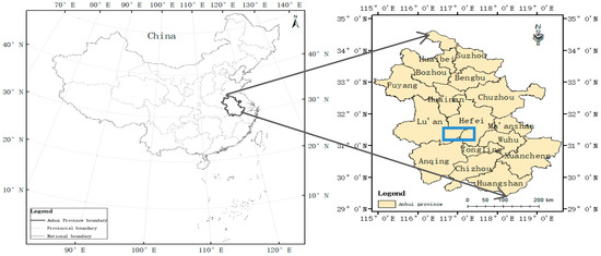
Figure 1.
Location of the study area.
The occurrence of FHB is completely natural in experimental fields in the winter wheat growing season, and survey data for a total of 89 ears were obtained through the visual method. The disease severity for each ear was visually determined by an experienced plant pathologist according to Rules for Monitoring and Forecast of the Wheat Head Blight (Fusarium graminearum Schw./Gibberella zeae (Schw.) Petch), issued in 2011 (GB/T 15796-2011). At the time of the survey, threshing occurred first. Then, the ratio of the number of diseased kernels to the total number of kernels of the ears was used as the severity of the individual ear (Figure 2). The grading standards of wheat FHB occurrence severity are shown in Table 1. In order to reduce the difficulty of identifying the severity of the disease, the severity of FHB was further reclassified into three classes: healthy (<1/5), mild (1/5≤ the ratio of diseased kernels <1/2), and severe (the ratio of diseased kernels ≥1/2).
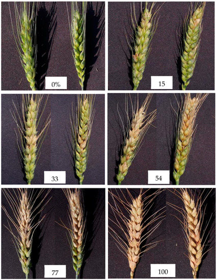
Figure 2.
FHB-infected ear of winter wheat at different stages of severity.

Table 1.
The grading standards of wheat Fusarium head blight (FHB) occurrence severity.
2.1.2. Spectral Measurement
An ASD (Analytical Spectral Devices) Field Spec Pro FR (Full range) (350–2500 nm) spectrometer was utilized to collect the spectral information of winter wheat ears. The spectral resolution of the spectrometer is 3 nm in the range of 350–1000 nm, 10 nm in the range of 1000–2500 nm, and the spectral sampling interval was 1 nm. Using a piece of 1 × 1 m black cloth with a hole in the middle, we pierced through the ear from under the holes, and placed the probe of the spectrometer on top of the ear to measure the erect spectrum. When measuring the spectrum of the front and side of the ear, we placed the front or side of the ear upward, bent the ear slightly, and fixed it on black cloth with double-sided tape or other means that did not affect the spectrum. The probe was also placed above the ear for spectral measurement. Each ear was measured 10 times at each angle, and the average value of the 10 measurements was recorded. Vertical measurement was performed using a conventional remote sensing method, but the information acquisition was incomplete. Horizontal measurements can reflect the disease infection more comprehensively. In order to better reflect the lesions caused by FHB in the spectral information to improve the identification accuracy of FHB, the spectrum measurement was carried out from three angles for each ear, namely, front, side, and erect (Figure 3). Spectra of all samples were collected between 10:00 and 14:00 (Beijing local time), under clear and cloudless breezy weather conditions. A calibration panel was used to calculate reflectance before each measurement.
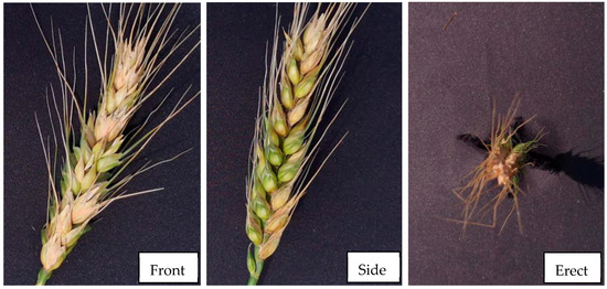
Figure 3.
FHB-infected ear of winter wheat at three measuring angles (front, side, and erect).
2.2. Data Preprocessing
Standardization of Spectral Data
The data of all samples in this experiment were collected at different times, growth periods, geographic areas, and for different wheat varieties. In order to eliminate spectral differences caused by the different backgrounds of data collection, the original data were standardized before analysis [22]. The spectra of all samples in area A were used as the standard spectra. The mean values of the spectra of the healthy samples in area A were divided by the mean values of the spectra of the healthy samples in areas B and C, respectively; thus, two ratio curves were obtained. The ratio curves reflect the spectral difference between the two areas [23]. The ratio at a certain wavelength was calculated using Equation (1):
where is the wavelength; represents the sum of reflectance of all healthy samples at wavelength in that area; is the reflectance; and A, B, and C are the spectra of samples in the areas of Guohe Town, Baihu Town, and Shucheng County, respectively.
The original spectrum of each sample acquired in area B and area C was multiplied by the corresponding ratio curve to obtain the standardized spectra. The standardized reflectance at a certain wavelength was calculated using Equation (2):
where is the reflectance of the original wavelength i of area B or area C; is the standardized reflectance.
The spectral standardization was used to improve the reliability of the results of spectral identification. In the process, the reflectance of the healthy samples in area A were used as the standard reflectance, and reflectance of the samples in areas B and C were adjusted to the same level of reflectance as the samples in area A. Therefore, the influence of the background difference of the three sets of data on the spectral discrimination were largely eliminated, and the relative difference between the spectra of the healthy samples and the diseased samples were not changed.
2.3. Analysis Methods
2.3.1. Selection of Candidate Spectral Features
Spectral derivative is a basic hyperspectral analysis technology. The transformation of the first-order derivative reflects the variation range of vegetation reflectance in each band, which can reduce the effects of atmospheric and background noise, and better reflect the essential features of plants [24]. Therefore, the spectral features sensitive to FHB were extracted by using the hyperspectral features of the first-order derivative transformation, including positional, area, ratio, and normalized index features (Table 2).
Table 2.
Hyperspectral features based on first order derivatives.
In FHB-infected ear tissues, absorption in the range of the chlorophyll bands rapidly decreased with development of infection as a result of destruction of chloroplasts, and successively, degradation of chlorophylls in cells attacked by fungi [16]. The dry shrinkage of ear tissue and the decrease of chlorophyll and water content causes the change of absorption position and spectral reflectivity of the red band [16,25]. The main purpose of continuum removal is to eliminate the irrelevant background information and enhance the spectrum absorption characteristic information [25]. The reflectance of the continuum removal in the range of 550–750 nm was calculated, and then the absorption characteristics were obtained. The main absorption characteristics are the absorption wavelength position, depth, width, and area (Table 3). The principle of continuum removal and the specific extraction process are described by Jing et al. [25] and Li et al. [26].
Table 3.
Spectral absorption features based on continuum removal.
The main purpose of this step was to find sensitive features of physiological and biochemical changes caused by FHB. The vegetation index method is a basic and commonly used information extraction technology in agricultural remote sensing monitoring research. Changes in plant pigment, moisture content, and internal structure occur when winter wheat is infected with pathogenic bacteria, and these changes can be reflected by spectral reflectance [17]. Based on prior knowledge, with reference to the application of various vegetation indices in the monitoring of plant diseases and insect pests, 16 vegetation indices based on hyperspectral data were selected and their applicability in assessing the severity of FHB was discussed. The indices and their groupings are as follows: indices used for the identification of pigment variation: Modified Chlorophyll Absorption Reflectance Index (MCARI), The Transformed Chlorophyll Absorption and Reflectance Index(TCARI), Chlorophyll Absorption Ratio Index (CARI), Triangular Vegetation Index (TVI), Anthocyanin Reflectance Index (ARI), Normalized Total Pigment to Chlorophyll Ratio Index (NPCI), Structure Insensitive Pigment Index (SIPI); for biophysical parameters: Normalized Difference Vegetation Index (NDVI), Green Normalized Difference Vegetation Index (GNDVI), Narrow-Band Normalized Difference Vegetation Index (NBNDVI), Modified Simple Ratio (MSR), Plant Senescence Reflectance Index (PSRI); for water and nitrogen content: Nitrogen Reflectance Index (NRI); for photosynthetic activity: Photochemical Reflectance Index (PRI), The Physiological Reflectance Index (PHRI); for greenness: Greenness Index (GI). The calculation formulas of the 16 vegetation indices are shown in Table 4.
Table 4.
Vegetation indices commonly used in stress studies.
2.3.2. Pre-Processing of the Spectral Feature Sets
In order to improve the accuracy of identification of the different stages of severity of FHB, and to ensure a high-efficiency operation, it is necessary to select the optimal spectral features from the candidate spectral features. The conditions of selection are as follows:
- (1).
- The spectral features are significantly correlated with the severity of FHB and the threshold determination coefficient is greater than 0.49 (R2 > 0.49).
- (2).
- For the three classes of samples (healthy, mild, and severe), the independent T-test was used to select spectral features that showed significant heterogeneity to each disease class (p < 0.001).
- (3).
- The spectral feature sets selected by the above two conditions were intersected to obtain an optimal spectral feature set sensitive to FHB and with significant heterogeneity between the three classes of disease severity.
- (4).
- The above steps were repeated from three angles—front, side, and erect—to obtain the optimal spectral feature set suitable for FHB identification.
2.3.3. Model Analysis
The spectral feature sets extracted by the above methods were used as an input variable to models and the models were constructed using the FLDA algorithm and the SVM algorithm, respectively. The FLDA algorithm reduces the dimensions of high-dimensional features, projects the data into a one-dimensional space, and finds an optimal projection direction that minimizes the within-class scatter and maximizes the between-class scatter [18]. The principle is as follows:
Suppose that a set in the original high-dimensional space contains samples , where samples belonging to the class are recorded as subset , ; samples belonging to the class are recorded as subset ; and samples belonging to the class are recorded as subset . In the original high-dimensional space, the pooled within-class scatter matrix is :
The between-class scatter matrix is :
In the one-dimensional space Y after projection, the pooled within-class scatter matrix is :
where is the mean vector of each class of samples in the original high-dimensional space; is the mean vector of each class of samples in the one-dimensional space Y after projection; is the mean vector of all of the samples.
The purpose is to find the best projection direction, so that the various samples of the one-dimensional space are separated as much as possible after projection. That is, the difference between the mean vector of each class of samples is as large as possible and the pooled within-class scatter matrix is as small as possible. The Fisher criterion function is defined as:
Let the denominator be equal to a non-zero constant, , and define the Lagrange function as:
where λ is the Lagrange multiplier.
The Fisher criterion function is used to obtain the partial derivative of ω. The partial derivative is set equal to zero to get the equation:
where is the maximum value, which is the best projection method.
In contrast, SVM is useful in dealing with linear indivisible cases. First, transform the input space into a high-dimensional space by nonlinear transformation (defining the suitable kernel function), and then find the optimal classification surface in the new space. Therefore, the nonlinear problem in the original space is transformed into a linear problem in the new space [19]. The principle is as follows:
The decision function of SVM in the original feature space is:
After the nonlinear transformation of the feature x, the new feature is recorded as , then the SVM decision function constructed in the new feature space is:
When observing Equations (9) and (10), it is found that the inner product in the original space becomes in the new space after the transformation. Because the inner product in the new feature space is also a function of the original feature, it is recorded as a kernel function:
Thus, Equation (10) can be rewritten as:
where is the optimal solution to the optimization problem.
It is found that a nonlinear SVM can be constructed by selecting a suitable kernel function. Previous studies have shown that the radical basis function (RBF) is better than the polynomial kernel function and sigmoid tanh [41], so the RBF was used to construct a nonlinear SVM in this research.
In order to further improve the accuracy of the model, the LDA–SVM model was constructed, combining the advantages of the FLDA and SVM. The original high-dimensional features were reduced by the FLDA algorithm, and the low-dimensional eigenvectors obtained were used as input variables of the SVM model. Figure 4 summarizes the basic steps from hyperspectral signatures to three different models, and then to final identification.
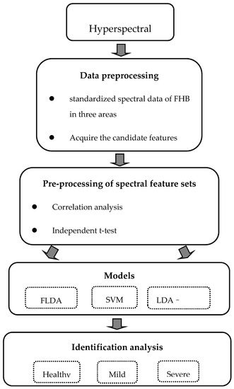
Figure 4.
General workflow for identification of wheat Fusarium head blight; FLDA (fisher’s linear discriminant analysis); SVM (support vector machine); LDA–SVM (the combination of FLDA and SVM).
3. Results and Discussion
3.1. Evaluation of the Ability of Various Features to Identify Fusarium Head Blight
3.1.1. The Features of First-Order Derivatives
Compared to the original spectrum, it is found that the correlation between the first-order derivative spectrum and the severity of FHB is significantly improved, and the correlation coefficient is up to 0.8 (Figure 5).
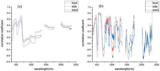
Figure 5.
Correlation coefficient curves of different spectra and severity of disease. (a) The original spectrum. (b) First order derivative spectrum.
Table 5 shows that six spectral features of first-order derivative for the front and side samples, namely, SDy, SDy/SDb, SDg/SDb, (SDr − SDy)/(SDr + SDy), (SDy − SDb)/(SDy + SDb), and (SDg − SDb)/(SDg + SDb), are significantly correlated (p-value < 0.001) with disease severity and the absolute values of correlation coefficients are greater than 0.7 (|R| > 0.7). Four spectral features for erect samples, namely, SDy, SDg/SDb, (SDr − SDy)/(SDr + SDy), and (SDg − SDb)/(SDg + SDb), are significantly correlated (p-value < 0.001) with severity and the absolute values of correlation coefficients are greater than 0.7 (|R| > 0.7).
Table 5.
Correlation between derivative features and disease severity.
3.1.2. The Features of Continuum Removal
Table 6 shows the spectral features of band depth H and absorption area A, which are highly negatively correlated with the severity of disease of the ear at three angles. The absolute values of the correlation coefficients between the spectral features (H and Area) and disease severity for the front and side samples were higher than 0.7 (|R| > 0.7). The absolute values of the correlation coefficient for the erect samples were slightly lower than 0.7 and showed a very significant correlation (p-value < 0.001). The band characteristic position and the band widths w1 and w2 have no significant correlation with the severity of Fusarium head blight.
Table 6.
Correlation between continuum removal features and disease severity.
3.1.3. Vegetation Indices
Information about infected wheat was extracted via commonly used vegetation indices in this research. The vegetation indices are strongly correlated with the severity of the disease (p-value < 0.001) and the absolute values of correlation coefficients are greater than 0.7 (|R| > 0.7), as shown in Table 7. The sensitive vegetation indices for front samples are NDVI, NBNDVI, NRI, PSRI, SIPI, NPCI, MSR, and GI; for side samples are NDVI, NBNDVI, NRI, PSRI, SIPI, NPCI, and MSR; and for erect samples are NDVI, NBNDVI, PSRI, SIPI, and MSR.
Table 7.
Correlation between vegetation indices and disease severity.
3.2. Selection of Spectral Feature Sets
According to the selection conditions, the number of selected features was 16, 15, and 9 for the three angles (Table 8), and these features were used as the input variables for models. From the order of accuracy in Table 8, it can be found that the ability of the first-order derivative features to identify FHB are better than the continuum removal features and vegetation indices. The features of continuum removal are not sensitive to FHB for erect samples. The sensitive features for the front samples were almost the same as the side samples, and the number of sensitive features for the erect samples was the least. The number of sensitive features for erect samples was not only the least, but also the ability of single features to identify FHB was much lower than the ability of the front and side samples. Because the disease occurrence of the middle and bottom kernels of the ear was ignored when the erect ear was measured, the correlation between the actual disease severity and the spectral features was not significant.
Table 8.
Selected spectral feature variables.
3.3. Identification of Diseased Samples with Different Degrees of Severity
A total of 89 samples were collected at three angles in this experiment, of which 54 random samples were used as training samples to construct models and 35 samples were used as test samples for model validation. According to the correlation analysis and the independent sample T-test method, the spectral features sensitive to different disease severity were used as input variables. The FLDA, SVM, and LDA–SVM models were used to construct the identification model. The confusion matrix for classification based on the validation samples and the various accuracy evaluation indicators are shown in Table 9.
Table 9.
Confusion matrix and classification accuracies.
For the front samples, the overall accuracies of the disease severity based on the FLDA, SVM, and LDA–SVM models are 77.1%, 80.0% and 85.7%, respectively, and the Kappa coefficients are 0.639, 0.683, and 0.770, respectively. For the side samples, the overall accuracies based on the three models are 85.7%, 82.9%, and 88.6%, respectively, and the Kappa coefficients are 0.762, 0.728, and 0.808, respectively. For the erect samples, the overall accuracies of the disease based on the three models are 62.9%, 65.7%, and 68.6%, respectively, and the Kappa coefficients are 0.416, 0.424, and 0.506, respectively. The accuracy and Kappa coefficient comparison for the three models are summarized in Figure 6.
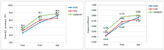
Figure 6.
Comparison curve of model accuracy and kappa coefficient.
From the above results, the identification of disease severity for the front and side samples based on three modes are generally ideal and the LDA–SVM model has the best identification effect, with accuracies of 85.7% and 88.6% and Kappa coefficients of 0.770 and 0.808, respectively. However, the classification accuracy for erect samples was slightly lower, at 68.6%. Overall, the accuracy of the SVM model is better than the FLDA model, but the effect is not obvious. Perhaps the combination of the two parameters of the kernel function coefficient and the penalty coefficient of the SVM is not optimal. The parameters are selected using manual methods, which are not only inefficient with low classification accuracy, but also prone to overfitting [42]. There are a lot of feature variables and excessive variables that not only increase the difficulty of calculation, but also make the interpretability of the model worse. Therefore, combining the advantages of the FLDA and SVM algorithms, the FLDA is used to reduce the dimension of the original feature variables, and the resulting low-dimensional eigenvectors are used as the input variables of the SVM model, effectively improving the accuracy of the model. In addition, from the perspective of user’s accuracy and producer’s accuracy, the accuracy of the LDA–SVM model reach more than 80% or even 100% for the front and side angles, which is obviously better than the FLDA model or SVM model. The producer’s accuracy values of healthy samples are 92.3%, 81.8%, and 81.8% for the front, side, and erect angles, respectively. This indicates that the LDA–SVM model can ideally identify discoloration or maturation from FHB-infected ears.
The classification accuracy for side samples is higher than the front, and for the erect samples is the lowest. Therefore, we can conclude that the side is the best angle to detect FHB, followed by the front. The reason for that is the fact that the classification accuracy of ears infected with FHB is affected by the measurement angle of the ear. The result is related to the number of input features of the identification model and the ability of the features to identify the FHB. The number of sensitive spectral features obtained for the side samples is more than the front, whereas the number of sensitive features for erect samples is only half that of the front and side samples. The sensitive spectral features for the side samples are superior to the front, and the front samples are superior to the erect samples with respect to the ability to identify FHB.
In order to evaluate the contribution of each selected feature to the classification in the model, the weights were calculated using the relief algorithm (Figure 7) [43]. The results show that the features, including (SDg − SDb)/(SDg + SDb), SDg/SDb, NRI, SDb, SIPI and PSRI, have important weights at the side angle; the features of SDg/SDb, (SDg − SDb)/(SDg + SDb), (SDr − SDy)/(SDr + SDy), SIPI, and NRI have important weights at the front angle; the features of SDg/SDb and (SDg − SDb)/(SDg + SDb) have important weights at the erect angle. Among them, the first-order derivative features of SDg/SDb and (SDg − SDb)/(SDg + SDb) are most dominant in the model produced for the three angles, and they have huge potential for FHB identification. The result is consistent with the previous finding that the ability of the first-order derivative features to identify FHB is better than for the continuum removal features and vegetation indices.
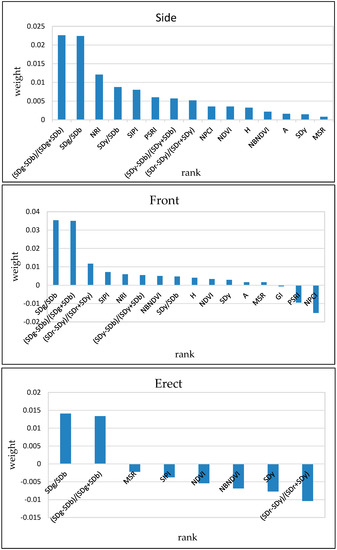
Figure 7.
The important weights of selected features in the models at side, front, and erect angles.
4. Conclusions
The effects of background differences of data collection in the three areas were eliminated by standardizing the spectral data prior to analysis. Correlation analysis and independent sample T-tests were used to verify the feasibility of identifying the disease severity by using the spectral feature sets, which were extracted by the combination of derivative features, continuum removal features, and common vegetation indices at the ear level. The FLDA and SVM models are constructed by using the sensitive spectral feature sets as input variables, and the results show that the accuracy of the two models are ideal, although the overall accuracy of the SVM was slightly better than the FLDA, but the effect is not obvious. The LDA–SVM model combined the advantages of FLDA and SVM, and had a better identification accuracy than the FLDA or SVM models. The identification accuracy for the three angles is 88.6%, 85.7%, and 68.6%, respectively. The results show that: (1) the selected spectral features have great potential in detecting ears infected with FHB, especially the first-order derivative features SDg/SDb and (SDg − SDb)/(SDg + SDb); (2) the LDA–SVM model has a good effect on identifying the severity of FHB in a complex, farmland environment; and (3) of the three angles used in the experiment, the side was the best angle for detecting FHB, followed by the front. However, the identification effect for the erect samples is poor (68.6%), which needs to be improved. The results are of great significance for identifying diseases of different severity at ear level, and provide a theoretical reference for the further study of identification of FHB at the canopy scale or regional scale.
Traditionally, the methods of disease assessment have been visually investigated in the field by experienced farmers or pathologists. Visual rating is unavoidably subjective, and the error range largely depends on the personnel skills of the evaluator. The emergence of hyperspectral measurements has distinct advantages over conventional visual inspection, allowing the information to be collected repeatedly, automatically, and objectively. In this study, a convenient, simple, and effective method was used to establish a model that can accurately identify the disease severity of wheat at the filling and maturity stages, reducing the time and effort related to manual investigation. Furthermore, it is easy to implement. The method can be used to identify FHB-infected wheat at the mild disease stage and guide field management accurately. For example, in the case of FHB infections in wheat, it can identify the area of infection and prevent infections in neighboring areas. This information can help farmers to segregate the harvesting of severely affected areas of fields to avoid toxins entering the food chain. In addition, the model can be used to collect FHB data, and can provide data support and validation for some research studies.
Author Contributions
All authors contributed to the conceptualization. Z.W. performed the formal analysis and original draft writing. L.H. and W.H. contributed to the supervision. H.M. and J.Z. performed the writing, review, and editing. All authors contributed to the paper.
Funding
This research was funded by Anhui Provincial Science and Technology Project (16030701091), the science and technology service program of the Chinese Academy of Sciences (KFJ-STS-ZDTP-054), Hainan Provincial Key R&D Program of China, and Natural Science Research Project of Anhui Provincial Education Department (KJ2019A0030).
Acknowledgments
The authors are grateful to Linyi Liu for valuable technical guidance. The authors would also like to thank Chao Ruan and Jing Jiang for their help with data collection.
Conflicts of Interest
The authors declare no conflict of interest.
Abbreviations
The following abbreviations are used in this manuscript:
| PRI | Photochemical Reflectance Index |
| PHRI | The Physiological Reflectance Index |
| MCARI | Modified Chlorophyll Absorption Reflectance Index |
| TVI | Triangular Vegetation Index |
| ARI | Anthocyanin Reflectance Index |
| NDVI | Normalized Difference Vegetation Index |
| GNDVI | Green Normalized Difference Vegetation Index |
| NBNDVI | Narrow-Band Normalized Difference Vegetation Index |
| NRI | Nitrogen Reflectance Index |
| PSRI | Plant Senescence Reflectance Index |
| SIPI | Structure Insensitive Pigment Index |
| NPCI | Normalized Total Pigment to Chlorophyll Ratio Index |
| TCARI | The Transformed Chlorophyll Absorption and Reflectance Index |
| CARI | Chlorophyll Absorption Ratio Index |
| GI | Greenness Index |
| MSR | Modified Simple Ratio |
References
- Song, Y.; Linderholm, H.W.; Wang, C.; Tian, J.; Huo, Z.; Gao, P.; Song, Y.; Guo, A. The influence of excess precipitation on winter wheat under climate change in China from 1961 to 2017. Sci. Total Environ. 2019, 690, 189–196. [Google Scholar] [CrossRef]
- Zhang, J.; Yi, Y.; Wang, J.; Chen, S.; Li, G. Research progress of control techniques on wheat scab. China Plant. Prot. 2014, 34, 24–28, 53. [Google Scholar]
- McMullen, M.; Jones, R.; Gallenberg, D. Scab of Wheat and Barley: A Re-emerging Disease of Devastating Impact. Plant. Dis. 1997, 81, 1340–1348. [Google Scholar] [CrossRef] [PubMed]
- Bennett, J.W.; Klich, M. Mycotoxins. Clin. Microbiol. Rev. 2003, 16, 497–516. [Google Scholar] [CrossRef] [PubMed]
- Goswami, R.S.; Kistler, H.C. Heading for disaster: Fusarium graminearum on cereal crops. Mol. Plant. Pathol. 2004, 5, 515–525. [Google Scholar] [CrossRef]
- Ropelewska, E.; Zapotoczny, P. Classification of Fusarium-infected and healthy wheat kernels based on features from hyperspectral images and flatbed scanner images: A comparative analysis. Eur. Food Res. Technol. 2018, 244, 1453–1462. [Google Scholar] [CrossRef]
- Hu, X.; Rocheleau, H.; McCartney, C.; Biselli, C.; Bagnaresi, P.; Balcerzak, M.; Fedak, G.; Yan, Z.; Valè, G.; Khanizadeh, S.; et al. Identification and mapping of expressed genes associated with the 2DL QTL for fusarium head blight resistance in the wheat line Wuhan 1. BMC Genet. 2019, 20, 47. [Google Scholar] [CrossRef]
- Karlsson, I.; Friberg, H.; Kolseth, A.K.; Steinberg, C.; Persson, P. Agricultural factors affecting Fusarium communities in wheat kernels. Int. J. Food Microbiol. 2017, 252, 53–60. [Google Scholar] [CrossRef]
- Steiner, B.; Buerstmayr, M.; Michel, S.; Schweiger, W.; Lemmens, M.; Buerstmayr, H. Breeding strategies and advances in line selection for Fusarium head blight resistance in wheat. Trop. Plant. Pathol. 2017, 42, 165–174. [Google Scholar] [CrossRef]
- Sip, V.; Chrpova, J.; Sterbova, L.; Palicová, J. Combining ability analysis of fusarium head blight resistance in European winter wheat varieties. Cereal Res. Commun. 2017, 45, 260–271. [Google Scholar] [CrossRef][Green Version]
- Xu, Y.; Hideki, N. The infection process of wheat scab pathogen. J. Nanjing Agric. Univ. 1989, 12, 33–38. [Google Scholar]
- Hernandez Nopsa, J.F.; Daglish, G.J.; Hagstrum, D.W.; Leslie, J.F.; Phillips, T.W.; Scoglio, C.; Thomas-Sharma, S.; Walter, G.H.; Garrett, K.A. Ecological networks in stored grain: Key postharvest nodes for emerging pests, pathogens, and mycotoxins. Bioscience 2015, 65, 985–1002. [Google Scholar] [CrossRef]
- Liang, K.; Du, Y.Y.; Lu, W.; Wang, G.; Xu, J.H.; Shen, M.X. Identification of Fusarium Head Blight Wheat Based on Hyperspectral Imaging Technology. Trans. Chin. Soc. Agric. Mach. 2016, 47, 309–315. [Google Scholar] [CrossRef]
- Delwiche, S.R.; Rodriguez, I.T.; Rausch, S.R.; Graybosch, R.A. Estimating percentages of fusarium-damaged kernels in hard wheat by near-infrared hyperspectral imaging. J. Cereal Sci. 2019, 87, 18–24. [Google Scholar] [CrossRef]
- Whetton, R.L.; Waine, T.W.; Mouazen, A.M. Hyperspectral measurements of yellow rust and fusarium head blight in cereal crops: Part 2: On-line field measurement. Biosyst. Eng. 2018, 167, 144–158. [Google Scholar] [CrossRef]
- Bauriegel, E.; Giebel, A.; Geyer, M.; Schmidt, U.; Herppich, W.B. Early detection of Fusarium infection in wheat using hyper-spectral imaging. Comput. Electron. Agric. 2011, 75, 304–312. [Google Scholar] [CrossRef]
- Jin, X.; Jie, L.; Wang, S.; Qi, H.; Li, S. Classifying Wheat Hyperspectral Pixels of Healthy Heads and Fusarium Head Blight Disease Using a Deep Neural Network in the Wild Field. Remote Sens. 2018, 10, 395. [Google Scholar] [CrossRef]
- Huang, W.; Zhang, J.; Luo, J.; Zhao, J.; Huang, L.; Zhou, X. Remote Sensing Monitoring and Forecasting of Crop. Diseases and Insect Pests, 1st ed.; Beijing Science Press: Beijing, China, 2015. [Google Scholar]
- Zhang, X. Pattern Recognition, 3rd ed.; Tsinghua University Press: Beijing, China, 2010. [Google Scholar]
- Huang, L.; Liu, W.; Huang, W.; Zhao, J.; Song, F. Remote sensing monitoring of winter wheat powdery mildew based on wavelet analysis and support vector. Trans. Chin. Soc. Agric. Eng. 2017, 33, 188–195. [Google Scholar] [CrossRef]
- Zhao, J.; Xu, C.; Xu, J.; Huang, L.; Zhang, D.; Liang, D. Forecasting the wheat powdery mildew (Blumeria graminis f. Sp. tritici) using a remote sensing-based decision-tree classification at a provincial scale. Australas. Plant. Pathol. 2018, 47, 53–61. [Google Scholar] [CrossRef]
- Zhang, J.; Pu, R.; Huang, W.; Yuan, L.; Luo, J.; Wang, J. Using in-situ hyperspectral data for detecting and discriminating yellow rust disease from nutrient stresses. Field Crop. Res. 2012, 134, 165–174. [Google Scholar] [CrossRef]
- Yuan, L.; Bao, Z.; Tian, J.; Xing, C.; Zhang, H. Spectral Differentiation among Different Diseases and Pests in Winter Wheat Using Continuous Wavelet Analysis. Geogr. Geo-Inf. Sci. 2017, 33, 28–34. [Google Scholar] [CrossRef]
- Jia, W.Y.; Zhi, Q.C.; Jin, S.Z.; He, S.W.; Yue, L.J.; Shu, Y.Y. An Approach to Distinguishing Between Species of Trees and Crops Based on Hyperspectral Information. Spectrosc. Spectr. Anal. 2018, 38, 3890–3896. [Google Scholar] [CrossRef]
- Jing, X.; Wang, J.; Song, X.; Xu, X.; Chen, B.; Huang, W. Continuum removal method for cotton verticillium wilt severity monitoring with hyperspectral data. Trans. CSAE 2010, 26, 193–198. [Google Scholar] [CrossRef]
- Li, F.L.; Chang, Q.R. Estimation of Winter Wheat Leaf Nitrogen Content Based on Continuum Removed Spectra. Trans. Chin. Soc. Agric. Mach. 2017, 48, 174–179. [Google Scholar] [CrossRef]
- Gamon, J.A.; Serrano, L.; Surfus, J.S. The Photochemical Reflectance Index: An optical indicator of photosynthetic radiation use efficiency across species, functional types and nutrient levels. Oecologia 1997, 112, 492–501. [Google Scholar] [CrossRef]
- Daughtry, C.S.T.; Walthall, C.L.; Kim, M.S.; De Colstoun, E.B.; McMurtrey Iii, J.E. Estimating corn leaf chlorophyll concentration from leaf and canopy reflectance. Remote Sens. Environ. 2000, 74, 229–239. [Google Scholar] [CrossRef]
- Broge, N.H.; Mortensen, J.V. Deriving green crop area index and canopy chlorophyll density of winter wheat from spectral reflectance data. Remote Sens. Environ. 2002, 81, 45–57. [Google Scholar] [CrossRef]
- Gitelson, A.A.; Merzlyak, M.N.; Chivkunova, O.B. Optical properties and nondestructive estimation of anthocyanin content in plant leaves. J. Photochem. Photobiol. 2001, 74, 38–45. [Google Scholar] [CrossRef]
- Rouse, J., Jr.; Haas, R.H.; Schell, J.A.; Deering, D.W. Monitoring vegetation systems in the great plains with ERTS. In Proceedings of the Third ERTS Symposium, College Station, TX, USA, 10–14 December 1973; Volume 1, pp. 309–317. [Google Scholar]
- Thenkabail, P.S.; Smith, R.B.; Pauw, E.D. Hyperspectral vegetation indices and their relationships with agricultural crop characteristics. Remote Sens. Environ. 2000, 71, 158–182. [Google Scholar] [CrossRef]
- Filella, I.; Serrano, L.; Serra, J.; Penuelas, J. Evaluating wheat nitrogen status with canopyreflectance indices and discriminant analysis. Crop. Sci. 1995, 35, 1400–1405. [Google Scholar] [CrossRef]
- Merzlyak, M.N.; Gitelson, A.A.; Chivkunova, O.B.; Rakitin, V.Y. Non-destructive optical detection of leaf senescence and fruit ripening. Physiol. Plant. 1999, 106, 135–141. [Google Scholar] [CrossRef]
- Peñuelas, J.; Inoue, Y. Reflectance indices indicative of changes in water and pigment contents of peanut and wheat leaves. Photosynthetica 1999, 36, 355–360. [Google Scholar] [CrossRef]
- Peñuelas, J.; Gamon, J.A.; Fredeen, A.L.; Merino, J.; Field, C.B. Reflectance indices associated with physiological changes in intro-gen and water-limited sunflower leaves. Remote Sens. Environ. 1994, 48, 136–146. [Google Scholar] [CrossRef]
- Haboudane, D.; Miller, J.R.; Tremblay, N.; Zarco-Tejada, P.J.; Dextraze, L. Integrated narrow-band vegetation indices for predicting of crop chlorophyll content for application to precision agriculture. Remote Sens. Environ. 2002, 81, 416–426. [Google Scholar] [CrossRef]
- Kim, M.S.; Daughtry, C.S.T.; Chappelle, E.W.; McMurtrey, J.E.; Walthall, C.L. The use of high spectral resolution bands for estimating absorbed photosynthetically active radiation (APAR). In Proceedings of the 6th International Symposium on Physical Measurements and Signatures in Remote Sensing, Greenbelt, MD, USA, 1 January 1994; pp. 299–306. [Google Scholar]
- Zarco-Tejada, P.J.; Berjón, A.; López-Lozano, R.; Miller, J.R.; Martín, P.; Cachorro, V.; González, M.R.; De Frutos, A. Assessing vineyard condition with hyperspectral indices: Leaf and canopy reflectance simulation in a row-structured discontinuous canopy. Remote Sens. Environ. 2005, 99, 271–287. [Google Scholar] [CrossRef]
- Haboudane, D.; Miller, J.R.; Pattey, E.; Zarco-Tejada, P.J.; Strachan, I.B. Hyperspectral vegetation indices and novel algorithms for predicting green LAI of crop canopies: Modeling and validation in the context of precision agriculture. Remote Sens. Environ. 2004, 90, 337–352. [Google Scholar] [CrossRef]
- Feng, G. Parameter optimizing for Support Vector Machines classification. Comput. Eng. Appl. 2011, 47, 123–124. [Google Scholar] [CrossRef]
- Zhou, Q.C.; Liu, J.; Liu, L.; Huang, D.; Deng, L.; Jiang, Q. Research on fault fiagnosis penalty coefficient and kernel function coefficient optimization of ventilation system based on SVM. J. Saf. Sci. Technol. 2019, 15, 45–51. [Google Scholar] [CrossRef]
- Huang, L.L.; Tang, J.; Sun, D.D.; Luo, B. Feature selection algorithm based on multi-label ReliefF. J. Comput. Appl. 2018, 10, 2888–2890, 2898. [Google Scholar] [CrossRef]
© 2019 by the authors. Licensee MDPI, Basel, Switzerland. This article is an open access article distributed under the terms and conditions of the Creative Commons Attribution (CC BY) license (http://creativecommons.org/licenses/by/4.0/).