A New Method for Positional Accuracy Control for Non-Normal Errors Applied to Airborne Laser Scanner Data

Abstract

A new statistical method for the quality control of the positional accuracy, useful in a wide range of data sets, is proposed and its use is illustrated through its application to airborne laser scanner (ALS) data. The quality control method is based on the use of a multinomial distribution that categorizes cases of errors according to metric tolerances. The use of the multinomial distribution is a very novel and powerful approach to the problem of evaluating positional accuracy, since it allows for eliminating the need for a parametric model for positional errors. Three different study cases based on ALS data (infrastructure, urban, and natural cases) that contain non-normal errors were used. Three positional accuracy controls with different tolerances were developed. In two of the control cases, the tolerances were defined by a Gaussian model, and in the third control case, the tolerances were defined from the quantiles of the observed error distribution. The analysis of the test results based on the type I and type II errors show that the method is able to control the positional accuracy of freely distributed data.

1. Introduction

Digital topographic data are indispensable for modern modelling needs in many science branches (e.g., environmental planning, forestry, geology, hydrology, climate change, etc.). Airborne Laser Scanner (ALS) systems record terrain elevation, terrain structure lines, buildings, vegetation and, in general, any feature present in the field and that can be detected by its resolution. One type of product of great importance that is derived from ALS are digital terrain models (DTM). DTM generation using only LiDAR data present limitation to simultaneously distinguish complicated terrain situations (e.g., discontinuities and shape ridges), highly fragmented landscapes, and a variety of objects ([1]). The vertical accuracy of LiDAR-derived DTM for uncovered and vegetated areas is assessed in [2]. By means of 193 check-points measured with GNSS-RTK, the mean vertical accuracy reached 0.091 m, while the RMSE was 0.115 m. Related to volume changing (DEM comparison), in [3], the vertical difference of ALS data for vegetated and no vegetated area of a landslide is reported 0.3 and 0.125 m respectively. In the case of the errors caused by the forest vegetation structure, the presence of leaf-on vegetation causes significant errors (RMSE > 1 m), in contrast with the leaf-off conditions (RMSE = 0.22 m) according to the results presented by [4]. In [5], the influence of factors such as forest structure, slope, off-nadir angle, understory vegetation and filtration and interpolation algorithm on ALS-derived DTM accuracy in mixed mountainous forests was evaluated. The RMSE and the mean error ranged from 0.19 to 0.23 m, and from 0.13 to 0.16 m, respectively, being the slope and the undergrowth vegetation the most important factors influencing DTM accuracy. In [6], as part of a multitemporal study of an alpine rock glacier, the signed discrepancy for stable areas yielded a standard deviation of 0.23 m for a time span of 5 years. LiDAR precision is also evaluated for physical features, as for example in [7], where the LiDAR error for dimensional features of a bridge and several fence posts reach up to 23.5%.

The best way to assess or control positional accuracy is by applying standardized methods. Some of them are the National Standard for Spatial Data Accuracy [8], the Engineering Map Accuracy Standard [9], the Standardization Agreement 2215 [10], the Positional Accuracy Standards for Digital Geospatial Data [11] and the European Spatial Data Research (EuroSDR) through its proposal of accuracy measures for digital surface models based on parametric approaches [12]. More precisely, EuroSDR proposes the use of the relative vertical accuracy, the absolute vertical accuracy, and the relation pointed out between them. Ariza-López and Atkinson-Gordo [13] presented an analysis of the main features of some of these methods, and in many cases, they are based on the assumption of the normality of the errors. However, many authors [14,15,16,17,18,19] indicate that positional errors are not normally distributed.

The normal distribution is a suitable distribution for representing real-valued random variables. Therefore, the situation described above regarding positional errors leads to three important questions: (1) why may error data be non-normally distributed? (2) how does non-normality affect the methods based on the assumption of normally distributed data? and finally, (3) how can we work with non-normal data?

For the first question, and from a general point of view, six main causes of the non-normality of errors can be considered: (i) the presence of too many extreme values (i.e., outliers), (ii) the overlap of two or more processes, (iii) insufficient data discrimination (e.g., round-off errors, poor resolution), (iv) the elimination of data from the sample, (v) the distribution of values close to zero or the natural limit, and (vi) data following a different distribution (e.g., Weibull, Gamma, etc.). Additionally, some of these causes can appear together.

With regards to the second question and working with methods based on the normality assumption, the non-normality of the data can have various consequences depending on the degree of non-normality of the data and the robustness of the method applied. In this case, the non-normality violates a basic assumption of the method, and this violation is important from a strict perspective. For instance, the minimum quadratic estimators are not efficient, and the confidence intervals and hypothesis tests of parameters can only be approximated. Although it is possible that the results of a method can be considered valid if the non-normality is slight, the results may be completely incorrect if the non-normality is significant [20]. As an example of the above, if the error data contain a few outliers, their elimination from the analysis to achieve normality can give an acceptable result, but if the number of outliers is very large, this elimination is no longer possible.

Finally, to answer the third question, it is necessary to consider two very different situations: (a) data are not normally distributed but are distributed following another parametric distribution function (e.g., Weibull, Gamma, etc.), (b) data do not follow a distribution. In both cases, methods based on normal data are inadequate, but if a parametric distribution can be applied, the properties and parameters of such a distribution can help us work with these data. If the data are freely distributed, an observed distribution function is required for the analysis. Working with observed distributions is more complicated than working with parametric models, but this circumstance does not prevent estimation and decision-making (quality control) within a probabilistic framework [21].

Positional accuracy assessment methods based on free-distributed data are scarce. Following the analysis of Ariza-López & Rodríguez-Avi [22], the National Map Accuracy Standard [23] can be considered a method with capabilities to work with free-distributed data. In addition, it is possible to use percentiles when working with this type of error data, but the proposals for the use of percentiles, such as that of Maune [14], are merely descriptive, in the statistical sense, and no method for quality control is given. Error counting is the statistical technique that is used to cope with these cases. Following this idea, several methods exist: Cheok et al. [24] describe a method that allows the control of building plans; Ariza-López & Rodríguez-Avi [25] propose a method for positional accuracy control of line strings; the Spanish standard for positional accuracy control [26] proposes the use of the defect counting method established by the International Standard ISO 2859 [27]. All of these methods are able to work with free-distributed error data but are very limited by the statistical model that is applied (i.e., the binomial distribution function).

The objective of this paper is to propose a new and general statistical method for positional accuracy control that can be applied to any kind of data without the need for any underlying statistical hypothesis, e.g., ALS error data, and in general, for any free-distributed error data or non-normally distributed data. The motivation of this work is twofold: to have a method of quality control that is not subject to the need for normal positional errors and, on the other hand, the possibility of controlling the observed error distribution as much as desired.

2. Materials and Methods

This section includes a detailed presentation of the datasets used as examples and the new method based on the application of the multinomial law. The data presentation covers the original data capture methods, the error calculation procedure, and the error characterization. The presentation of the new method covers three more important issues: the conceptual model, tolerance assignment and p-value calculation.

2.1. Materials

The original dataset corresponds to an ALS flight campaign executed over the city of Avila (Spain). The data were acquired in April 2012 with a Leica ALS50-II sensor with a flying height of 1000 m, resulting in an original ground spacing of approximately 2 points/m² over urban and open terrain areas. Different test bed sites in terms of roughness and slope were used to validate the accuracy assessment of the ALS: an urban road stretch covered with asphalt (denoted by infrastructure), a building with variable heights (denoted by urban) and an abrupt natural area with vegetation, slopes and rocks (denoted by natural), (Figure 1a) as well as some point cloud image from ALS (Figure 1b).

Reference data were derived [28] by a mobile mapping system (MMS), Optech Lynx, in May 2012, so that no significant changes of the test sites were possible. Although static laser scanning techniques usually provide better quality than MMS, especially if only a single station is required, everything become more complicated when we address large urban, infrastructure and natural areas since static laser technologies require many stations and thus error propagation and processing steps would make these static technologies less efficient.

Table 1. Main characteristics of the three test bed sites.

	Infrastructure	Urban	Natural
Area (m2)	408.5	180.8	1772.3
Mean density (points/m2)	1.03	3.56	2.23
Max height difference (m)	1.57	1.65	14.64
90th percentile Roughness (m)	0.013	0.138	0.107

presents information characterizing the three areas used (surface, density of LiDAR points, roughness and maximum height difference). More technical specifications about the ALS and MMS equipment are outlined in

Table 2. Technical characteristics of the LIDAR system.

Sensor	ALS50_II SN48
X,Y position precision	0.320 m
Z position precision	0.120 m
Laser pulse rate used	95.8 KHz
Scan field of view (half angle)	22.50°
Point density (average)	1.87 m2
Number of returns	4
Laser divergence	0.22 mr
Max field of view	75°
Max rate of acquisition	120 KHz
Wavelength	1064 nm
Standard deviation of GNSS	0.05 m

and

Table 3. Technical characteristics of the mobile mapping system (MMS) Optech Lynx.

Sensor	Optech Lynx
X,Y position precision	0.030 m
Z position precision	0.050 m
Roll and Pitch	0.005°
True heading	0.015°
Measuring principle	Time of Flight (ToF)
Maximum range	200 m
Range precision	8 mm, (1σ)
Range accuracy	±10 mm, (1σ)
Laser measurement rate	75–500 kHz
Measurement per laser pulse	Up to 4 simultaneous
Scan frequency	80–200 Hz
Laser wavelength	1550 nm (near-infrared)
Scanner field of view	360°
Operating temperature	10 °C–40 °C
Angular resolution	0.001°

.

Regarding Table 2, there are some components that contribute to the final horizontal (X,Y) and vertical (Z) precision in the actual ALS dataset: (i) errors due to calibration of the GNSS/IMU and the scanner assembly; (ii) errors due to the complexity of the object (i.e., sloping terrains can lead to larger errors in the horizontal and vertical components); (iii) errors due to multipath reflections produced when the laser beam is reflected by another object on the ground before reaching the detector.

Regarding planimetric error, it should be noted that the Y coordinate will be mainly affected by the roll angle, whereas the X coordinate will be affected by the pitch angle. Laser parameters (scan angle and range) will directly affect the Y coordinate.

The positional accuracy samples of the three study cases (infrastructure, urban and natural) were computed using the open source software CloudCompare [29]. For the three positional accuracy samples, the MMS data were used as the ground truth. In the infrastructure case, the positional accuracy between the MMS and ALS points was computed as Z discrepancies (1D) due to its planar nature. In the other two study cases (urban and natural), the error was computed using the 3D coordinates (3D) since the normal vector of the surfaces does not follow the Z axis. For a point cloud to point cloud comparison, if the reference cloud is dense enough, the distance to its nearest neighbor is almost as precise as the true distance on the real-world surface. However, the resulting distance is the vector’s module, namely, the unsigned distance. To provide signed errors, a local 2.5D triangulation was created from the MMS point cloud (of higher point density), which defines the normal vectors according to each triangular face. Moreover, meshing is also carried out since the distance computation could fail in poor/irregular density clouds. The distance from each point in the ALS cloud is computed to the nearest triangle in the reference mesh (MMS) along its normal vector. This procedure is generally more robust, faster and more accurate than a nearest neighbor procedure, but it is constrained according to the mesh quality.

The results of

Table 4. Results of gaussian assessment and normality test for the test sites.

	Infrastructure	Urban	Natural
Sample size n	575	863	4432
Kurtosis	114.9	−0.6	3.3
Skewness	8.4	−0.3	−1.3
Sample mean µ	−0.022 m	−0.071 m	−0.018 m
Standard deviation σ	±0.034 m	±0.083 m	±0.077 m
Robust Jarque Bera
Statistic	3.5·106	21.8	4502.8
Critical Value	5.99	5.99	5.99
p-value	<1·10−6	3.5·10−5	<1·10−6
Result	Normality rejected	Normality rejected	Normality rejected

and Figure 2 characterize the error data and verify that the error data in the three study cases are non-normal. The check of the normality assumption can be performed by the application of numerical tests or by visual methods (e.g., quantile-quantile plots—Figure 2), in cases where the sample size is very large. In this study, since the sample sizes are less than 5000 points, the robust version [30] of the Jarque-Bera test of normality was employed. The original Jarque-Bera test uses the sum of the squared sample measures of skewness and kurtosis. However, since the sample moments are even more sensitive to outliers than the sample mean, we employ a robust estimator of scale in the denominators of skewness and kurtosis [31].

The key feature of this test is the robust estimation of the dispersion in the skewness and kurtosis instead of using the second-order central moment. The results are outlined in Table 3, where the critical value according to a chi-square distribution and the p-values of the associated statistics are presented.

A visual way to analyze the data normality is the use of the adequate quantile-quantile plot (QQ-plot). A QQ-plot is a probability plot, which is a graphical method for determining if a dataset follows a specific probability model by plotting the empirical distribution function of data with respect to the quantiles of the desired probability distribution (the normal distribution in these examples). If data actually follow a normal distribution, all the points will appear around a straight line. This line assumes that the empirical quantiles are identical to the theoretical ones. If there are points that are far away from the straight line, the data are not normally distributed. Figure 2 shows the QQ-plots for each of the three study cases.

To characterize a non-normal sample, robust statistical estimators must be used (Table 4). The robust statistical analysis was selected according to Nocerino et al. [32]. The adopted values are the median (m) for the measure of the central tendency and the median absolute deviation (MAD) [18,19] for measure of the dispersion. To provide the thresholds for the positional accuracy assessment, a normalized value of the MAD was employed through the NMAD (NMAD = 1.4826 MAD), as proposed by Höhle & Höhle [33]. The values based on percentiles and interpercentiles are also included in

Table 5. Robust assessment for each study case.

	Infrastructure	Urban	Natural
Median	−0.026 m	−0.064 m	−0.097 m
MAD	±0.014 m	±0.060 m	±0.043 m
Percentile 0.05 (5%)	−0.052 m	−0.216 m	−0.248 m
Percentile 0.25 (25%)	−0.038 m	−0.128 m	−0.145 m
Percentile 0.75 (75%)	−0.011 m	−0.006 m	−0.057 m
Percentile 0.95 (95%)	0.009 m	0.052 m	−0.010 m
Interpercentile range 50%	0.028 m	0.123 m	0.088 m
Interpercentile range 95%	0.077 m	0.304 m	0.304 m

.

2.2. Method

In this section, the statistical basis of the proposed method for positional accuracy control is presented. The multinomial law is the selected statistical model. First, a general outline of the method is provided. Next, a guideline to for establishing the tolerances for cases of non-normal errors according to the data product specifications is presented. Finally, a numerical example for the calculation of the p-value is developed since the method is based on an exact test (i.e., no approximation is required).

2.2.1. General Overview of the Method

Consider a population of n positional errors $E_i$ in 1D, 2D or 3D, and the observed distribution function (base model) of Figure 3. The horizontal axis represents the error size in metric units; it does not matter if they are meters, square meters, cubic meters, etc. On the other hand, it does not matter if the distance Euclidean distance or another kind distance. The vertical axis represents the accumulated frequencies. If a metric tolerance $T_1$ is established within the range of the error distribution, logically there will be positional errors less than or equal to $T_1$ for a given quantity n1 and other positional errors greater than $T_1$ for a given quantity $n_2.$ The two proportions of errors are thus defined:

$${\pi }_1=P\left[E_i\le T_1\right]\mathrm{and}{\pi }_2=1-{\pi }_1=P[E_i>T_1]$$

(1)

This situation, which can be statistically modeled by a binomial distribution, is the basis of the error counting techniques referenced in the previous section. Now, consider Figure 4a, where the same base model as in Figure 3 is represented. In this case, two metric tolerances, $T_1$ and $T_2$, are considered. In this way, three categories of error and three proportions are defined as follows: ${\pi }_1=P\left[E_i\le T_1\right]$; ${\pi }_2=P[T_1<E_i\le T_2]$ and ${\pi }_3=1-{\pi }_1-{\pi }_2=P[E_i>T_2]$. For the same base model, Figure 4b shows the case of three tolerances when four categories of errors and four proportions can be defined. This idea can be generalized for $k$ metric tolerances that generate $k+1$ categories of errors and $k+1$ proportions such that ${\pi }_1+{\pi }_2+\dots +{\pi }_{k+1}=1$

2.2.2. The Multinomial Distribution

The described generalized situation can be statistically modeled by a multinomial distribution. The multinomial distribution is the multivariate extension of the binomial distribution. In general, this distribution appears when the result of an experiment can be classified into $c>1$ categories (in particular, when $c=2$, the distribution is a binomial distribution), and each category has a probability ${\pi }_i,{\pi }_1+\dots +{\pi }_c=1$.

Consequently, if a set of $n$ elements is controlled (e.g., control points), and the result is given by accounting for the error cases $\left(n_1,\dots ,n_c\right)$ in the previously defined $c$ categories, and the probability mass function is given by (2):

$$P\left[X_1=n_1,\dots ,X_c=n_c\right]=\frac{n!}{n_1!\dots n_c!}{\pi }_1^{n_1}\dots {\pi }_c^{n_c}$$

(2)

2.2.3. Hypothesis Test

To carry out quality control, in the sense of hypothesis testing, statistics and a null hypothesis are needed. First, the number of tolerances $k$ must be defined, and their metric values must also be determined. These tolerances establish a set of $k+1$ categories, each with a probability ${\pi }_1^0,{\pi }_2^0,\dots ,{\pi }_{k+1}^0$ fixed in the base model. If the quality control is based on a sample of size n, the sampling statistics are ${\nu }^{\ast }=\left(n_1,n_2,\dots ,n_{k+1}\right)$ such that $n_1+n_2+\dots +n_{k+1}=n$. The null hypothesis ${ℍ}_0$ is that the sampling statistics ${\nu }^{\ast }$ follow a multinomial distribution with parameters $n,{\pi }_{}^0$ where ${\pi }^0=({\pi }_1^0,{\pi }_2^0,\dots ,{\pi }_{k+1}^0)$ and ${\pi }_1^0+{\pi }_2^0+\dots +{\pi }_{k+1}^0=1$. The alternative hypothesis, ${ℍ}_1$, is that the true distribution of the errors presents larger errors than the specified under ${ℍ}_0$. This alternative hypothesis specifies what is considered a worse situation, which is the same as saying that at least one of the following conditions is false in the observed data: $\frac{n_1}{n}\ge {\pi }_1^0$ or $\frac{n_2}{n}\le {\pi }_2^0$, … or $\frac{n_{k+1}}{n}\le {\pi }_{k+1}^0$. To make a pass/fail decision about ${ℍ}_0$ the p-value must be calculated and compared with the desired significance level α. In general, α = 5%. This test is an exact test, so the p–value is calculated by analyzing the space of possible worse cases than the observed one, ${\nu }^{\ast }$. This procedure is performed as follows: the test statistics ${\nu }^{\ast }=\left(n_1,n_2,\dots n_{k+1}\right)$ are calculated, the probabilities in the multinomial distribution fixed by the null hypothesis for the observed values ${\nu }^{\ast }$ are calculated, and the possible worse cases $m=\left(m_1,m_2,\dots ,m_{k+1}\right)$ are:

$$\begin{array}{l}{m}_1<n_1\mathrm{or}\\ m_1=n_1\mathrm{and}{m}_2<n_2\mathrm{or}\\ m_1=n_1;m_2=n_2\mathrm{and}{m}_3<n_3\mathrm{or}\\ \dots \dots \dots \\ m_1=n_1;\dots m_{k-2}=n_{k-2}\mathrm{and}{m}_{k-1}<n_{k-1}\end{array}$$

(3)

By summing the probabilities of all the cases that verify these conditions, the p-value for ${\nu }^{\ast }$ is obtained. If this p-value is less than or equal to $\alpha$, then ${ℍ}_0$ will be rejected.

2.2.4. Specifications of the Product

Once the metric tolerances and proportions are defined, we need to indicate and establish them. The metric tolerances and the corresponding proportions are the specifications for the product to be controlled in this hypothesis test. Both parameters are linked through the base model. The base model can be an observed distribution function or a parametric model. In this explanation, the well-known Gaussian model is used for simplicity. In addition, an example with two tolerances is developed, but the reasoning is similar for applications with more tolerances.

Table 6. Errors for 50% and 90% confidence intervals.

Dimension	Probability	Formula	Name
1D	50%	0.6745 $\sigma$	Probable error
	90%	1.6449 $\sigma$	Linear Map Accuracy Standard
2D	50%	$\frac{1.1774}{\sqrt{2}}\sqrt{{\sigma }_x^2+{\sigma }_y^2}$	Circular probable error
	90%	$\frac{2.146}{\sqrt{2}}\sqrt{{\sigma }_x^2+{\sigma }_y^2}$	Circular Map Accuracy Standard
3D	50%	0.51 (${\sigma }_x+{\sigma }_y+{\sigma }_z)$	Spherical error probable
	90%	0.833 (${\sigma }_x+{\sigma }_y+{\sigma }_z)$	Spherical accuracy standard

presents, for the 1D, 2D and 3D cases, some usual errors in cartography and their corresponding expansion formulae [34] for the two given probabilities (50% and 90%) when considering a Gaussian model.

Consider a planimetric product and suppose that positional errors in X and Y follow a normal distribution with parameters $\mu =0$ and $\sigma =2\mathrm{m}$. Now, consider that it is required to control the distribution function of errors in two points given by two tolerances $T_1$ and $T_2$, which means that it is required to ensure that the distribution of observed errors meets at least two conditions. For instance, the following two conditions are specified:

[At least 50% of the errors are less than T₁]

and

[At least 90% of the errors are less than T₂]

Because in this example, the error data follow a bivariate normal distribution, $T_1$ is equal to the value of the circular probable error $\left(T_1=1.1774\times \mathsf{\sigma }=2.3548\mathrm{m}\right)$ which has 50% probability (see Table 6) and $T_2$ is equal to the value of the circular map accuracy standard $\left(T_2=2.1460\times \mathsf{\sigma }=4.2920\mathrm{m}\right)$, which has 90% probability (see Table 6). In this way, the proportions are ${\pi }_1^0=0.5,{\pi }_2^0=0.9-0.5=0.4,{\pi }_3^0=1-0.9=0.1$. For the case of an observed distribution function, the proportions are the values corresponding to the given tolerances (see the above figures). Of course, the tolerances can be established to determine the corresponding proportions or vice versa (establish the proportions and determine the corresponding tolerances). It is important to note here that this method establishes a gradation of error levels. Moreover, due to the multinomial distribution, the last level must have a probability; however, it may be small. This last level is sufficient to limit the number of outliers in the error data.

2.2.5. p-Value Calculation

As indicated before, the p-value is derived from an exact significance test; therefore, no approximation is used. Examples of exact tests can be found in Mehta and Patel [35] or in Storer and Choongrak [36], among others. The p-value of the observed test statistics ${\nu }^{\ast }$ is determined by scanning the space of solutions than are worse the given one and adding the probabilities of each of these possible solutions [37]. To explain this process better, a numerical example is presented in the Appendix A.

3. Results and Discussion

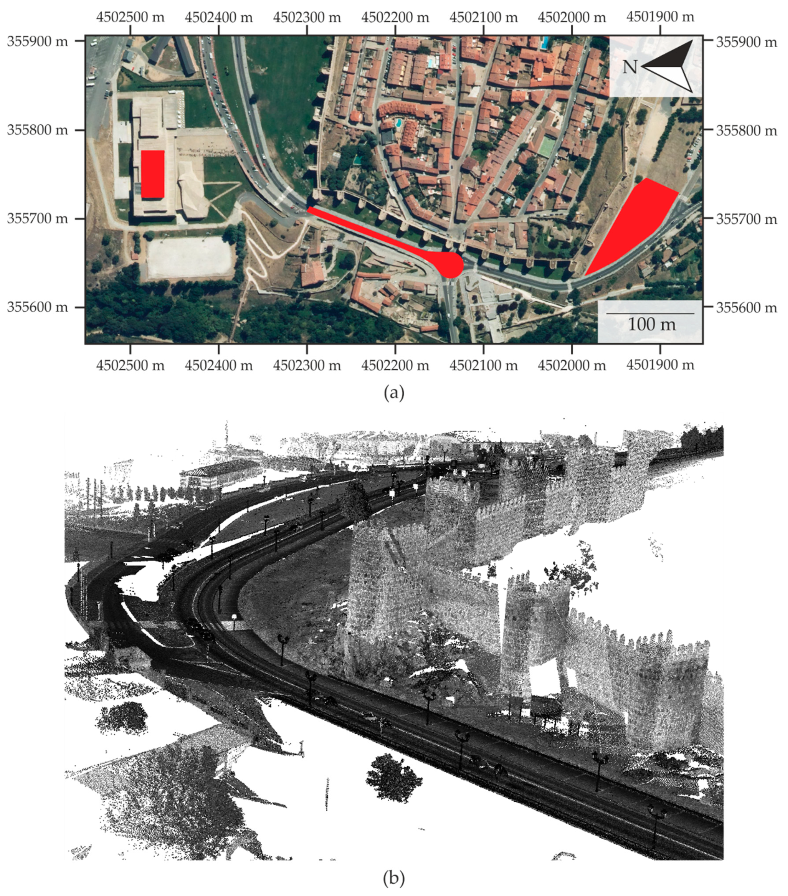
In this section, some examples of the proposed method are presented using the data described in Section 2. In particular, three different test bed sites (study cases) in terms of roughness and slope (infrastructure, urban and natural) were used to validate the positional accuracy of the ALS. The examples are developed for 1D and 3D cases, but the methods for handling of any other cases are similar (e.g., 2D). For simplicity, all the examples are developed using two metric tolerances: $T_1$ and $T_2$. $T_1$ is linked to a 50% proportion of error cases, and $T_2$ is linked to a 90% proportion of error cases.

To demonstrate the validity of the proposed method, two analyses are performed: the first one is focused on the type I error (risked by the producer/the significance of the test) and the second on the type II error (risked by the user/ the power of the test. For additional information see [38]). For the type I error analysis, three different quality controls are presented to show that the acceptance of the null hypothesis performs well. For the type II error analysis, small modifications are introduced to the tolerances to observe the null hypothesis rejection behavior of the method.

For the analysis of each quality control case, several sample sizes are used, and a simulation procedure is applied to demonstrate the proposed method. Five sampling sizes (20, 50, 100, 200, 500) were considered. These sample sizes are in the range of values that have been used in other simulation studies [39,40] on the behavior of positional accuracy control methods. For each sample size, 10,000 iterations were performed. In general, the larger the number of iterations, the more the overall results of the simulation are stable. According to [41], 10,000 iterations is a suitable number for simulations of this type. For each iteration, the proposed method was applied, and the test’s behavior was analyzed. For each quality control case and sample size, the proportion of times in which the corresponding null hypothesis has been rejected is presented as the main result. When the hypothesis is true, the percentage of rejections must be close to the value of the significance that is considered (type I error). When the hypothesis is false, the percentage of rejections is the power of the test (type II error).

3.1. Type I Error Analysis

Three different cases of quality controls are presented (QC1, QC2, QC3) to show that the method can be applied in different situations. The first two situations address the adoption of control tolerances derived from models based on normal data. The third case is based on quantiles, so its distribution is free. The proposed quality controls are as follows:

• QC1. The data are considered to be unbiased, and intervals are defined around the zero value (signed errors are considered).
• QC2. The data are considered to have bias. The bias (expressed by the median) is taken into account, and intervals are defined around the median.
• QC3. The observed quantiles are used.

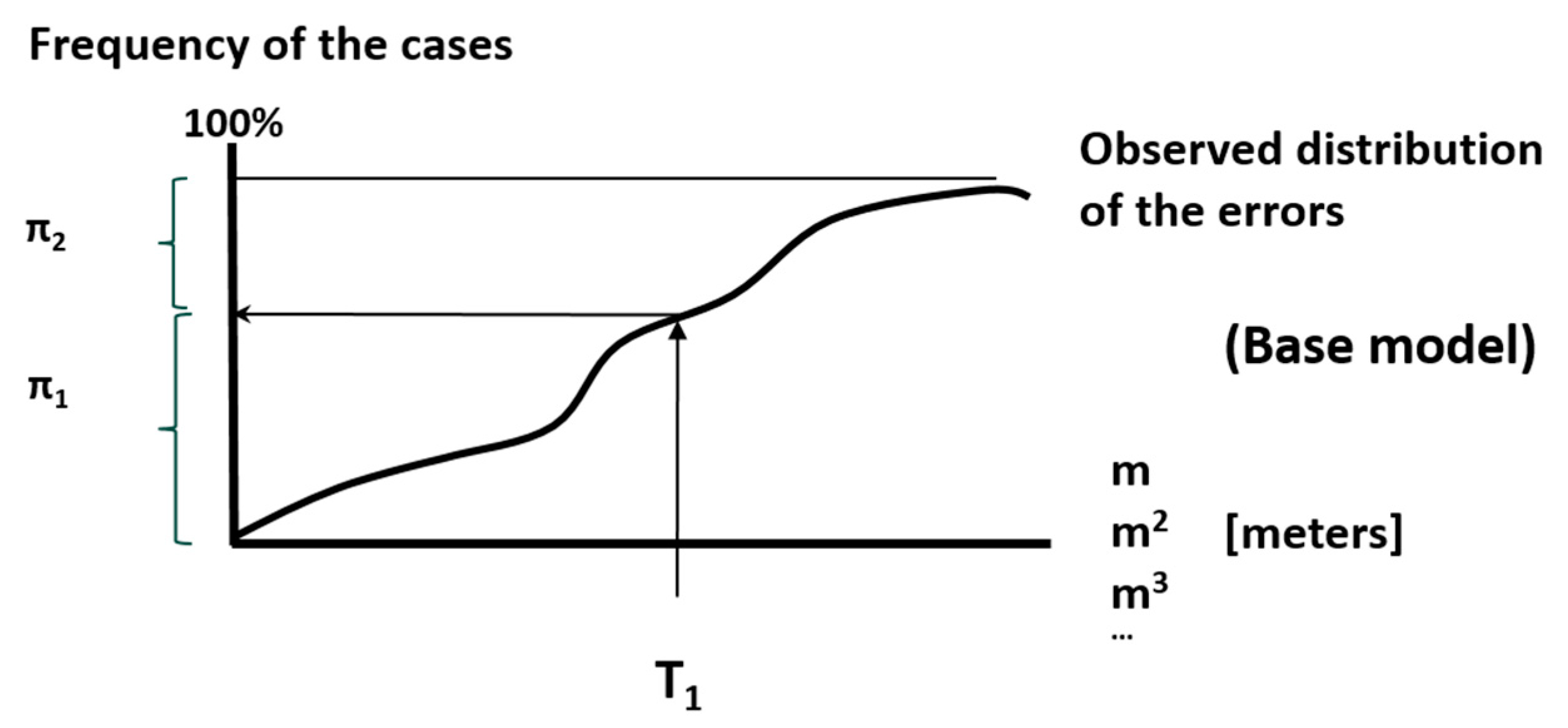
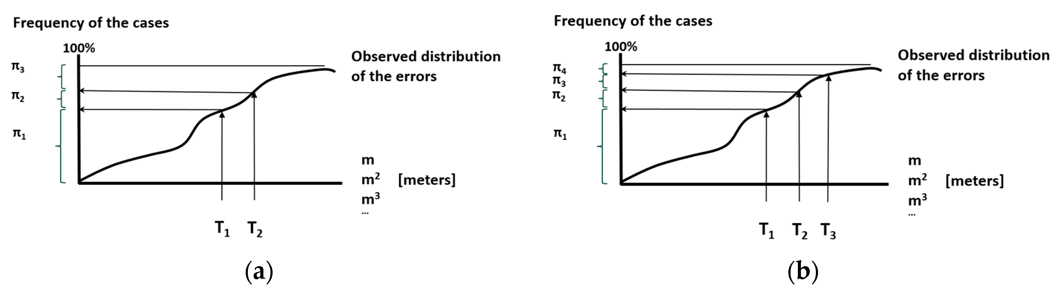
For each quality control case, the metric tolerances (thresholds) are defined based on Table 5. In all cases, tolerances define three categories of errors (CoE1, CoE2, CoE3) and account for the number of errors in each of these categories (${\nu }^{\ast }$). In all cases, the null hypothesis ${ℍ}_0$ to be tested is:

${ℍ}_0:$ The population probabilities for CoE1, CoE2 and CoE3 are, respectively ${\pi }^0=\left(0.50,0.40,0.10\right)$

Against the alternative hypothesis

${ℍ}_1:$ the true probabilities are worse than ${\pi }^0$.

3.1.1. Quality Control #1

The data are considered to be unbiased, and intervals are defined around the zero value (signed errors are considered). This situation is ideal because it is desirable that no bias is present, and it is equivalent to taking the absolute values of errors. As a guide, the tolerances are established in relation to the Gaussian model. In this situation, it is mandatory to distinguish between 1D (infrastructure) and 3D (urban and natural) cases. The tolerance values are as follows:

• For the 1D study case (infrastructure sample), since the errors were computed according to the Z discrepancies, the NMAD value is ±0.02 m. The values are derived as follows: $T_1=T_{50\%}=0.6745\times 0.020$ m and $T_2=T_{90\%}=1.6449\times 0.020$ m
• For the two 3D study cases (urban and natural samples) where the error was computed according to a 3D signed distance, a unique reference value is used via the arithmetic mean of both the NMAD (±0.088 and ±0.064 m), which is ±0.075 m, and the values derived as follows: $T_1=T_{50\%}=0.51\times \left(3\times 0.075\right)$ m and $T_2=T_{90\%}=0.833\times \left(3\times 0.075\right)$ m

Consequently, three categories of errors (CoE1..3) are defined as follows:

• Infrastructure study case. The tolerances for the 1D case define the following intervals:

  -

  CoE1: $\left|E_i\right|\in \left[0,T_1\right]=\left[0,0.0135\right]\mathrm{m}$.

  -

  CoE2: $\left|E_i\right|\in \left(T_1;T_2\right]=\left(0.0135;0.0329\right]\mathrm{m}$

  -

  CoE3: $\left|E_i\right|\in \left(T_2,\infty \right)=\left(0.0329,\infty \right)\mathrm{m}$.

• Urban and Natural study cases. The tolerances for the 3D case define the following intervals:

  -

  CoE1: $\left|E_i\right|\in \left[0,T_1\right]=\left[0,0.1147\right]\mathrm{m}$.

  -

  CoE2: $\left|E_i\right|\in (T_1,T_2]=\left(0.1147,0.1874\right]\mathrm{m}$

  -

  CoE3: $\left|E_i\right|\in T_2=\left(0.1874,\infty \right)\mathrm{m}$.

The results obtained by the simulation following the process described at the beginning of this section are shown in

Table 7. Proportion of times that the null hypothesis has been rejected for the QC1 in each study case.

		Infrastructure	Urban	Natural
Sampling size	20	0.733	0.0000	0.0037
	50	0.980	0.0000	0.0010
	100	1.000	0.0000	0.0000
	200	1.000	0.0000	0.0000
	500	1.000	0.0000	0.0000

. The situation is very clear, and the controls on the infrastructure data usually result in a rejection of the null hypothesis (i.e., the null hypothesis not accepted), even with small sample sizes. This finding implies that the proposed limits are very restrictive or, in other words, that the data do not verify the specifications. Otherwise, for the remaining two cases of study, the test always results in the acceptance of the null hypothesis. This finding implies that true limits of the errors are narrower than the specifications being considered.

3.1.2. Quality Control #2

Now, data are considered to have bias (expressed by the median, see Table 5). Intervals are built as:$Median\pm tolerance$, where the tolerances are the same as for the QC1 case.

Consequently, three categories of errors are defined:

• Infrastructure study case. The tolerances for the 1D case define the following intervals:

  -

  CoE1: $E_i\in \left[-0.039,-0.012\right]\mathrm{m}$.

  -

  CoE2: $E_i\in \left[-0.058,-0.039\right)\mathrm{m}$ OR $E_i\in \left(-0.012,0.007\right]\mathrm{m}$.

  -

  CoE3: $E_i\in \left(-\infty ,-0.058\right)\mathrm{m}$ OR $E_i\in \left(0.007,\infty \right)\mathrm{m}$

• Urban study case. The tolerances for the 3D case define the following intervals:

  -

  CoE1: $E_i\in \left[-0.179,0.050\right]\mathrm{m}$.

  -

  CoE2: $E_i\in \left[-0.252,-0.179\right)\mathrm{m}$ OR $E_i\in \left(0.050,0.123\right]\mathrm{m}$.

  -

  CoE3: $E_i\in \left(-\infty ,-0.252\right)\mathrm{m}$ OR $E_i\in \left(0.123,\infty \right)\mathrm{m}$.

• Natural study case. The tolerances for the 3D case define the following intervals:

  -

  CoE1: $E_i\in \left[-0.212,0.017\right]\mathrm{m}$.

  -

  CoE2: $E_i\in \left[-0.284,-0.212\right)\mathrm{m}$ OR $E_i\in \left(0.017,0.090\right]\mathrm{m}$.

  -

  CoE3: $E_i\in \left(-\infty ,-0.284\right)\mathrm{m}$ OR $E_i\in \left(0.090,\infty \right)\mathrm{m}$.

The results obtained by the simulation following the process described at the beginning of this section are shown in

Table 8. Proportion of times that the null hypothesis has been rejected for the QC2 (bias case).

		Infrastructure	Urban	Natural
Sampling size	20	0.0492	0.0000	0.0000
	50	0.0582	0.0000	0.0000
	100	0.0640	0.0000	0.0000
	200	0.0810	0.0000	0.0000
	500	0.1001	0.0000	0.0000

. Here, the situation is somewhat different from QC1. Study cases 2 and 3 behave almost as they did in QC1 and the null hypothesis is always accepted. Study case 1 reduces its rejection noticeably because when including the bias in the calculations, there are more error cases within the tolerances. For this study case, the rejection values are close to the significance level (5%), and this is logical since the values of the tolerances for this case are very close to the quantiles of the observed distribution (Table 5).

3.1.3. Quality Control #3

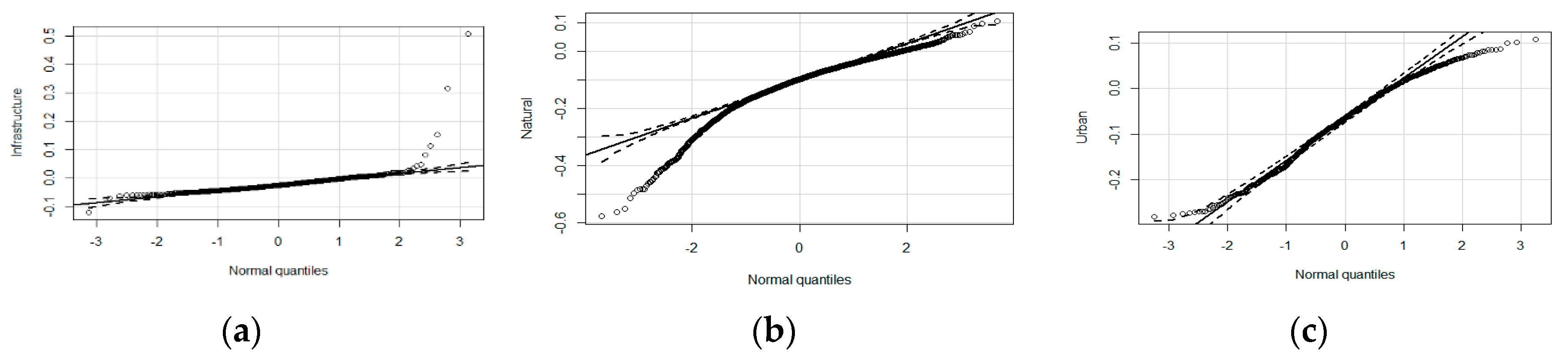
Because it has been demonstrated (see Section 2.1) that data are not normally distributed, tolerances in direct relation to quantiles can be used for quality control. In the QC3 case, the quantiles from the same error distribution function were used, which means that a high acceptance is expected. In this quality control case, the three err*or categories are determined as follows:

• CoE1: $E_i\in \left[Q_{25},Q_{75}\right]\mathrm{m}$
• CoE2: $E_i\in \left[Q_5,Q_{25}\right)\mathrm{m}$ OR $E_i\in \left(Q_{75},Q_{95}\right]\mathrm{m}$
• CoE3: $E_i\in \left[(-\infty ,Q_5\right)\mathrm{m}$ OR $E_i\in \left(Q_{95},\infty \right)\mathrm{m}$

Where the quantiles actuating as tolerances are those presented in Table 4.

The results obtained by the simulation following the process described at the beginning of this section are shown in

Table 9. Proportion of times that the null hypothesis has been rejected for the QC3 (true case).

		Infrastructure	Urban	Natural
Sampling size	20	0.0401	0.0412	0.0398
	50	0.0456	0.0492	0.0412
	100	0.0430	0.0470	0.0410
	200	0.0395	0.0360	0.0420
	500	0.0401	0.0458	0.0469

.

For the three study cases and sample sizes, the proportion of times that the null hypothesis is rejected when it actually is true is close to the significance value (α = 5%) and does not depend on the sampling size. The tolerances used in this base case of QC3 come from the observed distribution (Table 5), so that the distribution being used is its own observed probabilistic model, and therefore its probability of acceptance and the rejection level approximately equals the significance value of the hypothesis test.

In short, the interpretation of the three controls (QC1, QC2, and QC3) performed to know the type I error when the new proposed method is applied are conclusive: the proposed method allows to control this type error effectively. This is what happens in the case QC # 3, which is based on the determination of tolerances from the observed data (remember that errors do not follow a normal distribution). This situation is very different from those shown in QC1 and QC2 because in these cases, the adopted base model for deriving the tolerances was based on a Gaussian model. The QC1 and QC2 cases are a clear example that tolerances must be well established to be neither too permissive nor too restrictive in relation to the type I error. The best is that the tolerances are based on the behavior of the observed data, not on models that are supposed to follow that data (usually this is not checked). The method allows us to perfectly adjust the risk of the producer (type I error or the significance), which is an appropriate behavior with respect to the data under analysis and to the interest of quality controls. The statistical behavior of the proposed method is as expected; the observed data only show and confirm its applicability to the use case.

3.2. Type II Error Analysis

Now, we will study how the method behaves when the null hypothesis is not true; we will study the power of the statistical test. Since our proposal is specially designed for non-normal data, it is necessary to analyze the sensitivity of this method based on error counting when modifying tolerances. Considering the same situation as for QC3 (based on the observed data), we work with four extensions of the case in which the probability limits have been modified with respect to limits specified in the base case (QC3). The first two extended cases (ExC1 and ExC2) are more restrictive than the base case (QC3), and the last two extended cases (ExC3 and ExC4) are less restrictive than the base case (QC3). The newly proposed control limits of $L_j$ (in meters) appear in

Table 10. Control limits (m) for the extended cases for the 3rd quality control.

	Limits	Extended Cases
		ExC1	ExC2	ExC3	ExC4
Infrastructure	$L_5$	−0.0473	−0.0423	−0.0573	−0.0623
	$L_{25}$	−0.0334	−0.0284	−0.0434	−0.0484
	$L_{75}$	−0.0157	−0.0207	−0.0057	−0.0007
	$L_{95}$	0.0041	−0.0009	0.0141	0.0191
	Variation	+0.005	+0.01	−0.005	−0.01
Urban	$L_5$	−0.1956	−0.1756	−0.2356	−0.2556
	$L_{25}$	−0.1079	−0.0879	−0.1479	−0.1679
	$L_{75}$	−0.0255	−0.0455	0.0145	0.0345
	$L_{95}$	0.0321	0.0121	0.0721	0.0921
	Variation	+0.02	+0.04	−0.02	−0.04
Natural	$L_5$	−0.2284	−0.2084	−0.2684	−0.2884
	$L_{25}$	−0.125	−0.105	−0.165	−0.185
	$L_{75}$	−0.077	−0.097	−0.037	−0.017
	$L_{95}$	−0.03	−0.05	0.01	0.03
	Variation	+0.02	+0.04	−0.02	−0.04

for $j=5\%,25\%,75\%,95\%$.

For infrastructure data, the limits are modified by ±0.5 cm and ±1 cm in relation to the base case, and for urban and natural data, the limits are modified by ±2 cm and ±4 cm in relation to the base case. Different values are considered for the infrastructure data (0.5 cm and 1 cm) and the urban/natural data (2 cm and 4 cm) since the distribution of the error data for the first case is narrower than the other cases. In all the extended cases, the three error categories are determined as follows:

• CoE1: $E_i\in \left[L_{25},L_{75}\right]\mathrm{m}$
• CoE2: $E_i\in \left[L_5,L_{25}\right)\mathrm{m}$ OR $E_i\in \left(L_{75},L_{95}\right]\mathrm{m}$
• CoE3: $E_i\in \left(-\infty ,L_5\right)\mathrm{m}$ OR $E_i\in \left(L_{95},\infty \right)\mathrm{m}$

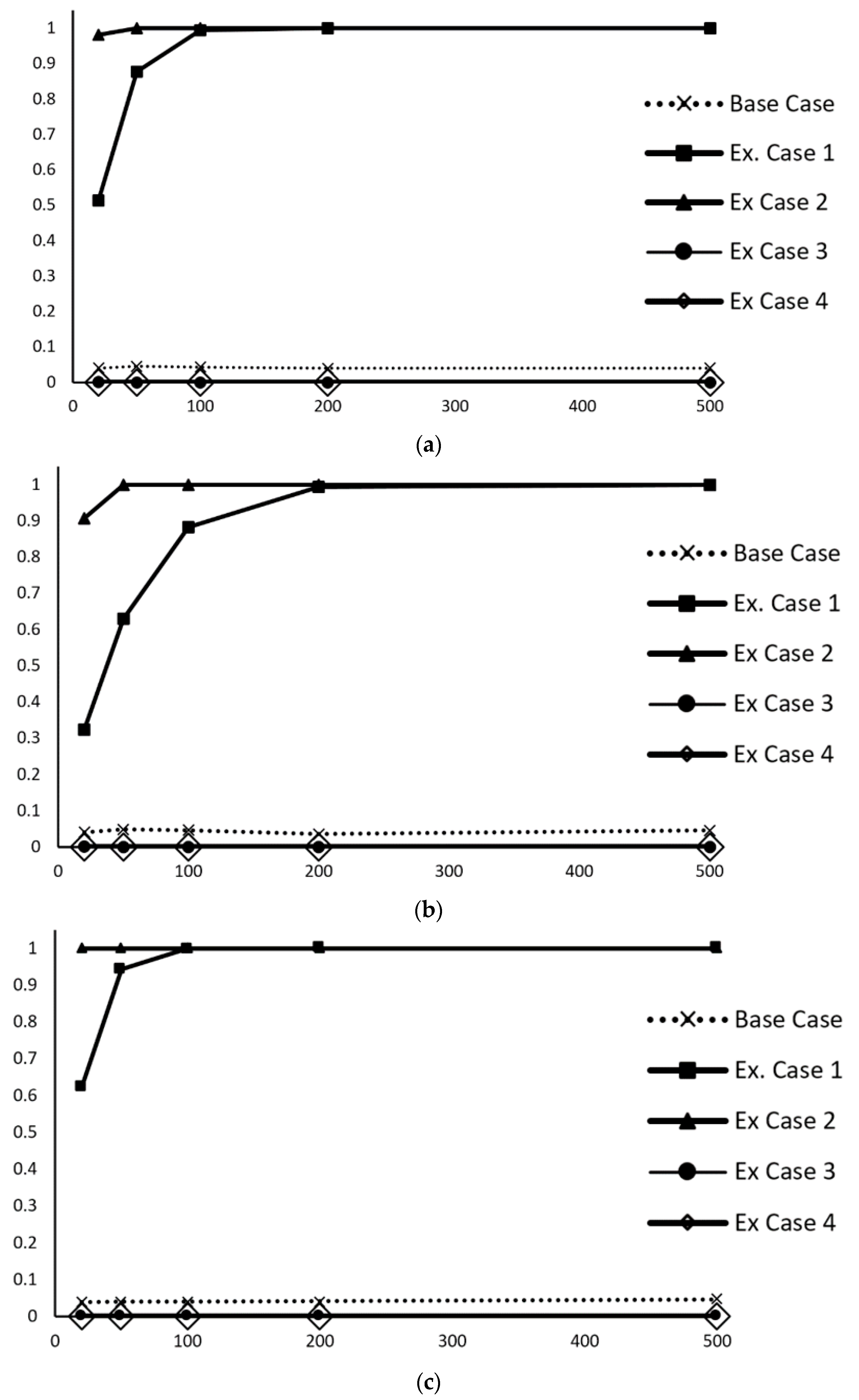
The results of this sensitivity analysis for the three study cases are shown in Figure 5. Additionally, for comparison, the base case for QC3 is included in each data category. The curves are very similar for the three study cases. In the two extended cases (ExC1 and ExC2), which are more restrictive than the base case of QC3, the null hypothesis is widely rejected even with small sample sizes (see the upper curves), whereas in the two extended cases (ExC3 and ExC4), which are less restrictive than the base case of QC3, the null hypothesis is always accepted. The curve of the base case of QC3 has been added, and it can be observed that this curve is almost horizontal, with a value of approximately 5%. This sensitivity analysis clearly shows that the method works well against variations in tolerances (statistical power or type II error). If the tolerances are more restrictive, the null hypothesis is rejected with great probability even for small sample sizes. If the tolerances are more generous, the null hypothesis is always accepted.

In conclusion, the behavior of the proposed control method is expected for a statistical contrast with respect to type II error. In addition, the example shown can guide users of the new method to test with their data and evaluate the power of the statistical contrast they are applying in their specific case.

4. Conclusions

In this paper, a new statistical method for positional accuracy quality control has been proposed, which can be applied to non-normal errors and to any number of dimensions.

The new control method is based on the use of a multinomial distribution that categorizes the cases of errors according to metric tolerances. This method of defining a quality control is very versatile and allows the control of positional errors in 1D, 2D, and 3D cases. In addition, depending on the number of tolerances considered, a greater degree of similarity could be established between the observed distribution of errors and any desired probabilistic model. The major advantages of this method are as follows:

(1) it can be applied to any kind of error model (parametric or nonparametric),

(2) it can be applied to a mix of error models (e.g., in a 3D case, the X and Y errors can be normally distributed and the Z errors can be non-normally distributed),

(3) it can be applied to any kind of geometry (e.g., points, line strings, etc.),

(4) it can be applied to cases of any dimension (1D, 2D, 3D, …nD),

(5) the method allows quantitative and qualitative aspects to be jointly controlled by means of proportions in established categories.

The method has been proposed in a generic way and has been developed for the case of two tolerances (three categories of errors). The most complex aspect of the method is that it is an exact test, so the calculation of the p-value is not done by means of approximations but by calculating the sum of a finite set of solutions. In the appendix, an example is presented to show how to calculate the p-value using the R statistical program. This test is very flexible because the specification limits, the probabilities for each category and even the dimension number can be established by the user.

To demonstrate the applicability, ALS data from three different study cases (infrastructure, urban and natural) have been used, and 1D and 3D errors have been considered. Three quality controls with different tolerances were applied. In two of the quality control cases, the tolerances were defined from a Gaussian model (with and without bias), and in the third quality control case, the tolerances were defined from the quantiles of the observed error distribution.

The results of the three study cases and of the three quality controls show that if tolerances are well established for in the control of positional accuracy, problems of excess rejection or of excess acceptance can occur. For the case of non-normal data, the use of quantiles is suggested to establish the values of the metric tolerances. The quality controls developed by simulation for the three study cases and for different sample sizes show that this method is capable of ensuring the desired significance level. In addition, the sensitivity analysis carried out by modifying the tolerances indicates that the statistical power of the new proposed control method is adequate since correct results are obtained, and they are quite stable for sample sizes greater than 100.

Taking into account the results according to the variability of the study cases, the proposed method is very promising to improve the quality control of ALS data and other non-normally distributed spatial datasets, which is the usual case when we deal with in geotechnologies, such as terrestrial laser scanning or photogrammetry.

References

1. Chen, Z.; Gao, B.; Devereux, B. State-of-the-art: DTM generation using airborne LIDAR data. Sensors 2017, 17, 150. [Google Scholar] [CrossRef] [PubMed]
2. Salach, A.; Bakuła, K.; Pilarska, M.; Ostrowski, W.; Górski, K.; Kurczyński, Z. Accuracy assessment of point clouds from LidaR and dense image matching acquired using the UAV platform for DTM creation. ISPRS Int. J. Geo-Inf. 2018, 7, 342. [Google Scholar] [CrossRef]
3. Parente, C.; Pepe, M. Uncertainty in Landslides Volume Estimation Using DEMs Generated by Airborne Laser Scanner and Photogrammetry Data. Int. Arch. Photogramm. Remote Sens. Spat. Inf. Sci. 2018, 42(3/W4), 397–404. [Google Scholar] [CrossRef]
4. Simpson, J.; Smith, T.; Wooster, M. Assessment of errors caused by forest vegetation structure in airborne LiDAR-derived DTMs. Remote Sens. 2017, 9, 1101. [Google Scholar] [CrossRef]
5. Stereńczak, K.; Ciesielski, M.; Balazy, R.; Zawiła-Niedźwiecki, T. Comparison of various algorithms for DTM interpolation from LIDAR data in dense mountain forests. Eur. J. Remote Sens. 2016, 49, 599–621. [Google Scholar] [CrossRef]
6. Zahs, V.; Hämmerle, M.; Anders, K.; Hecht, S.; Sailer, R.; Rutzinger, M.; Höfle, B. Multi-temporal 3D point cloud-based quantification and analysis of geomorphological activity at an alpine rock glacier using airborne and terrestrial LiDAR. Permafr. Periglac. Process. 2019, 30, 222–238. [Google Scholar] [CrossRef]
7. Resop, J.P.; Lehmann, L.; Hession, W.C. Drone Laser Scanning for Modeling Riverscape Topography and Vegetation: Comparison with Traditional Aerial Lidar. Drones 2019, 3, 35. [Google Scholar] [CrossRef]
8. Federal Geographic Data Committee. FGDC-STD-007: Geospatial Positioning Accuracy Standards, Part 3. National Standard for Spatial Data Accuracy; Federal Geographic Data Committee: Reston, VA, USA, 1998; p. 28.
9. American Society of Civil Engineers. Map Uses, Scales and Accuracies for Engineering and Associated Purposes; American Society of Civil Engineers; Committee on Cartographic Surveying, Surveying and Mapping Division: New York, NY, USA, 1983; p. 168. [Google Scholar]
10. STANAG. Standardization Agreement 2215: Evaluation of Land Maps, Aeronautical Charts and Digital Topographic Data; North Atlantic Treaty Organization: Bruxelles, BE, USA, 2002. [Google Scholar]
11. American Society for Photogrammetry and Remote Sensing. ASPRS Positional Accuracy standards for digital Geospatial Data. Photogramm. Eng. Remote Sens. 2015, 81, 53–63. [Google Scholar]
12. Höhle, J.; Potuckova, M. Assessment of the Quality of Digital Terrain Models; Report No. 60; European Spatial Data Research: Frankfurt, Germany, 2011. [Google Scholar]
13. Ariza-López, F.J.; Atkinson-Gordo, A.D. Analysis of some Positional Accuracy Assessment Methodologies. Surv. Eng. 2008, 134, 45–54. [Google Scholar] [CrossRef]
14. Maune, D.F. Digital Elevation Model Technologies and Applications: The Dem User’s Manual; American Society for Photogrammetry and Remote Sensing: Bethesda, MD, USA, 2007; p. 655. ISBN 978-1-57083-082-2. [Google Scholar]
15. Zandbergen, P.A. Positional Accuracy of Spatial Data: Non-Normal Distributions and a Critique of the National Standard for Spatial Data Accuracy. Trans. GIS 2008, 12, 103–130. [Google Scholar] [CrossRef]
16. Zandbergen, P.A. Characterizing the error distribution of Lidar elevation data for North Carolina. Int. J. Remote Sens. 2011, 32, 409–430. [Google Scholar] [CrossRef]
17. Liu, X.; Hu, P.; Hu, H.; Sherba, J. Approximation Theory Applied to DEM Vertical Accuracy Assessment. Trans. GIS 2012, 16, 397–410. [Google Scholar] [CrossRef]
18. Rodríguez-Gonzálvez, P.; Garcia-Gago, J.; Gomez-Lahoz, J.; González-Aguilera, D. Confronting passive and active sensors with non-gaussian statistics. Sensors 2014, 14, 13759–13777. [Google Scholar] [CrossRef] [PubMed]
19. Rodríguez-Gonzálvez, P.; González-Aguilera, D.; Hernández-López, D.; González-Jorge, H. Accuracy assessment of airborne laser scanner dataset by means of parametric and non-parametric statistical methods. IET Sci. Meas. Technol. 2015, 9, 505–513. [Google Scholar] [CrossRef]
20. Glass, G.V.; Peckham, P.D.; Sanders, J.R. Consequences of failure to meet assumptions underlying the fixed effects analyses of variance and covariance. Rev. Educ. Res. 1972, 42, 237–288. [Google Scholar] [CrossRef]
21. Berman, J. Principles of Big Data. Preparing, Sharing, and Analyzing Complex Information; Morgan Kaufmann: Burlington, MA, USA, 2013. [Google Scholar]
22. Ariza-López, F.J.; Rodríguez-Avi, J. A Statistical Model Inspired by the National Map Accuracy Standard. Photogramm. Eng. Remote Sens. 2014, 80, 271–281. [Google Scholar] [CrossRef]
23. United States Bureau of the Budget. United States National Map Accuracy Standards; United States Bureau of the Budget: Washington, DC, USA, 1947.
24. Cheok, G.; Filliben, J.; Lytle, A.M. NISTIR 7638. Guidelines for Accepting 2D Building Plans; National Institute of Standards and Technology: Gaithersburg, MD, USA, 2008. [CrossRef]
25. Ariza-López, F.J.; Rodríguez-Avi, J. A method of positional quality control testing for 2D and 3D line strings. Trans. GIS 2015, 19, 480–492. [Google Scholar] [CrossRef]
26. Asociación Española de Normalización. UNE 148002: 2016 Metodología de Evaluación de la Exactitud Posicional de la Información Geográfica; Asociación Española de Normalización: Madrid, España, 2016; p. 48. [Google Scholar]
27. International Organization for Standardization. ISO 2859-2:1985. Sampling Procedures for Inspection by Attributes—Part 2: Sampling Plans Indexed by Limiting Quality (LQ) for Isolated Lot Inspection; ISO: Genebre, Switzerland, 1985. [Google Scholar]
28. Puente, I.; González-Jorge, H.; Martínez-Sáchez, J.; Arias, P. Review of mobile mapping and surveying systems. Measurement 2013, 46, 2127–2145. [Google Scholar] [CrossRef]
29. CloudCompare. CloudCompare Version 2.9.1. [GPL Software]. Available online: http://www.cloudcompare.org (accessed on 28 February 2018).
30. Gel, Y.R.; Gastwirth, J.L. A robust modification of the Jarque–Bera test of normality. Econ. Lett. 2008, 99, 30–32. [Google Scholar] [CrossRef]
31. Hui, W.; Gel, Y.R.; Gastwirth, J.L. Lawstat: An R package for law, public policy and biostatistics. J. Stat. Softw. 2008, 28, 1–26. [Google Scholar] [CrossRef]
32. Nocerino, E.; Menna, F.; Remondino, F.; Toschi, I.; Rodríguez-Gonzálvez, P. Investigation of indoor and outdoor performance of two portable mobile mapping systems. VideometricsRange ImagingAppl. XIV 2017, 10332, 103320I. [Google Scholar]
33. Höhle, J.; Höhle, M. Accuracy assessment of digital elevation models by means of robust statistical methods. ISPRS J. Photogramm. Remote Sens. 2009, 64, 398–406. [Google Scholar] [CrossRef] [Green Version]
34. International Organization for Standardization. ISO 19157: 2013. Geographic Information. Data Quality; ISO: Genebre, Switzerland, 2013. [Google Scholar]
35. Mehta, C.R.; Patel, N.R. A Network Algorithm for Performing Fisher’s Exact Test in r×c Contingency Tables. J. Am. Stat. Assoc. 1983, 78, 427–434. [Google Scholar] [CrossRef]
36. Storer, B.E.; Choongrak, K. Exact properties of some exact test statistics for comparing two binomial proportions. J. Am. Stat. Assoc. 1990, 85, 146–155. [Google Scholar] [CrossRef]
37. Fisher, R.A. The Design of Experiments; Oliver Boyd: Edinburgh, UK, 1935. [Google Scholar]
38. Rohatgi, V.K. Statistical Inference; Dover Publications: Mineola, NY, USA, 2003; pp. 212–215. [Google Scholar]
39. Ariza-López, F.J.; Atkinson-Gordo, A.D. Variability of NSSDA estimations. Surv. Eng. 2008, 134, 404–407. [Google Scholar]
40. Ariza-López, F.J.; Atkinson-Gordo, A.D.; Rodríguez-Avi, J. Acceptance curves for the positional control of geographic data bases. Surv. Eng. 2008, 134, 26–32. [Google Scholar] [CrossRef]
41. Mundform, D.J.; Schaffer, J.; Kim, M.J.; Shaw, D.; Thongteeraparp, A.; Supawan, P. Number of Replications Required in Monte Carlo Simulation Studies: A Synthesis of Four Studies. J. Mod. Appl. Stat. Methods 2011, 10, 4. [Google Scholar] [CrossRef]
42. R Core Team. R: A Language and Environment for Statistical Computing; R Foundation for Statistical Computing: Vienna, Austria, 2018. [Google Scholar]
Figure 1. (a) Tests bed sites used in the analysis (in red), from left to right: urban (building), infrastructure (road) and natural (hillside). (b) point cloud image from airborne laser scanner (ALS).
Applsci 09 03887 g001
Figure 2. QQ-plots for the error in each study case: (a) Infrastructure, (b) Natural and (c) Urban.
Applsci 09 03887 g002
Figure 3. Key elements of a control by proportions.
Applsci 09 03887 g003
Figure 4. Conceptual example of a control by proportions: 2 tolerances (a) and three tolerances (b).
Applsci 09 03887 g004
Figure 5. Proportion of times that the null hypothesis is rejected (type II error) for the sensitivity analysis of the 3rd quality control case: (a) infrastructure study case, (b) urban study case, and (c) natural study case.
Applsci 09 03887 g005