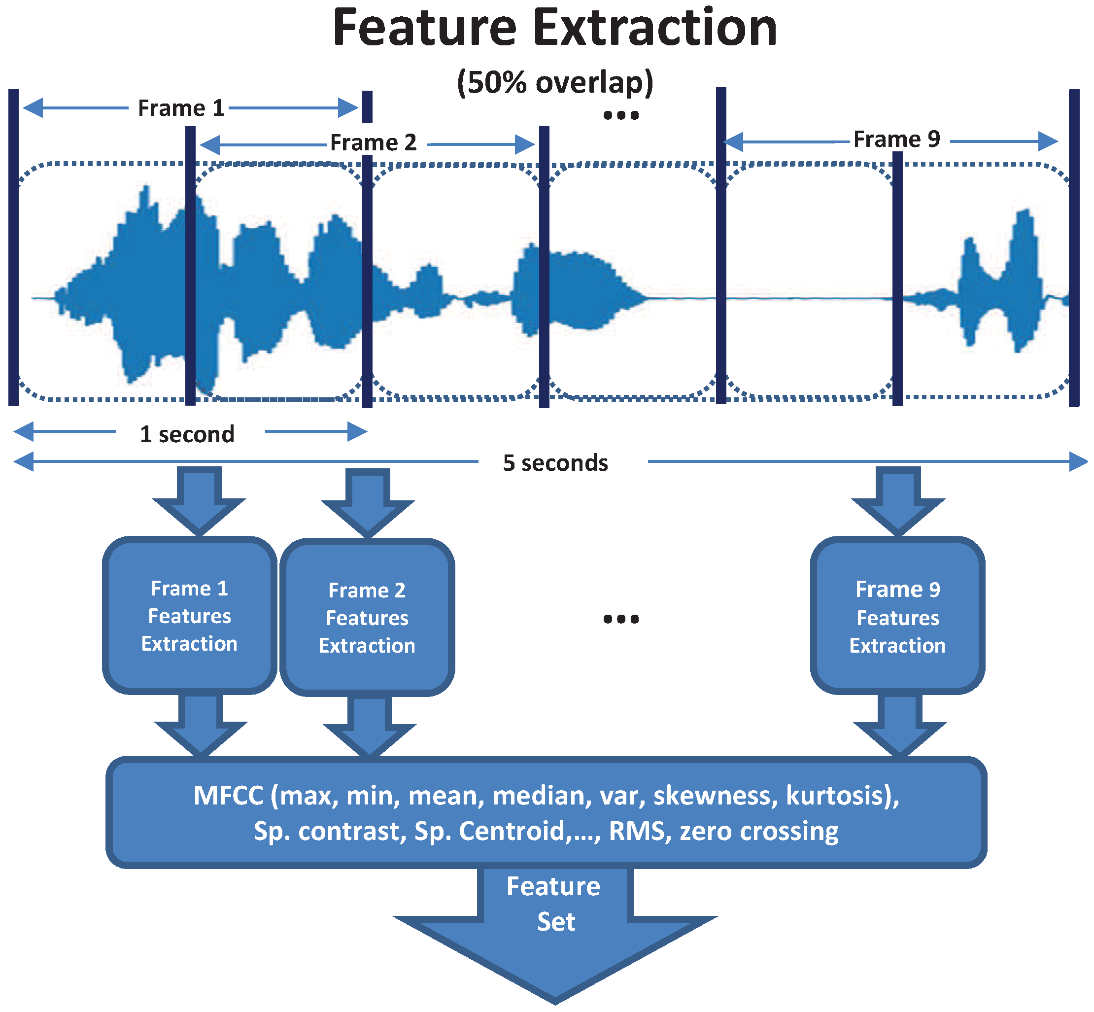
Figure 1.
A 5-second input audio signal is split in frames of one second with a 50% overlap. Each frame is sampled at 44.1 kHz and a set of audio features are extracted.
Figure 1.
A 5-second input audio signal is split in frames of one second with a 50% overlap. Each frame is sampled at 44.1 kHz and a set of audio features are extracted.
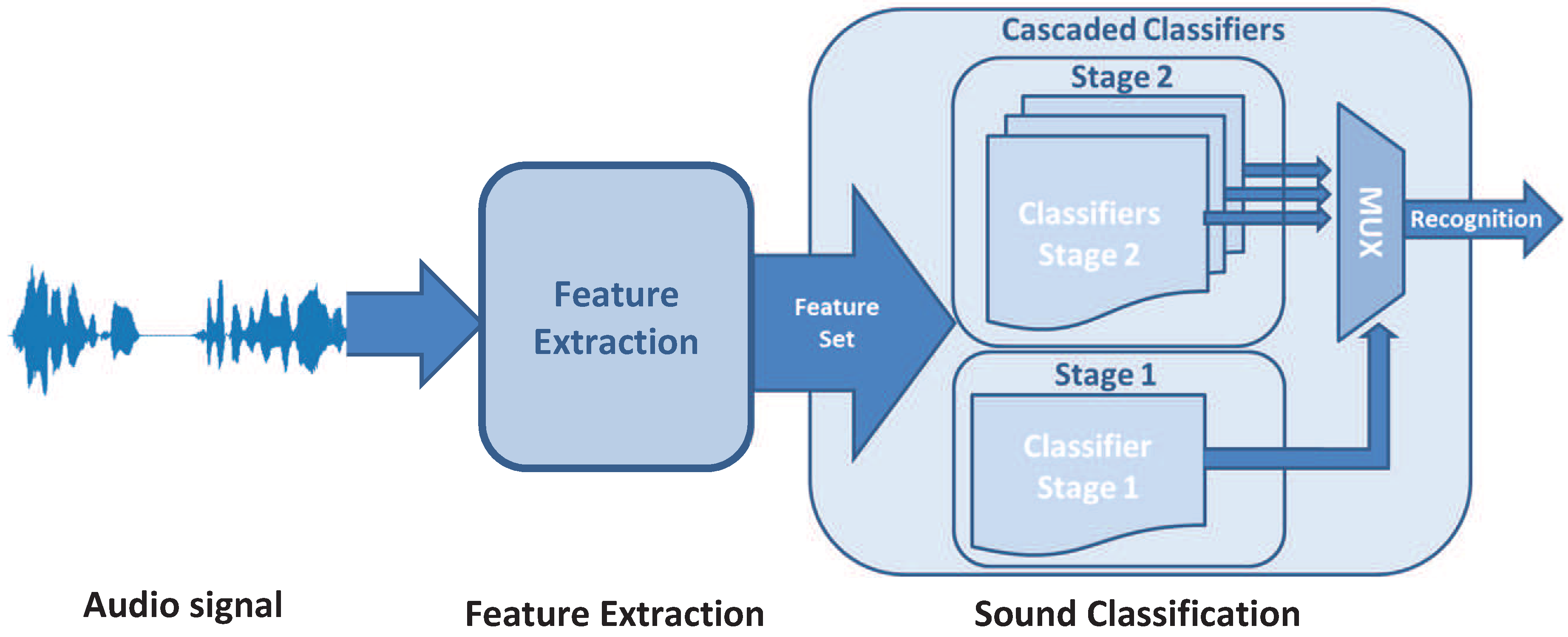
Figure 2.
The multi-stage sound classification is composed of two stages, an initial stage performs the broad classification, while a bank of classifiers are used to determine the sound’s category.
Figure 2.
The multi-stage sound classification is composed of two stages, an initial stage performs the broad classification, while a bank of classifiers are used to determine the sound’s category.
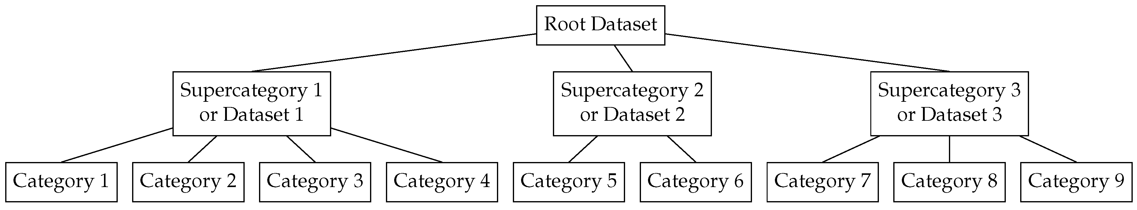
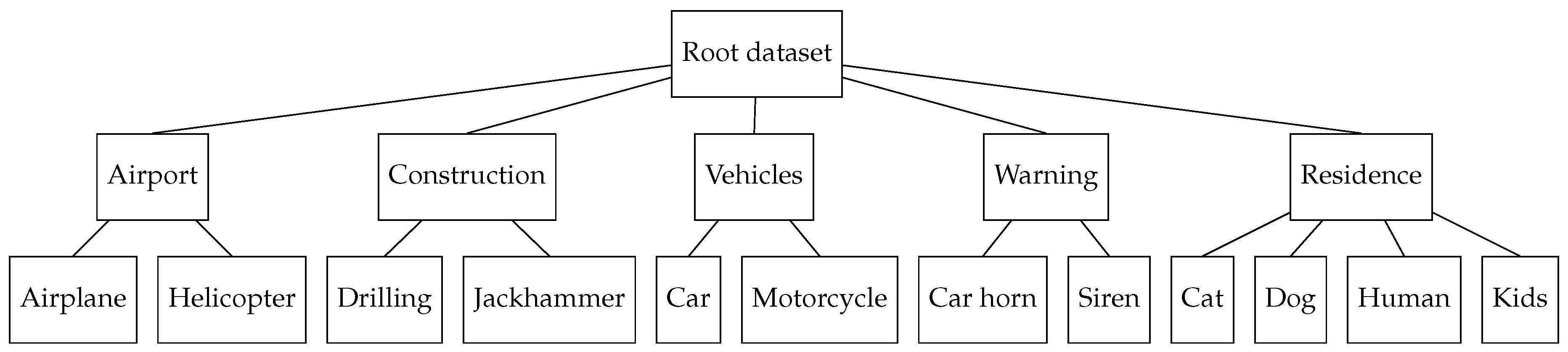
Figure 3.
Example of a hierarchical dataset to be used by our cascade approach.
Figure 3.
Example of a hierarchical dataset to be used by our cascade approach.
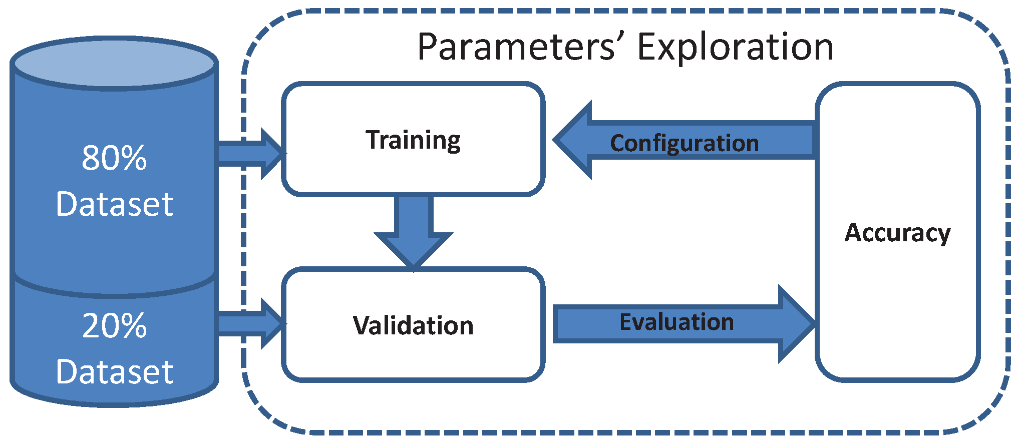
Figure 4.
The configuration of the sound classifier is selected based on the achieved accuracy.
Figure 4.
The configuration of the sound classifier is selected based on the achieved accuracy.
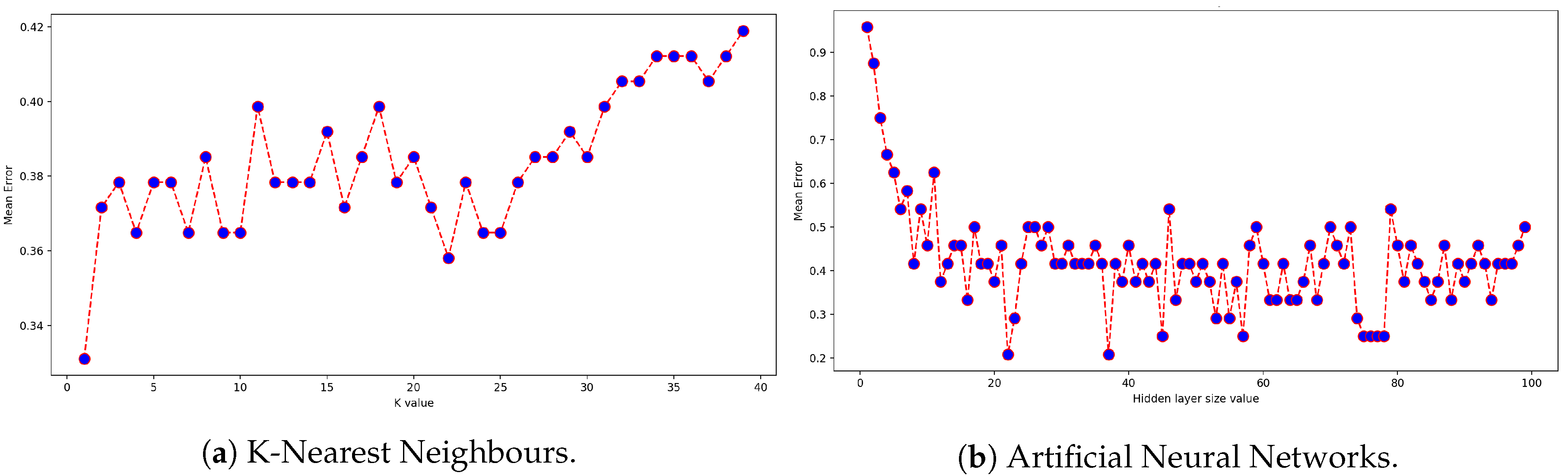
Figure 5.
Exploration of the classifiers’ parameters for the BDLib dataset. The k-NN and ANN classifiers are optimized by selecting the value of the parameter leading to the minimal mean error.
Figure 5.
Exploration of the classifiers’ parameters for the BDLib dataset. The k-NN and ANN classifiers are optimized by selecting the value of the parameter leading to the minimal mean error.
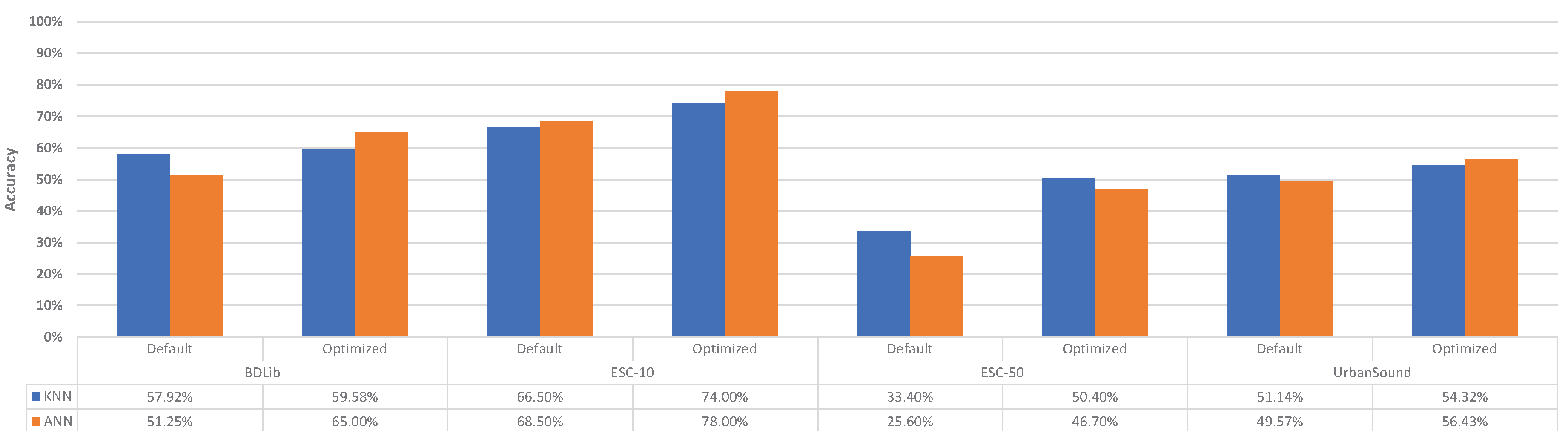
Figure 6.
Achieved accuracy of the classifiers with their default and optimized configuration.
Figure 6.
Achieved accuracy of the classifiers with their default and optimized configuration.
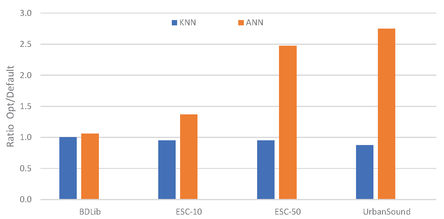
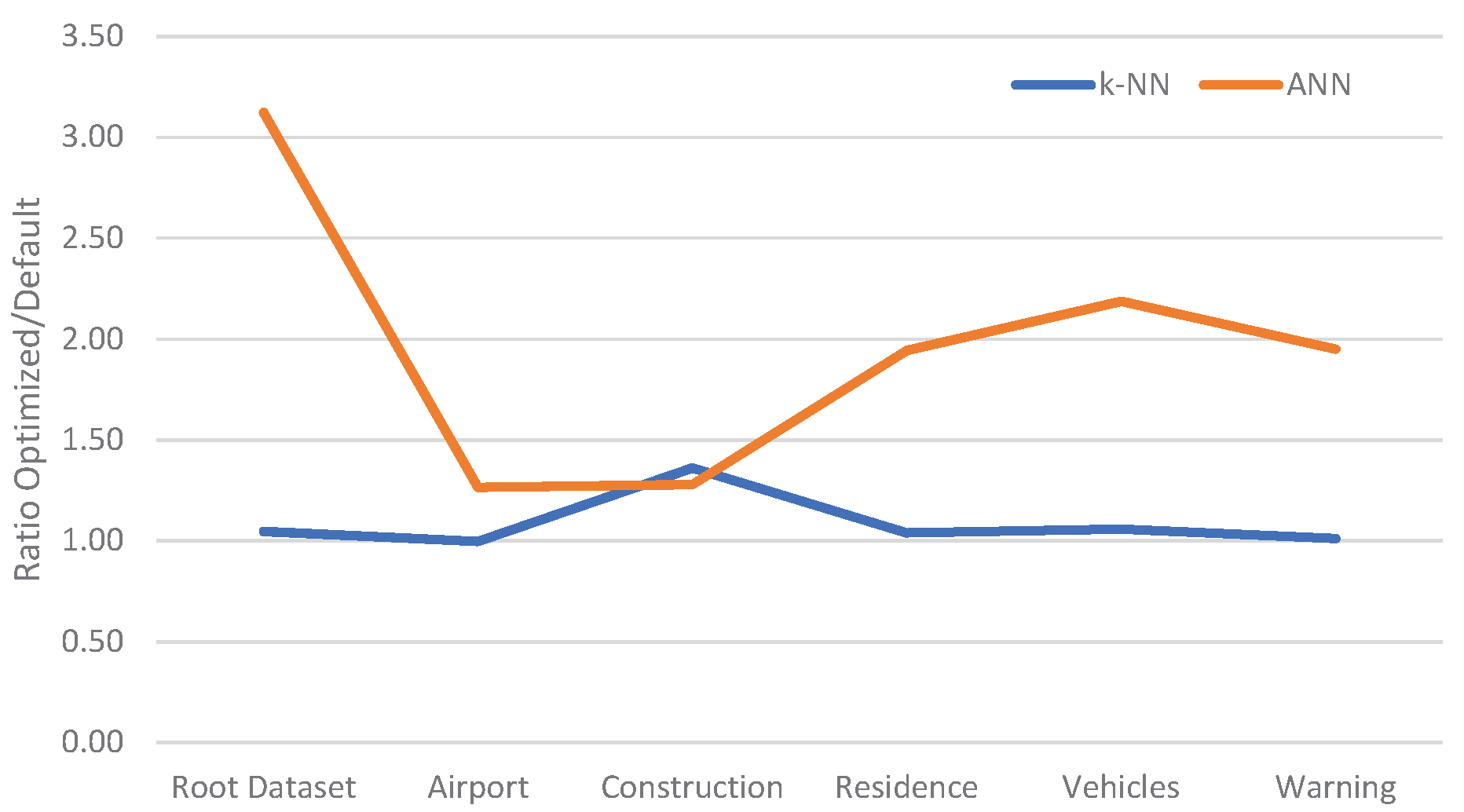
Figure 7.
Relative improvement of optimised parameters over default parameters of the classifiers.
Figure 7.
Relative improvement of optimised parameters over default parameters of the classifiers.
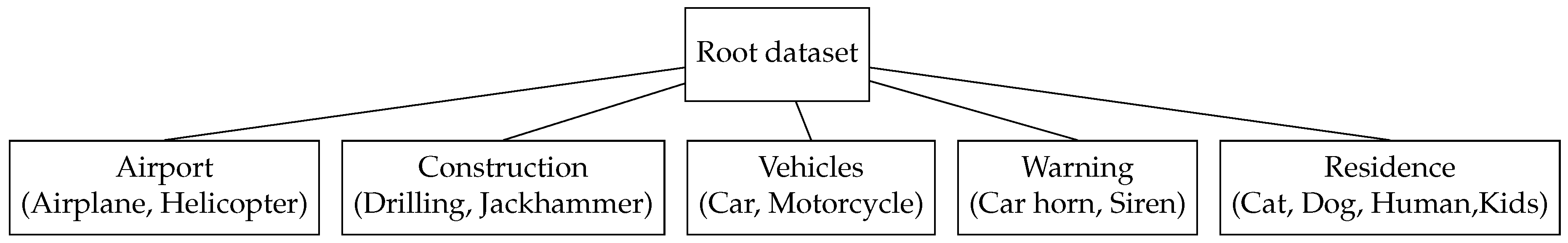
Figure 8.
Training dataset for the first stage of the cascade approach. Notice that different sound categories (in brackets) are grouped in the same category.
Figure 8.
Training dataset for the first stage of the cascade approach. Notice that different sound categories (in brackets) are grouped in the same category.
Figure 9.
Detailed hierarchical dataset for the cascade approach.
Figure 9.
Detailed hierarchical dataset for the cascade approach.
Figure 10.
Average timing of the classifiers running with their default configuration.
Figure 10.
Average timing of the classifiers running with their default configuration.
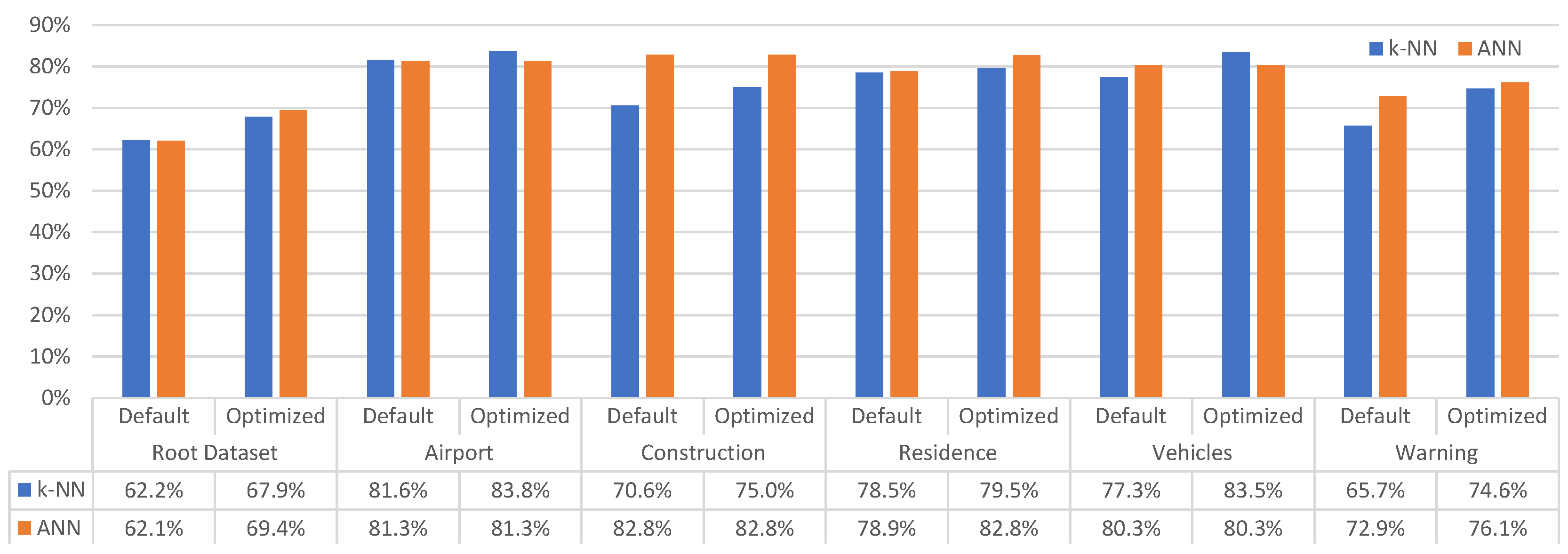
Figure 11.
Achieved accuracy of the classifiers with their default and optimized configuration.
Figure 11.
Achieved accuracy of the classifiers with their default and optimized configuration.
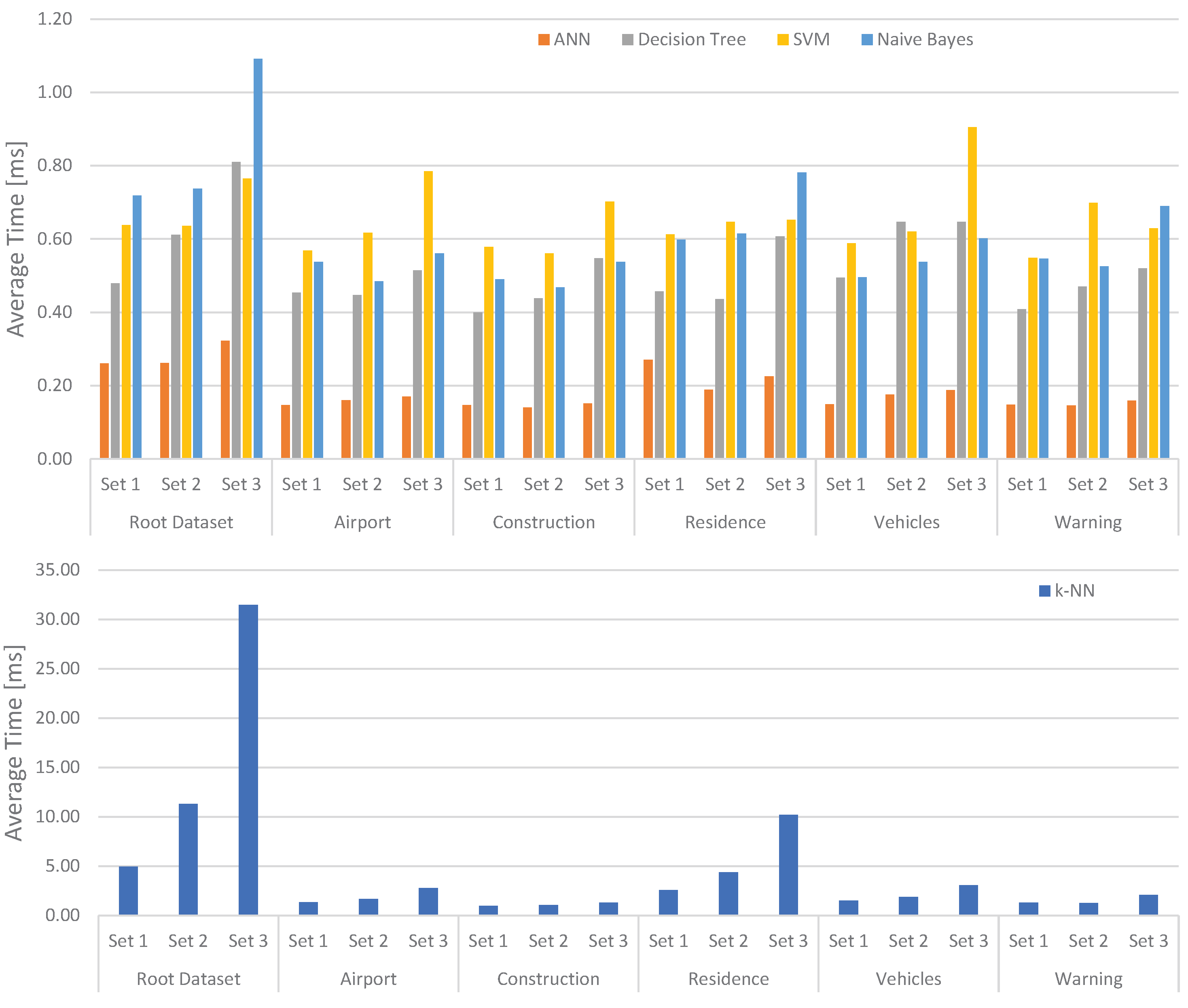
Figure 12.
Average execution time of the classifiers based on their configuration.
Figure 12.
Average execution time of the classifiers based on their configuration.
Table 1.
Details of the most popular open source datasets for urban sound and ESR.
Table 1.
Details of the most popular open source datasets for urban sound and ESR.
| BDLib Dataset | ESC-10 Dataset | UrbanSound Dataset |
|---|
| Categories | Total Time (s) | Categories | Total Time (s) | Categories | Total Time (s) |
|---|
| Airplane | 100 | Dog barking | 200 | Air conditioner | 6577 |
| Alarms | 100 | Baby crying | 200 | Car horn | 4819 |
| Applause | 100 | Clock tick | 200 | Children playing | 13454 |
| Birds | 100 | Person sneezing | 200 | Dog bark | 8399 |
| Dogs | 100 | Helicopter | 200 | Drilling | 4864 |
| Footsteps | 100 | Chainsaw | 200 | Engine idling | 3604 |
| Motorcycles | 100 | Rooster | 200 | Gun shot | 7865 |
| Rain | 100 | Fire cracking | 200 | Jackhammer | 4328 |
| Sea waves | 100 | Sea waves | 200 | Siren | 4477 |
| Wind | 100 | Rain | 200 | Street music | 6453 |
| Rivers | 100 | | |
| Thunderstorm | 100 | | |
Table 2.
List of some libraries for audio analysis. The selected library is highlighted in bold.
Table 2.
List of some libraries for audio analysis. The selected library is highlighted in bold.
| Name | Language | Description |
|---|
| pyAudioAnalysis [19,20] | Python | Audio Feature Extraction and Classification |
| Yaafe [21] | Python | Audio Feature Extraction |
| Essentia [18,22] | C++ | Audio Feature Extraction and Classification |
| aubio [23] | C | Audio Feature Extraction |
| CLAM [24] | C++ | Audio Feature Extraction |
| LibROSA [25,26] | Python | Audio Feature Extraction |
| Matlab Audio Analysis Library [27] | Matlab | Audio Feature Extraction and Classification |
| PyCASP [28,29] | Python | Audio-Specialized library for automatic
mapping of computations onto
GPUs or multicore CPUs. |
| seewave [30] | R | Audio Feature Extraction |
| bob [31,32] | C++/Python | Audio Feature Extraction and Classification |
Table 3.
Classifiers’ accuracy per dataset reported in the literature.
Table 3.
Classifiers’ accuracy per dataset reported in the literature.
| Classifier | BDLib [1] | ESC-10 [2] | ESC-50 [2] | UrbanSound [3] |
|---|
| k-NN | 45.5% | 66.7% | 32.2% | - |
| Naive Bayes | 45.9% | - | - | - |
| ANN | 54.0% | - | - | - |
| SVM | 53.7% | 67.5% | 39.9% | ≈70% |
| Decision Trees | - | - | - | ≈48% |
Table 4.
Measured classifiers’ accuracy per dataset and average execution time of the classifiers with default configuration. Accuracy and timing values are expressed in percentage and milliseconds, respectively. The values in brackets are the Standard Deviation (SD).
Table 4.
Measured classifiers’ accuracy per dataset and average execution time of the classifiers with default configuration. Accuracy and timing values are expressed in percentage and milliseconds, respectively. The values in brackets are the Standard Deviation (SD).
| Classifier | BDLib | ESC-10 | ESC-50 | UrbanSound |
|---|
| Accuracy [%] | Timing [ms] | Accuracy [%] | Timing [ms] | Accuracy [%] | Timing [ms] | Accuracy [%] | Timing [ms] |
|---|
| k-NN | 59.58 (15.22) | 1.98 (0.69) | 73.50 (6.26) | 1.54 (0.44) | 46.90 (4.41) | 15.13 (0.59) | 42.83 (8.09) | 5.91 (0.17) |
| Naive Bayes | 62.08 (14.76) | 1.04 (0.06) | 69.50 (8.64) | 0.95 (0.09) | 45.00 (5.01) | 5.38 (0.69) | 53.50 (5.74) | 1.21 (0.15) |
| ANN | 52.92 (12.27) | 0.18 (0.02) | 67.50 (8.89) | 0.19 (0.08) | 21.20 (2.82) | 0.35 (0.06) | 39.17 (4.73) | 0.22 (0.01) |
| SVM | 30.00 (8.52) | 0.71 (0.19) | 40.00 (12.47) | 0.73 (0.25) | 11.80 (4.05) | 0.92 (0.11) | 29.17 (4.86) | 0.65 (0.07) |
| Decision Trees | 29.17 (10.21) | 0.55 (0.07) | 39.00 (8.09) | 0.54 (0.08) | 7.50 (2.37) | 0.67 (0.04) | 26.50 (4.74) | 0.64 (0.05) |
Table 5.
Optimal values of the classifiers’ parameters which minimize the accuracy error per dataset.
Table 5.
Optimal values of the classifiers’ parameters which minimize the accuracy error per dataset.
| Classifier | Parameter | Default | BDLib | ESC-10 | ESC-50 | UrbanSound |
|---|
| k-NN | n_neighbours | 5 | 1 | 1 | 1 | 1 |
| ANN | hidden layer | 10 | 39 | 23 | 87 | 88 |
Table 6.
Summary of the categories used in the hierarchical dataset.
Table 6.
Summary of the categories used in the hierarchical dataset.
| Datasets | Categories | Audio Data (s) |
|---|
| Root Dataset | Airport | 475 |
| Traffic | 475 |
| Construction | 475 |
| Residence | 475 |
| Airport | Airplane | 395 |
| Helicopter | 395 |
| Construction | Drilling | 170 |
| Jackhammer | 170 |
| Vehicles | Cars | 455 |
| Motorcycles | 455 |
| Warning | Cars horn | 345 |
| Siren | 345 |
| Residence | Cats | 505 |
| Human | 505 |
| Children | 505 |
| Dogs | 505 |
Table 7.
Considered feature sets and average time required for the features’ extraction. The values in brackets are the Standard Deviation (SD).
Table 7.
Considered feature sets and average time required for the features’ extraction. The values in brackets are the Standard Deviation (SD).
| Set 1 | Set 2 | Set 3 |
|---|
| Features | Time [ms] | Features | Time [ms] | Features | Time [ms] |
| Mfcc 1, 6 | 17.30 (1.08) | Zero Crossing | 4.17 (0.37) | Mfcc 0 - Mfcc 12 | 17.30 (1.08) |
| Total time () | 17.30 (1.08) | Sp. Contrast 0, 2 | 24.58 (1.92) | Sp. Contrast 0 - Sp. Contrast 5 | 24.58 (1.92) |
| | | Mfcc 0, 2, 4, 5, 7 | 17.30 (1.08) | Sp. Centroid | 12.75 (0.54) |
| | | Total time () | 46.06 (0.62) | Sp. Roll off | 12.93 (0.55) |
| | | | | Sp. Bandwidth | 15.84 (0.59) |
| | | | | Rms | 63.95 (3.70) |
| | | | | Zero Crossing | 4.17 (0.37) |
| | | | | Total time () | 151.55 (1.67) |
Table 8.
Average accuracy in percentage per data set. The best classifier per data set is highlighted in bold.
Table 8.
Average accuracy in percentage per data set. The best classifier per data set is highlighted in bold.
| Datasets | Sets | k-NN | ANN | Decision Tree | SVM | Naive Bayes |
|---|
| Root dataset | Set1 | 35.61 | 52.84 | 39.93 | 25.54 | 49.19 |
| Set2 | 55.47 | 51.76 | 44.46 | 33.04 | 47.03 |
| Set3 | 62.16 | 62.09 | 48.92 | 45.68 | 54.46 |
| Airport | Set1 | 73.44 | 72.81 | 70.31 | 61.88 | 73.13 |
| Set2 | 74.38 | 76.25 | 77.50 | 65.31 | 78.13 |
| Set3 | 81.56 | 81.25 | 70.94 | 74.69 | 69.38 |
| Construction | Set1 | 70.00 | 72.78 | 72.78 | 66.67 | 81.11 |
| Set2 | 71.11 | 85.56 | 64.44 | 74.44 | 87.22 |
| Set3 | 70.56 | 82.78 | 62.22 | 68.89 | 89.44 |
| Residence | Set1 | 44.69 | 69.38 | 59.38 | 37.38 | 62.88 |
| Set2 | 65.56 | 68.25 | 64.00 | 51.38 | 68.63 |
| Set3 | 78.52 | 78.88 | 66.38 | 71.00 | 76.25 |
| Vehicles | Set1 | 66.22 | 64.32 | 67.03 | 55.14 | 66.76 |
| Set2 | 72.16 | 78.65 | 69.19 | 59.46 | 72.43 |
| Set3 | 77.30 | 80.27 | 68.92 | 73.24 | 77.84 |
| Warning | Set1 | 60.36 | 64.64 | 60.36 | 59.64 | 64.64 |
| Set2 | 66.07 | 70.00 | 58.93 | 65.00 | 63.21 |
| Set3 | 65.71 | 72.86 | 65.00 | 65.36 | 65.36 |
Table 9.
The parameters for the optimization of the k-NN and ANN classifiers for the datasets of the cascade approach and for the non-cascade approach.
Table 9.
The parameters for the optimization of the k-NN and ANN classifiers for the datasets of the cascade approach and for the non-cascade approach.
| Optimized Parameters |
|---|
| Datasets | n_neighbors | hidden_layer_sizes |
| Root Dataset | 1 | 96 |
| Airport | 1 | 14 |
| Construction | 2 | 5 |
| Residence | 1 | 48 |
| Vehicles | 1 | 60 |
| Warning | 3 | 48 |
| Non-cascade | 1 | 74 |
Table 10.
Achievable accuracy and demanded execution time for the proposed cascade approach of the classifiers. The most accurate classifier per dataset is marked in bold. The Standard Deviation (SD) is in brackets.
Table 10.
Achievable accuracy and demanded execution time for the proposed cascade approach of the classifiers. The most accurate classifier per dataset is marked in bold. The Standard Deviation (SD) is in brackets.
| | k-NN | ANN | Decision Tree | SVM | Naive Bayes |
|---|
| | Accuracy [%] | Time [ms] | Accuracy [%] | Time [ms] | Accuracy [%] | Time [ms] | Accuracy [%] | Time [ms] | Accuracy [%] | Time [ms] |
|---|
| Root Dataset | 67.91 (3.29) | 32.94 (1.74) | 69.39 (2.78) | 1.01 (0.17) | 48.92 (6.49) | 0.72 (0.133) | 45.68 (6.43) | 0.90 (0.37) | 54.46 (2.89) | 1.42 (0.85) |
| Airport | 83.75 (4.11) | 2.78 (0.65) | 79.06 (5.11) | 0.22 (0.05) | 70.94 (7.07) | 0.70 (0.15) | 74.69 (6.66) | 0.80 (0.18) | 69.38 (7.91) | 0.65 (0.16) |
| Construction | 75.00 (9.53) | 1.75 (0.58) | 81.11 (6.52) | 0.19 (0.10) | 62.22 (9.36) | 0.53 (0.14) | 68.89 (9.14) | 0.70 (0.13) | 89.44 (9.61) | 0.59 (0.11) |
| Residence | 79.50 (3.01) | 10.61 (0.33) | 82.75 (4.32) | 0.44 (0.06) | 66.38 (3.84) | 0.91 (0.48) | 71.00 (3.98) | 0.76 (0.26) | 76.25 (7.09) | 0.87 (0.09) |
| Vehicles | 83.51 (4.84) | 3.27 (0.41) | 80.00 (8.56) | 0.41 (0.25) | 68.92 (9.38) | 0.57 (0.10) | 73.24 (4.11) | 0.83 (0.34) | 77.84 (8.04) | 0.60 (0.07) |
| Warning | 74.64 (6.62) | 2.11 (0.24) | 76.07 (4.47) | 0.31 (0.06) | 65.00 (8.72) | 0.64 (0.15) | 65.36 (5.84) | 0.99 (0.74) | 65.36 (10.79) | 0.58 (0.03) |
Table 11.
Overall accuracy and timing in milliseconds of the cascade approach for the optimized k-NN and ANN classifiers. The average values are marked in bold.
Table 11.
Overall accuracy and timing in milliseconds of the cascade approach for the optimized k-NN and ANN classifiers. The average values are marked in bold.
| Feature Set | Path | k-NN | ANN | Most Accurate | Fastest |
|---|
Overall
Accuracy [%] | Time [ms] | Overall
Accuracy [%] | Time [ms] | Accuracy [%] | Time [ms] | Accuracy [%] | Time [ms] |
|---|
| Set 3 | Root Dataset => Airport | 56.87 | 35.73 | 54.86 | 1.22 | 58.12 | 3.79 | 38.68 | 0.93 |
| Root Dataset => Construction | 50.93 | 34.69 | 56.28 | 1.20 | 62.07 | 1.60 | 39.68 | 0.91 |
| Root Dataset => Residence | 53.98 | 43.56 | 57.42 | 1.44 | 57.42 | 1.44 | 40.48 | 1.15 |
| Root Dataset => Vehicles | 56.71 | 36.21 | 55.51 | 1.41 | 57.95 | 4.28 | 39.14 | 1.12 |
| Root Dataset => Warning | 50.69 | 35.05 | 52.79 | 1.32 | 52.79 | 1.32 | 37.21 | 1.03 |
| | Mean | 53.84 | 37.05 | 55.37 | 1.32 | 57.67 | 2.48 | 39.04 | 1.03 |
| | SD | 2.99 | 3.69 | 1.73 | 0.11 | 3.30 | 1.43 | 1.22 | 0.11 |
Table 12.
Classifiers’ accuracy and timing using an equivalent non-cascade dataset. The Standard Deviation (SD) is in brackets.
Table 12.
Classifiers’ accuracy and timing using an equivalent non-cascade dataset. The Standard Deviation (SD) is in brackets.
| Categories | Feature Set | k-NN | ANN | Decision Tree | SVM | Naive Bayes |
|---|
| Accuracy [%] | Timing [ms] | Accuracy [%] | Timing [ms] | Accuracy [%] | Timing [ms] | Accuracy [%] | Timing [ms] | Accuracy [%] | Timing [ms] |
|---|
| Airplane | | | | | | | | | | | |
| Helicopter | | | | | | | | | | | |
| Jackhammer | | | | | | | | | | | |
| Drilling | | | | | | | | | | | |
| Cats | | | | | | | | | | | |
| Dogs | Set 3 | 52.264 (3.88) | 16.301 (0.82) | 56.981 (6.03) | 0.804 (0.17) | 28.869 (3.91) | 0.857 (0.43) | 32.169 (6.21) | 1.063 (0.65) | 48.962 (4.48) | 1.752 (0.14) |
| Humans | | | | | | | | | | | |
| Children | | | | | | | | | | | |
| Cars | | | | | | | | | | | |
| Motorcycles | | | | | | | | | | | |
| Car horn | | | | | | | | | | | |
| Siren | | | | | | | | | | | |
Table 13.
Average time required for the feature extraction on the Raspberry Pi. The values in brackets are the Standard Deviation (SD).
Table 13.
Average time required for the feature extraction on the Raspberry Pi. The values in brackets are the Standard Deviation (SD).
| Features | Time [ms] |
|---|
| Mfcc 0 - Mfcc 12 | 622.22 (163.71) |
| Sp. Contrast 0 - Sp. Contrast 5 | 336.39 (64.87) |
| Sp. Centroid | 300.24 (52.81) |
| Sp. Roll off | 315.79 (61.37) |
| Sp. Bandwidth | 349.83 (63.33) |
| Rms | 1089.10 (260.62) |
| Zero Crossing | 64.22 (15.19) |
| Total time () | 3077.79 (125.21) |
Table 14.
Experimental values obtained in the Raspberry Pi. The classifiers’ accuracy per dataset and the average execution time of the classifiers with default configuration are measured. Timing values are expressed in milliseconds. The values in brackets are the Standard Deviation (SD).
Table 14.
Experimental values obtained in the Raspberry Pi. The classifiers’ accuracy per dataset and the average execution time of the classifiers with default configuration are measured. Timing values are expressed in milliseconds. The values in brackets are the Standard Deviation (SD).
| Classifier | BDLib | ESC-10 | ESC-50 | UrbanSound |
|---|
| Accuracy [%] | Timing [ms] | Accuracy [%] | Timing [ms] | Accuracy [%] | Timing [ms] | Accuracy [%] | Timing [ms] |
|---|
| k-NN | 59.17 (4.73) | 12.83 (8.05) | 73.50 (10.01) | 9.54 (3.39) | 48.70 (4.19) | 114.53 (5.94) | 50.48 (2.91) | 80.70 (33.21) |
| Naive Bayes | 68.33 (10.24) | 12.42 (5.29) | 69.00 (12.87) | 10.11 (3.27) | 42.10 (3.48) | 82.18 (4.42) | 49.29 (2.62) | 11.85 (4.87) |
| ANN | 50.83 (9.38) | 2.20 (0.84) | 64.50 (10.12) | 1.85 (0.57) | 20.90 (4.39) | 5.95 (0.29) | 50.6 (3.73) | 4.34 (1.72) |
| SVM | 30.00 (8.96) | 5.01 (0.22) | 36.00 (12.65) | 4.94 (0.31) | 9.40 (3.89) | 16.79 (1.07) | 25.29 (7.73) | 6.44 (2.52) |
| Decision Trees | 29.58 (8.43) | 4.36 (0.21) | 38.00 (11.34) | 4.42 (0.24) | 6.80 (2.48) | 4.85 (0.35) | 34.7 (2.09) | 6.14 (2.41) |
Table 15.
Achievable accuracy and demanded execution time for the proposed cascade approach of the classifiers running on the Raspberry Pi. The most accurate classifier per dataset is marked in bold.
Table 15.
Achievable accuracy and demanded execution time for the proposed cascade approach of the classifiers running on the Raspberry Pi. The most accurate classifier per dataset is marked in bold.
| | k-NN | ANN | Decision Tree | SVM | Naive Bayes |
|---|
| | Accuracy [%] | Time [ms] | Accuracy [%] | Time [ms] | Accuracy [%] | Time [ms] | Accuracy [%] | Time [ms] | Accuracy [%] | Time [ms] |
|---|
| Root Dataset | 66.23 (3.16) | 300.18 (33.76) | 68.63 (3.52) | 83.66 (33.62) | 47.26 (5.39) | 5.03 (0.32) | 51.30 (5.01) | 7.26 (0.54) | 53.22 (3.86) | 15.86 (0.98) |
| Airport | 85.31 (4.89) | 15.53 (2.42) | 83.75 (5.67) | 2.66 (0.88) | 74.06 (9.20) | 5.46 (2.29) | 76.25 (5.92) | 4.93 (1.60) | 73.44 (6.95) | 5.84 (0.55) |
| Construction | 69.44 (6.28) | 7.21 (0.17) | 76.11 (9.39) | 1.11 (0.06) | 61.67 (10.68) | 5.85 (2.03) | 68.89 (11.15) | 5.80 (2.10) | 83.33 (7.35) | 5.17 (0.17) |
| Residence | 75.25 (3.63) | 77.34 (4.27) | 82.75 (3.52) | 15.38 (1.19) | 70.50 (6.85) | 4.72 (0.31) | 68.63 (8.16) | 6.20 (1.76) | 74.13 (3.82) | 9.58 (0.49) |
| Vehicles | 83.51 (6.17) | 18.63 (2.37) | 82.97 (8.06) | 9.32 (0.44) | 78.11 (8.00) | 4.49 (0.29) | 62.97 (9.01) | 4.32 (0.21) | 75.95 (8.49) | 5.97 (0.41) |
| Warning | 66.07 (12.05) | 11.20 (2.22) | 70.71 (11.64) | 5.71 (0.22) | 69.29 (7.37) | 4.91 (1.57) | 62.50 (8.79) | 4.84 (1.49) | 63.93 (8.98) | 5.64 (0.39) |
Table 16.
Achievable accuracy and demanded execution time of the optimized classifiers performance using the proposed cascade approach running on the Raspberry Pi. The last row details the mean and the standard deviation (SD) of the global accuracy and timing.
Table 16.
Achievable accuracy and demanded execution time of the optimized classifiers performance using the proposed cascade approach running on the Raspberry Pi. The last row details the mean and the standard deviation (SD) of the global accuracy and timing.
| Feature Set | Path | k-NN | ANN | Most Accurate | Fastest |
|---|
Overall
Accuracy [%] | Time [ms] | Overall
Accuracy [%] | Time [ms] | Accuracy [%] | Time [ms] | Accuracy [%] | Time [ms] |
|---|
| Set 3 | Root Dataset => Airport | 56.50 | 315.71 | 57.48 | 86.32 | 58.55 | 99.19 | 39.58 | 7.69 |
| Root Dataset => Construction | 46.00 | 307.39 | 52.24 | 84.77 | 57.19 | 88.83 | 35.97 | 6.14 |
| Root Dataset => Residence | 49.84 | 377.52 | 56.79 | 99.04 | 56.79 | 99.04 | 33.32 | 9.75 |
| Root Dataset => Vehicles | 55.31 | 318.81 | 56.94 | 92.97 | 57.32 | 102.29 | 36.91 | 9.52 |
| Root Dataset => Warning | 43.76 | 311.37 | 48.53 | 89.37 | 48.53 | 89.37 | 32.74 | 9.94 |
| | Mean | 50.28 | 326.16 | 54.40 | 90.49 | 55.68 | 95.74 | 35.71 | 8.61 |
| | SD | 5.59 | 29.03 | 3.90 | 5.71 | 4.05 | 6.21 | 4.90 | 1.61 |
Table 17.
Achievable accuracy and demanded execution time of the optimized classifiers performance using the non-cascade approach running on the Raspberry Pi. The Standard Deviation (SD) is in brackets.
Table 17.
Achievable accuracy and demanded execution time of the optimized classifiers performance using the non-cascade approach running on the Raspberry Pi. The Standard Deviation (SD) is in brackets.
| Categories | FeatureSet | k-NN | ANN | Decision Tree | SVM | Naive Bayes |
|---|
| Accuracy [%] | Timing [ms] | Accuracy [%] | Timing [ms] | Accuracy [%] | Timing [ms] | Accuracy [%] | Timing [ms] | Accuracy [%] | Timing [ms] |
|---|
| Airplane | | | | | | | | | | | |
| Helicopter | | | | | | | | | | | |
| Jackhammer | | | | | | | | | | | |
| Drilling | | | | | | | | | | | |
| Cats | | | | | | | | | | | |
| Dogs | Set 3 | 52.26(4.53) | 144.09 (59.09) | 54.91(4.42) | 41.85 (18.15) | 27.55 (4.62) | 5.41 (2.09) | 35.85 (5.43) | 7.69 (0.14) | 49.53 (4.34) | 27.33 (10.53) |
| Humans | | | | | | | | | | | |
| Children | | | | | | | | | | | |
| Cars | | | | | | | | | | | |
| Motorcycles | | | | | | | | | | | |
| Car horn | | | | | | | | | | | |
| Siren | | | | | | | | | | | |


