A Robust Adaptive Trajectory Tracking Algorithm Using SMC and Machine Learning for FFSGRs with Actuator Dead Zones

Featured Application

The grinding robot and its control system described in this paper can be used for automatic grinding of free-form surfaces, such as engine blades, aircraft wings, propeller blades, fan blades, high-speed rail bogies, automotive engine cylinders, etc.

Abstract

The actuator dead zone of free-form surface grinding robots (FFSGRs) is very common in the grinding process and has a great impact on the grinding quality of a workpiece. In this paper, an improved trajectory tracking algorithm for an FFSGR with an asymmetric actuator dead zone was proposed with consideration of friction forces, model uncertainties, and external disturbances. The presented control algorithm was based on the machine learning and sliding mode control (SMC) methods. The control compensator used neural networks to estimate the actuator’s dead zone and eliminate its effects. The robust SMC compensator acted as an auxiliary controller to guarantee the system’s stability and robustness under circumstances with model uncertainties, approximation errors, and friction forces. The stability of the closed-loop system and the asymptotic convergence of tracking errors were evaluated using Lyapunov theory. The simulation results showed that the dead zone’s non-linearity can be estimated correctly, and satisfactory trajectory tracking performance can be obtained in this way, since the influences of the actuator’s dead zone were eliminated. The convergence time of the system was reduced from 1.1 to 0.8 s, and the maximum steady-state error was reduced from 0.06 to 0.015 rad. In the grinding experiment, the joint steady-state error decreased by 21%, which proves the feasibility and effectiveness of the proposed control method.

1. Introduction

In many manufacturing fields, the processing of free-form surfaces is a challenging problem [1] (e.g., in aircraft engines, marine propellers, and sanitary equipment). In fact, poor working conditions have a negative impact on the health of workers. Robot grinding can reduce labor costs, reduce safety accidents, improve grinding quality, and work efficiency [2]. The free-form surface grinding robot (FFSGR) shown in Figure 1 was the result of a research project at the National Engineering Laboratory for robot visual perception and control. The FFSGR consisted of an industrial robot and its controller, an abrasive band, workpiece, and pens [3].

Automatic grinding robot systems have been widely studied by researchers [2,3,4,5,6]. In practice, actuator non-linearities, including dead zones, backlashes, and saturation, are quite common [7]. Especially, actuator dead zones may lead to undesired performance, such as excessive steady-state errors, poor transient responses, and a large overshoot [8]. Hence, the compensation of actuator non-linearities is essential for the precise motion and adaptability of the system’s control scheme [9], and the study of how to deal with actuator dead zones remains an important topic for the design of FFSGR control.

Control methods for non-linear systems with dead zones have been extensively studied [10,11,12,13,14,15,16,17]. Early research in this field can be traced back to reference [11], where a general control framework for a non-linear system with an unknown dead zone was established. In the last two decades, many control schemes have been developed, such as robust adaptive control [18,19,20,21,22], backstepping control [23,24,25,26], fuzzy logic control [15,16,27,28,29,30,31,32], and neural network (NN) control [10,14,17,33,34,35,36,37,38,39]. As an effective method for non-linear systems, many studies have proven that artificial neural networks can approximate a wide range of non-linear functions accurately. Compared with other neural network structures, radial basis function neural network (RBFNN)-based control algorithms usually require fewer calculation resources and achieve the desired trajectory faster [36]. Because of these advantages, RBFNNs are widely used for dead zone estimation [10,34,35,36,37,38,39]. In Reference [35], an approach for constructing common virtual control functions was proposed for the studied system, and a backstepping-based adaptive control methodology with low computation burden was systematically developed. The simulation studies of a ship maneuvering system were used to illustrate the effectiveness of the proposed method. In Reference [36], the RBFNN was introduced to mitigate the impact of input dead zones, and an adaptive neural network controller based on the state feedback and output feedback method was also designed for a non-linear affine system. In Reference [37], an adaptive predictive control algorithm was employed to control a continuously stirred tank reactor (CSTR) system, and the unknown functions were approximately obtained via RBFNNs. In Reference [38], RBFNNs were used to model packaged unknown non-linearities, and an adaptive neural controller was systematically derived. The study in Reference [39] proposes a dynamic TSK (Takagi–Sugeno–Kang)-type RBF-based neural-fuzzy (DTRN) system, in which the learning algorithm can not only generate and prune fuzzy rules online but also adjust the control parameters. Its effectiveness is also verified for a chaotic system and an inverted pendulum. In Reference [40], a backstepping sliding mode control algorithm with fuzzy wavelet neural networks was developed for a non-linear dynamic system. A neural network was used to identify dead zones, and the robustness of the control system was guaranteed via sliding mode control. Hence, for systems with dead zones, the most effective method to obtain better control performance is to synthesize a robust controller using RBFNNs and a non-linear control technique.

Based on the existing literature, this paper further studied the trajectory tracking control problem of FFSGRs with actuator dead zone non-linearity. Herein, an adaptive robust sliding mode control algorithm was proposed for the considered system, and RBFNN-based machine learning technology was also introduced for the estimation and mitigation of an actuator’s dead zone. The parameters of the RBFNNs were restricted by the Lyapunov functions for system stability. The main contributions of this paper are: (1) a machine learning method based on RBFNNs was applied to the actuator non-linear control of FFSGRs; (2) in addition to the actuator dead zone, the model uncertainty, external disturbance, and joint friction in the grinding process were also taken into account in the design of the system control; (3) with the presented control method, dead zone non-linearity was not required to be totally symmetrical, as the dead-band could be a non-linear function. A simulation study was provided to further demonstrate the effectiveness of the developed control scheme. The experimental results of the FFSGR showed the superiority of the control scheme.

The rest of this paper is organized as follows: The system model, dead zone non-linearity, RBFNNs, and necessary assumptions are introduced in Section 2. Section 3 illustrates a robust adaptive control method based on the dead zone compensation scheme. Section 4 reveals the validity and performance of the proposed method via simulation and experimental results. The conclusions are presented in Section 5.

2. System Dynamic Description

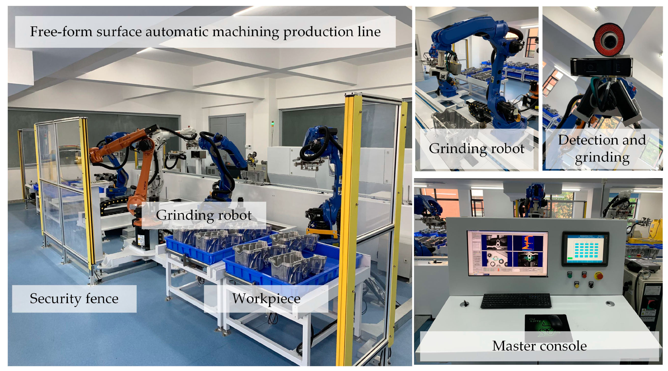
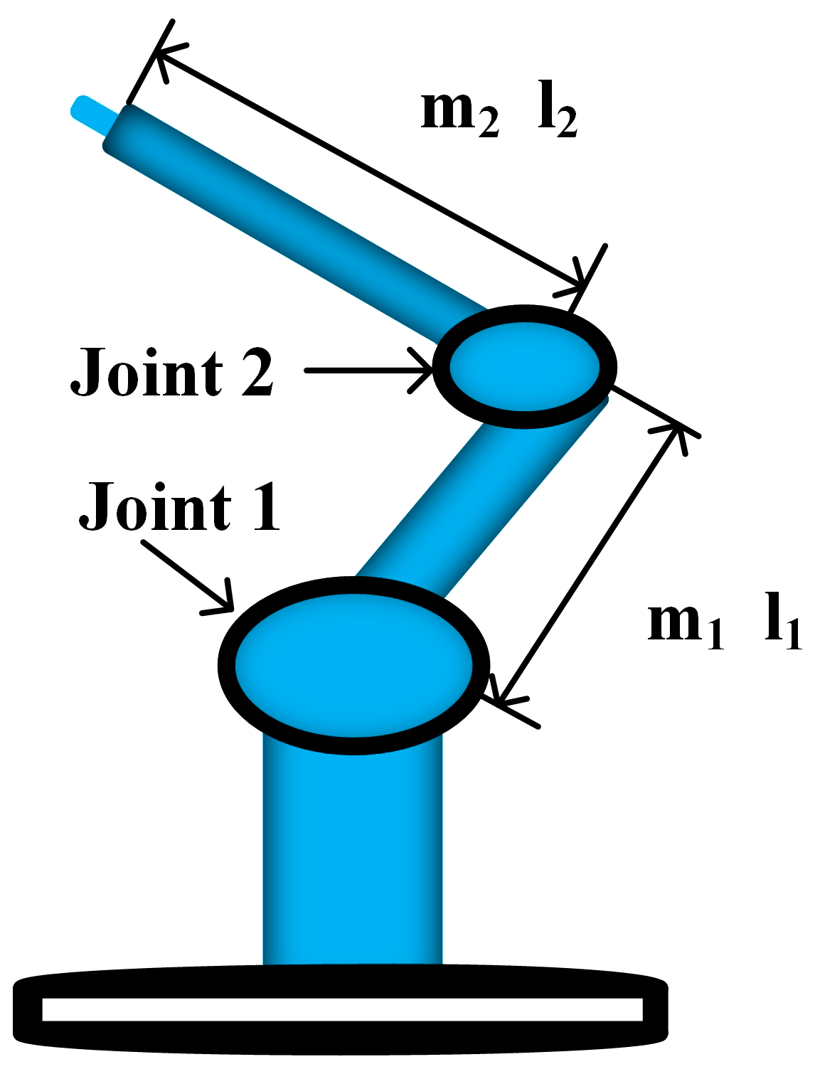
2.1. System Model of Free-Form Surface Grinding Robot

The dynamics of an FFSGR can be considered as the dynamics of an n-link robot manipulator, which are expressed as follows [41]:

$$M\left(q\right)\ddot{q}+C\left(q,\dot{q}\right)\dot{q}+G\left(q\right)+F\left(\dot{q}\right)+{\tau }_d=u_D$$

(1)

where $\left(q,\dot{q},\ddot{q}\right)\in R^{n\times 1}$ are the vectors of joint position, velocity, and acceleration, respectively. $M\left(q\right)\in R^{n\times n}$ is the nominal symmetric inertial matrix. $C\left(q,\dot{q}\right)\in R^{n\times n}$ are the vectors of the nominal Coriolis and centripetal forces, respectively. $G\left(q\right)\in R^{n\times 1}$ expresses the nominal gravity vector. $F\left(\dot{q}\right)\in R^{n\times 1}$ expresses the friction vector. ${\tau }_d\in R^{n\times 1}$ is the disturbance. $u_D\in R^{n\times 1}$ is the joint torque input vector with an actuator dead zone.

In practice, it is hard to establish the exact mathematical model of the FFSGR. Considering the model uncertainty, one gets:

$$\{\begin{array}{c}M\left(q\right)=M_0\left(q\right)+\Delta M\left(q\right)\\ C\left(q,\dot{q}\right)=C_0\left(q,\dot{q}\right)+\Delta C\left(q,\dot{q}\right)\\ G\left(q\right)=G_0\left(q\right)+\Delta G\left(q\right)\\ F\left(\dot{q}\right)=F_0\left(\dot{q}\right)+\Delta F\left(\dot{q}\right)\\ {\tau }_d={\tau }_0+\Delta \tau \end{array}.$$

(2)

The purpose is to design a torque controller $u_D$ for the FFSGR with an actuator dead zone to make the real trajectory track the desired one. To achieve this objective, three properties of the dynamics of the robot model (1) must be satisfied [41]:

Property 1.

$M\left(q\right)$is a positive definite symmetric matrix and uniformly bounded:

$$m_1{\Vert x\Vert }^2\le x^{T}M\left(q\right)x\le m_2{\Vert x\Vert }^2, \forall x\in R^{n\times 1}$$

where$m_1$and$m_2$ are known positive constants and they depend on the mass of the robot manipulators.

Property 2.

$\dot{M}\left(q\right)-2C\left(q,\dot{q}\right)$ is a skew symmetric matrix for any vector$x$:

$$x^T\left(\dot{M}\left(q\right)-2C\left(q,\dot{q}\right)\right)x=0$$

Property 3.

$C\left(q,\dot{q}\right)\dot{q}$,$G\left(q\right)$,$F\left(\dot{q}\right)$, and${\tau }_d$are bounded as follows:

$$\Vert C\left(q,\dot{q}\right)\dot{q}\Vert \le C_k{\Vert \dot{q}\Vert }^2, \Vert G\left(q\right)\Vert \le G_k, \Vert F\left(\dot{q}\right)\Vert \le F_k , \Vert {\tau }_d\Vert \le {\tau }_k ,$$

where$C_k$,$F_k$,$G_k$, and${\tau }_k$are positive constants.

Remark 1.

The abovementionedpropertiesare not very strict, and they are common assumptions in the literature about robot control [36].

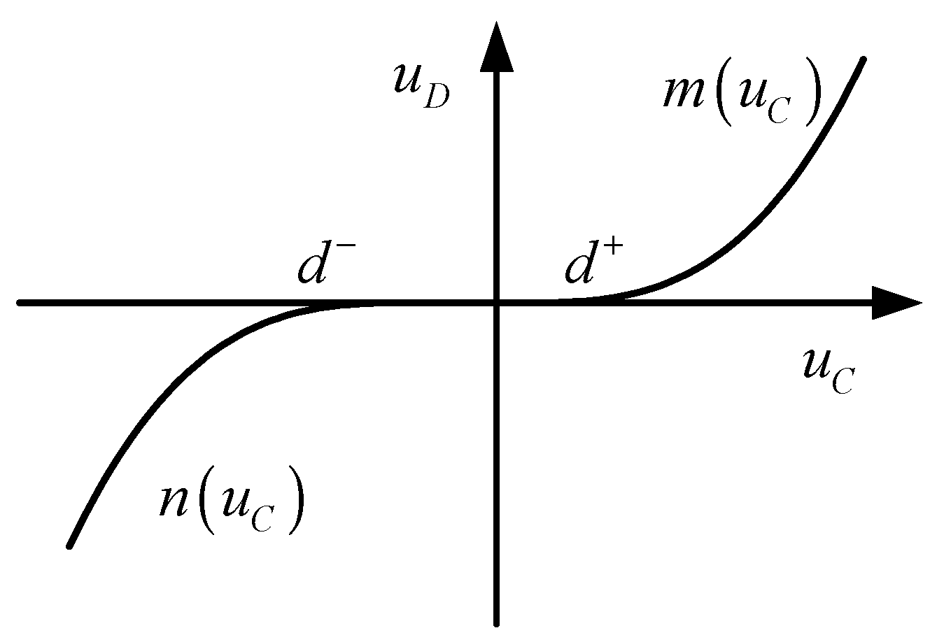
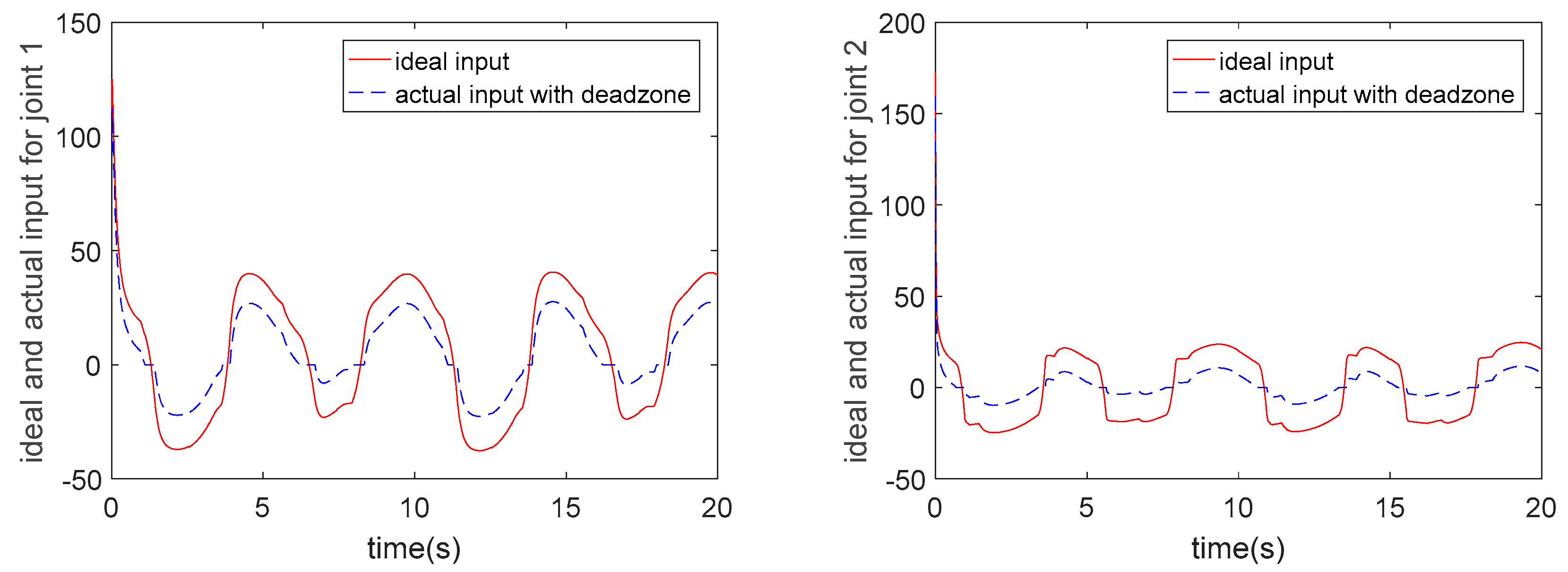
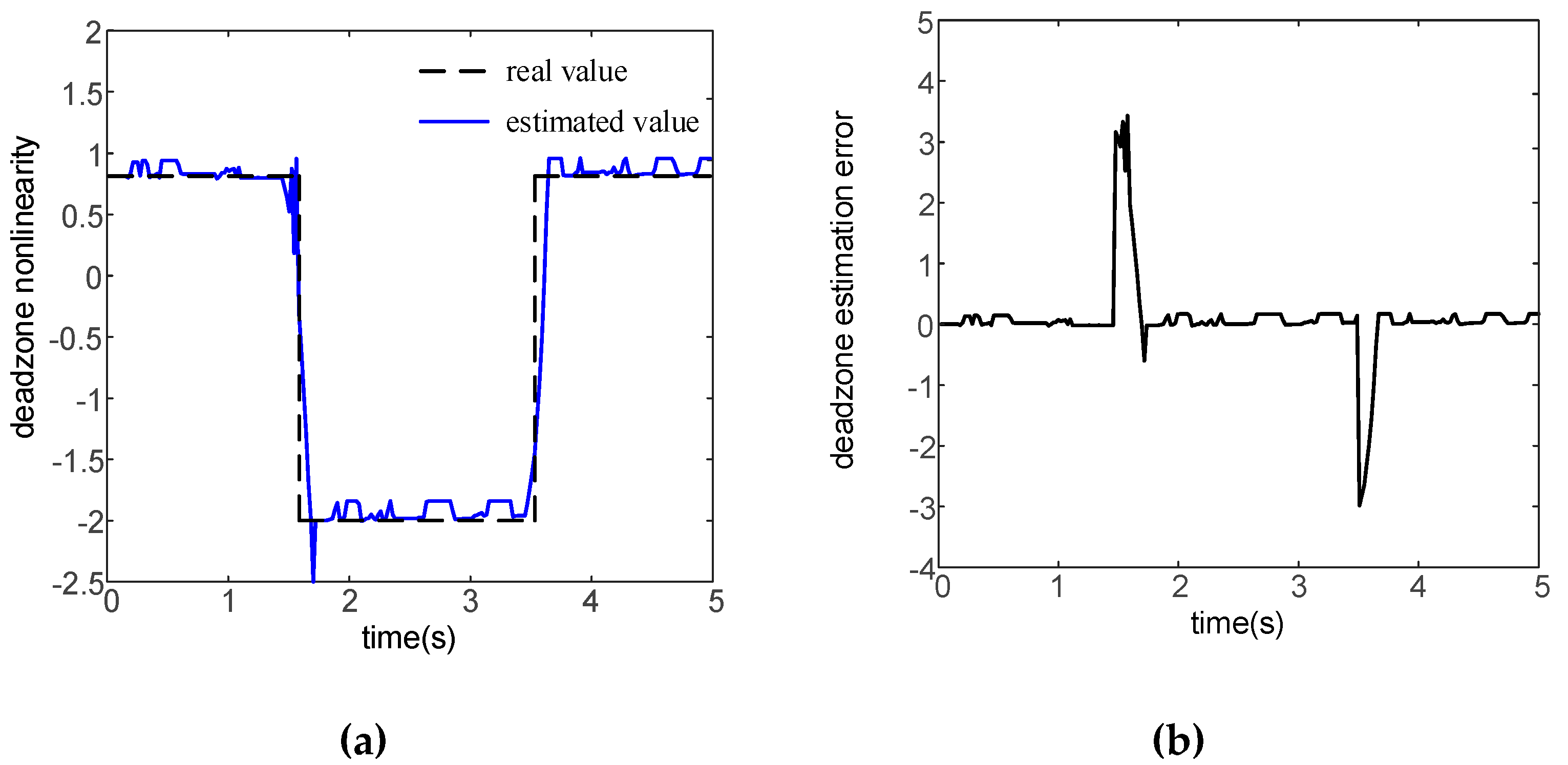
2.2. Dead Zone Non-Linearity Description

The dead zone is usually described as a static non-linear function that indicates the system’s insensitivity to small signals. For non-linear systems, the dead zone prevents the system from responding to some small signals and, finally, leads to significant tracking errors.

Generally, a dead zone’s non-symmetric non-linearity can be depicted as in Figure 2, and its mathematical model can be described as follows [10,36]:

$$u_D=D\left(u_C\right)=\{\begin{array}{cc}n\left(u_C\right)& u_C\le d^{-}\\ 0& d^{-}<u_C<d^{+}\\ m\left(u_C\right)& u_C\ge d^{+}\end{array} ,$$

(3)

where $u_C$ and $u_D$ denote the input signal and the dead zone output signal, respectively. $m\left(u_C\right)$ and $n\left(u_C\right)$ are smooth non-linear unknown functions. $d^{+}$ and $d^{-}$ are also unknown boundaries and represent most of the dead zone phenomena.

Assumption 1.

$m\left(u_C\right)$and$n\left(u_C\right)$ are all monotonically increasing, smooth, and invertible [10].

Then, the inverse of $D\left(u_C\right)$ can be obtained as:

$$D^{-1}\left(u\right)=\{\begin{array}{cc}{n}^{-1}\left(u\right)& u<0\\ 0& u=0\\ m^{-1}\left(u\right)& u>0\end{array}$$

(4)

and depicted as in Figure 3.

Thus, the following property is satisfied:

$$D\left(D^{-1}\left(u\right)\right)=u.$$

(5)

3. An Adaptive Robust Controller Using SMCs and RBFNNs

The proposed dead zone compensation scheme is shown in Figure 4. $O_1$ is used for dead zone compensation and $O_2$ is used for dead zone estimation. Where $u$ is the ideal control signal, $u_c$ and $u_d$ are unknown vectors and represent the input and the output of the dead zone, respectively [10].

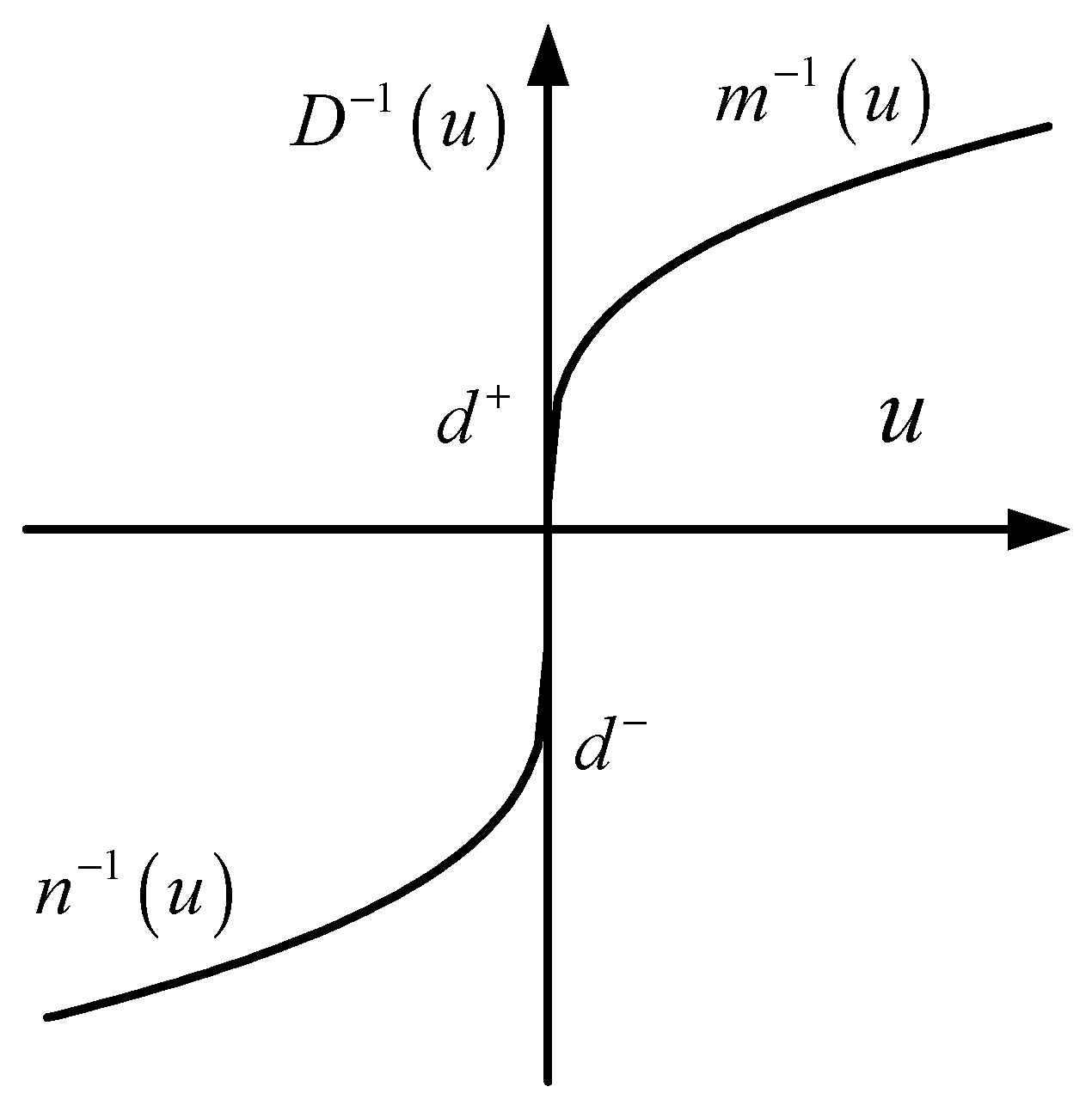
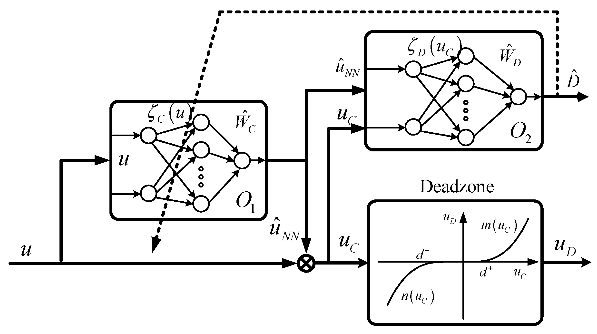
3.1. Dead Zone Compensation Algorithm

The dead zone inverse can be expressed in the equivalent form as [42]:

$$D^{-1}\left(u\right)=u+u_{NN}$$

(6)

From Equations (4) and (6), one can get $u_{NN}$ as follows:

$$u_{NN}=\{\begin{array}{cc}{m}^{-1}\left(u\right)-u& u_C<0\\ 0& u_C=0\\ n^{-1}\left(u\right)-u& u_C>0\end{array}$$

(7)

According to the approximation theory, the ideal output values of the dead zone estimation and compensation are calculated as:

$$\{\begin{array}{c}D\left(u_C\right)={\left\{W_D\right\}}^T\cdot {\zeta }_D\left(u_C\right)+{\delta }_D\left(u_C\right)\\ u_{NN}={\left\{W_C\right\}}^T\cdot {\zeta }_C\left(u\right)+{\delta }_C\left(u\right)\end{array}$$

(8)

where $W_D$ and $W_C$ are the values of the ideal weights, ${\zeta }_D\left(u_C\right)$ and ${\zeta }_C\left(u\right)$ are outputs of the hidden layer, and ${\delta }_D\left(u_C\right)$ and ${\delta }_C\left(u\right)$ are modeling errors.

The actual output can be given as follows:

$$\{\begin{array}{c}\widehat{D}\left(u_C\right)={\left\{{\widehat{W}}_D\right\}}^T\cdot \left\{{\zeta }_D\left(u_C\right)\right\}\\ {\widehat{u}}_{NN}={\left\{{\widehat{W}}_C\right\}}^T\cdot \left\{{\zeta }_C\left(u\right)\right\}\end{array}$$

(9)

where ${\widehat{W}}_D$ and ${\widehat{W}}_C$ are estimators of the weight values.

To define ${\tilde{W}}_D$ and ${\tilde{W}}_C$ as the error weights estimators:

$$\{\begin{array}{c}{\tilde{W}}_D=W_D-{\widehat{W}}_D\\ {\tilde{W}}_C=W_C-{\widehat{W}}_C\end{array}$$

(10)

The purpose of dead zone compensation is to generate an actual control signal with the dead zone $u_d$, tracking the ideal control law u. The relationship between $u$ and $u_D$ is given by

Theorem 1.

$$\begin{array}{ll}{u}_D=& u-{\left\{{\widehat{W}}_D\right\}}^T\cdot \left\{{\zeta }_D^{\prime }\left(u_c\right)\right\}\cdot {\left\{{\tilde{W}}_C\right\}}^T\cdot \left\{{\zeta }_C\left(u\right)\right\}+\\ & {\left\{{\tilde{W}}_D\right\}}^T\cdot \left\{{\zeta }_D^{\prime }\left(u_c\right)\right\}\cdot {\left\{{\widehat{W}}_C\right\}}^T\cdot \left\{{\zeta }_C\left(u\right)\right\}+d\end{array}$$

(11)

$d$is the modeling mismatch, represented as:

$$d=-{\left\{{\tilde{W}}_D\right\}}^T\cdot \left\{{\zeta }_D^{\prime }\left(u_c\right)\right\} \cdot {\left\{W_C\right\}}^T\cdot \left\{{\zeta }_C\left(u\right)\right\}-b+{\delta }_D\left(u_C\right)$$

(12)

Here,

$$b={\left\{W_D\right\}}^T\cdot \left\{\left({\zeta }_D^{\prime }\left(u+{\left\{{\widehat{W}}_C\right\}}^T\cdot \left\{{\zeta }_C\left(u\right)\right\}\right)\right)\cdot \left({\delta }_C\left(u\right)\right)\right\}+{\left\{W_D\right\}}^T\cdot \left\{R\left({\tilde{W}}_C,u\right)\right\}+{\delta }_D\left(u_C\right)$$

(13)

with$R\left({\widehat{W}}_C,u\right)$defined in the proof.

Proof. 

From Equations (3) and (8), the dead zone output of the FFSGR is:

$$\begin{array}{ll}{u}_D& =D\left(u_C\right)={\left\{W_D\right\}}^T\cdot {\zeta }_D\left(u_C\right)+{\delta }_D\left(u_C\right)\\ & ={\left\{W_D\right\}}^T\cdot {\zeta }_D\left(u+{\widehat{u}}_{NN}\left(u\right)\right)+{\delta }_D\left(u+{\widehat{u}}_{NN}\left(u\right)\right)\end{array}$$

(14)

and from Equations (5) and (6), one has:

$$u=D\left(D^{-1}\left(u\right)\right)=D\left(u+u_{NN}\left(u\right)\right)$$

(15)

Substituting Equation (8) into (15):

$$\begin{array}{ll}u& ={\left\{W_D\right\}}^T\cdot {\zeta }_D\left(u+u_{NN}\left(u\right)\right)+{\delta }_D\left(u+u_{NN}\left(u\right)\right)\\ & ={\left\{W_D\right\}}^T\cdot {\zeta }_D\left(u+{\left\{W_C\right\}}^T\cdot {\zeta }_C\left(u\right)+{\delta }_C\left(u\right)\right)+{\delta }_D\left(u+u_{NN}\left(u\right)\right)\\ & ={\left\{W_D\right\}}^T\cdot {\zeta }_D\left(u+{\left\{{\widehat{W}}_C\right\}}^T\cdot {\zeta }_C\left(u\right)+{\left\{{\tilde{W}}_C\right\}}^T\cdot {\zeta }_C\left(u\right)+{\delta }_C\left(u\right)\right)+{\delta }_D\left(u+u_{NN}\left(u\right)\right)\end{array}$$

(16)

Let $x=u+{\left\{{\widehat{W}}_C\right\}}^T\cdot {\zeta }_C\left(u\right)+{\left\{{\tilde{W}}_C\right\}}^T\cdot {\zeta }_C\left(u\right)+{\delta }_C\left(u\right)$, $x_0=u+{\left\{{\widehat{W}}_C\right\}}^T\cdot {\zeta }_C\left(u\right)$ Then, $x-x_0={\left\{{\tilde{W}}_C\right\}}^T\cdot {\zeta }_C\left(u\right)+{\delta }_C\left(u\right)$.

Let $f\left(x\right)={\zeta }_D\left(x\right)$, using the Taylor series expansion $f\left(x\right)=f\left(x_0\right)+f^{\prime }\left(x_0\right)\left(x-x_0\right)+R\left(\xi \right)$; where $R\left(\xi \right)=1/2!{\zeta }_D^{"}\left({\xi }_0\right){\left(x-x_0\right)}^2$, one has:

$$R\left(\xi \right)=R\left({\tilde{W}}_C,u\right)=\frac{1}{2!}{\zeta }_D^{"}\left({\xi }_0\right){\left({\left\{{\tilde{W}}_C\right\}}^T\cdot {\zeta }_C\left(u\right)+{\delta }_C\left(u\right)\right)}^2$$

(17)

then Equation (16) becomes

$$\begin{array}{ll}u=& {\left\{W_D\right\}}^T\cdot \left({\zeta }_D\left(x_0\right)+{\zeta }_D^{\prime }\left(x_0\right)\left(x-x_0\right)+R\left(\xi \right)\right)+{\delta }_D\left(u+u_{NN}\left(u\right)\right)\\ & ={\left\{W_D\right\}}^T\cdot {\zeta }_D\left(u+{\left\{{\widehat{W}}_C\right\}}^T\cdot {\zeta }_C\left(u\right)\right)+\\ & {\left\{W_D\right\}}^T\cdot {\zeta }_D^{\prime }\left(u+{\left\{{\widehat{W}}_C\right\}}^T\cdot {\zeta }_C\left(u\right)\right)\cdot \left({\left\{{\tilde{W}}_C\right\}}^T\cdot {\zeta }_C\left(u\right)+{\delta }_C\left(u\right)\right)+\\ & {\left\{W_D\right\}}^T\cdot R\left(\xi \right)+{\delta }_D\left(u+u_{NN}\left(u\right)\right)\end{array}$$

(18)

Substituting $b$ given by Equation (13) into (18), one has:

$$\begin{array}{ll}u=& {\left\{W_D\right\}}^T\cdot {\zeta }_D\left(u+{\left\{{\widehat{W}}_C\right\}}^T\cdot {\zeta }_C\left(u\right)\right)+\\ & {\left\{W_D\right\}}^T\cdot {\zeta }_D^{\prime }\left(u+{\left\{{\widehat{W}}_C\right\}}^T\cdot {\zeta }_C\left(u\right)\right)\cdot {\left\{{\tilde{W}}_C\right\}}^T\cdot {\zeta }_C\left(u\right)+b\end{array}$$

(19)

Combining Equations (9) and (19), one has:

$$\begin{array}{lll}u+{\delta }_D\left(u_C\right)\hfill & =\hfill & {\left\{W_D\right\}}^T\cdot {\zeta }_D\left(u+{\left\{{\widehat{W}}_C\right\}}^T\cdot {\zeta }_C\left(u\right)\right)+\hfill \\ \hfill & \hfill & {\left\{{\widehat{W}}_D\right\}}^T\cdot {\zeta }_D^{\text{'}}\left(u+{\left\{{\widehat{W}}_C\right\}}^T\cdot {\zeta }_C\left(u\right)\right)\cdot {\left\{{\tilde{W}}_C\right\}}^T\cdot {\zeta }_C\left(u\right)+\hfill \\ \hfill & \hfill & {\left\{{\tilde{W}}_D\right\}}^T\cdot {\zeta }_D^{\text{'}}\left(u+{\left\{{\widehat{W}}_C\right\}}^T\cdot {\zeta }_C\left(u\right)\right)\cdot {\left\{{\tilde{W}}_C\right\}}^T\cdot {\zeta }_C\left(u\right)+b+{\delta }_D\left(u_C\right)\hfill \\ \hfill & =\hfill & {\left\{W_D\right\}}^T\cdot {\zeta }_D\left(u_C\right)+{\left\{{\widehat{W}}_D\right\}}^T\cdot {\zeta }_D^{\text{'}}\left(u_C\right)\cdot {\left\{{\tilde{W}}_C\right\}}^T\cdot {\zeta }_C\left(u\right)+\hfill \\ \hfill & \hfill & {\left\{{\tilde{W}}_D\right\}}^T\cdot {\zeta }_D^{\text{'}}\left(u_C\right)\cdot {\left\{{\tilde{W}}_C\right\}}^T\cdot {\zeta }_C\left(u\right)+b+{\delta }_D\left(u_C\right)\hfill \\ \hfill & =\hfill & {\left\{W_D\right\}}^T\cdot {\zeta }_D\left(u_C\right)+{\left\{{\widehat{W}}_D\right\}}^T\cdot {\zeta }_D^{\text{'}}\left(u_C\right)\cdot {\left\{{\tilde{W}}_C\right\}}^T\cdot {\zeta }_C\left(u\right)+\hfill \\ \hfill & \hfill & {\left\{{\tilde{W}}_D\right\}}^T\cdot {\zeta }_D^{\text{'}}\left(u_C\right)\cdot {\left\{W_C\right\}}^T\cdot {\zeta }_C\left(u\right)-{\left\{{\tilde{W}}_D\right\}}^T\cdot {\zeta }_D^{\text{'}}\left(u_C\right)\cdot {\left\{{\widehat{W}}_C\right\}}^T\cdot {\zeta }_C\left(u\right)+b+{\delta }_D\left(u_C\right)\hfill \end{array}$$

(20)

Combining Equations (12), (14), and (20), one gets:

$$\begin{array}{ll}{u}_D=& u-{\left\{{\widehat{W}}_D\right\}}^T\cdot \left\{{\zeta }_D^{\prime }\left(u_C\right)\right\}\cdot {\left\{{\tilde{W}}_C\right\}}^T\cdot \left\{{\zeta }_C\left(u\right)\right\}+\\ & {\left\{{\tilde{W}}_D\right\}}^T\cdot \left\{{\zeta }_D^{\prime }\left(u_C\right)\right\}\cdot {\left\{{\widehat{W}}_C\right\}}^T\cdot \left\{{\zeta }_C\left(u\right)\right\}+d\end{array}$$

(21)

□

Theorem 2.

The norm of modeling mismatch$d$is bounded, and the upper bound is as follows:

$$\Vert d\Vert \le i_1{\Vert {\tilde{W}}_D\Vert }_F+i_2{\Vert {\tilde{W}}_C\Vert }_F^2+i_3{\Vert {\tilde{W}}_C\Vert }_F+i_4$$

(22)

where${\Vert {\tilde{W}}_D\Vert }_F$,${\Vert {\tilde{W}}_C\Vert }_F$are the Frobenius norm of${\tilde{W}}_D$,${\tilde{W}}_C$. $i_2$,$i_3$, and$i_4$are constants and can be calculated.

Proof. 

From the definition of $d$ in (12), one has:

$$\begin{array}{l}\Vert d\Vert \le {\Vert {\tilde{W}}_D\Vert }_F\cdot \Vert {\zeta }_D^{\prime }\left(u_C\right)\Vert \cdot {\Vert W_C\Vert }_F\cdot \Vert {\zeta }_C\left(u\right)\Vert +\Vert b\left(t\right)\Vert +\Vert {\delta }_D\left(u_D\right)\Vert \\ \le {\Vert {\tilde{W}}_D\Vert }_F\cdot \Vert {\zeta }_D^{\prime }\left(u_C\right)\Vert \cdot \Vert W_{CM}\Vert \cdot \Vert {\zeta }_C\left(u\right)\Vert +\Vert b\Vert +{\delta }_N\\ =i_1{\Vert {\tilde{W}}_D\Vert }_F+\Vert b\Vert +{\delta }_N\end{array}$$

(23)

where $i_1=\Vert {\zeta }_D^{\prime }\left(u_c\right)\Vert \cdot \Vert W_{CM}\Vert \cdot \Vert {\zeta }_C\left(u\right)\Vert$, ${\delta }_N=\Vert {\delta }_D\left(u_C\right)\Vert$, $\Vert W_{CM}\Vert$ is the maximum value of ${\Vert W_C\Vert }_F$.

From the definition of $b$ in Equation (13) and the Taylor expansion remainder in Equation (17), one has:

$$\begin{array}{lll}\Vert b\Vert \hfill & \le \hfill & {\Vert W_D\Vert }_F\cdot \Vert {\zeta }_D^{\text{'}}\left(u_C\right)\Vert \cdot \Vert {\delta }_C\left(u\right)\Vert +\frac{1}{2}{\Vert W_D\Vert }_F\cdot \Vert {\zeta }_D^{"}\left({\xi }_0\right)\Vert \cdot {\Vert {\tilde{W}}_C\Vert }_F^2\cdot {\Vert {\zeta }_C\left(u\right)\Vert }^2+\hfill \\ \hfill & \hfill & {\Vert W_D\Vert }_F\cdot \Vert {\zeta }_D^{"}\left({\xi }_0\right)\Vert \cdot {\Vert {\tilde{W}}_C\Vert }_F\cdot \Vert {\zeta }_C\left(u\right)\Vert \cdot \Vert {\delta }_C\left(u\right)\Vert +\hfill \\ \hfill & \hfill & \frac{1}{2}{\Vert W_D\Vert }_F\cdot \Vert {\zeta }_D^{"}\left({\xi }_0\right)\Vert \cdot {\Vert {\delta }_C\left(u\right)\Vert }^2+\Vert {\delta }_D\left(u_C\right)\Vert \hfill \\ \hfill & \le \hfill & W_{DM}\cdot \Vert {\zeta }_D^{\text{'}}\left(u_C\right)\Vert \cdot {\delta }_{CN}+\frac{1}{2}{W}_{DM}\cdot \Vert {\zeta }_D^{"}\left({\xi }_0\right)\Vert \cdot {\Vert {\tilde{W}}_C\Vert }_F^2\cdot {\Vert {\zeta }_C\left(u\right)\Vert }^2+\hfill \\ \hfill & \hfill & W_{DM}\cdot \Vert {\zeta }_D^{"}\left({\xi }_0\right)\Vert \cdot {\Vert {\tilde{W}}_C\Vert }_F\cdot \Vert {\zeta }_C\left(u\right)\Vert \cdot {\delta }_{CN}+\frac{1}{2}{W}_{DM}\cdot \Vert {\zeta }_D^{"}\left({\xi }_0\right)\Vert \cdot {\delta }_{CN}^2+{\delta }_{DN}\hfill \\ \hfill & \hfill & =i_2{\Vert {\tilde{W}}_C\Vert }_F^2+i_3{\Vert {\tilde{W}}_C\Vert }_F+i_4\hfill \end{array}$$

(24)

where $W_{DM}$, ${\delta }_{DN}$, and ${\delta }_{CN}$ is the maximum of ${\Vert W_D\Vert }_F$, $\Vert {\delta }_D\left(u_D\right)\Vert$ and $\Vert {\delta }_C\left(u\right)\Vert$, respectively. Moreover, $i_2=0.5W_{DM}\cdot \Vert {\zeta }_D^{"}\left({\xi }_0\right)\Vert \cdot {\Vert {\zeta }_C\left(u\right)\Vert }^2$, $i_3= W_{DM}\cdot \Vert {\zeta }_D^{"}\left({\xi }_0\right)\Vert \cdot \Vert {\zeta }_C\left(u\right)\Vert \cdot {\delta }_{CN}$, and $i_4= W_{DM}\cdot \Vert {\zeta }_D^{\prime }\left(u_C\right)\Vert \cdot {\delta }_{CN}+0.5W_{DM}\cdot \Vert {\zeta }_D^{"}\left({\xi }_0\right)\Vert \cdot {\delta }_{CN}^2+{\delta }_{DN}$.

Theorem 2 is proven by Equations (23) and (24). From Theorem 2, one can get the upper bound of the $d\left(t\right)$ in Equation (12), which ensures the stability of the system.

The adaptive machine learning law of RBFNNs can be designed as:

$$\{\begin{array}{c}{\dot{\widehat{W}}}_D=-S\cdot {\zeta }_D^{\prime }\left(u_C\right)\cdot {\left\{{\widehat{W}}_C\right\}}^T\cdot {\zeta }_C\left(u\right)\cdot s-K_1\cdot S\cdot \Vert s\Vert \cdot {\widehat{W}}_D\\ {\dot{\widehat{W}}}_C=T\cdot {\zeta }_C\left(u\right)\cdot s\cdot {\widehat{W}}_D\cdot {\zeta }_D^{\prime }\left(u_C\right)-K_1\cdot T\cdot \Vert s\Vert \cdot {\widehat{W}}_C-K_2\cdot T\cdot \Vert s\Vert \cdot {\Vert {\widehat{W}}_C\Vert }_F\cdot {\widehat{W}}_C\end{array}$$

(25)

where ${\widehat{W}}_C$ and ${\widehat{W}}_D$ are the weight value vector of $O_1$ and $O_2$, respectively, as illustrated in Figure 4. $S=S^T$, $T=T^T$ are positive constant symmetric matrices, and $K_1>0$, $K_2>0$. □

3.2. Controller Design and Stability Analysis

In this study, the proposed dead-zone compensation-based adaptive control method was applied to improve the trajectory tracking performance of the FFSGR, with the actuator dead zone for non-linearity.

The adaptive tracking control scheme is shown in Figure 5 and mainly consisted of two parts. The first part was the ideal controller, and the second part was the dead zone estimation and compensation:

$$u_C=u+{\widehat{u}}_{NN}\left(u\right)$$

(26)

where ${\widehat{u}}_{NN}\left(u\right)$ is the compensation item for the dead zone introduced in Section 3. $u$ is the ideal control signal and the design is shown in the following section.

The trajectory tracking error was defined as:

$$e\left(t\right)=q_d\left(t\right)-q\left(t\right)$$

(27)

Compared to other sliding surfaces, the parameter design of the linear sliding surface was simpler and can be more easily implemented in engineering, since only the slope of the sliding surface should be designed. Therefore, the sliding surface is introduced here and designed as follows:

$$s\left(t\right)=ce\left(t\right)+\dot{e}\left(t\right)$$

(28)

where c is the gain matrix of the sliding mode’s surface.

Defining the auxiliary error variable $q_s\left(t\right)={\displaystyle \int s\left(t\right)dt}+q\left(t\right)$, from Equations (27) and (28), one obtains the derivatives:

$$\{\begin{array}{c}{\dot{q}}_s=s\left(t\right)+\dot{q}\left(t\right)\\ {\ddot{q}}_s=c\dot{e}\left(t\right)+{\ddot{q}}_d\left(t\right)\end{array}$$

(29)

Combining Equations (1) and (29) yields:

$$\begin{array}{l}M\left(q\right)\dot{s}\left(t\right)=M\left(q\right){\ddot{q}}_s-M\left(q\right)\ddot{q}\\ \hspace{1em}\hspace{1em}\hspace{1em}\hspace{1em}=M\left(q\right){\ddot{q}}_s+C\left(q,\dot{q}\right)\dot{q}+G\left(q\right)+F\left(\dot{q}\right)+{\tau }_d-u_D\\ \hspace{1em}\hspace{1em}\hspace{1em}\hspace{1em}=M\left(q\right){\ddot{q}}_s+C\left(q,\dot{q}\right)\left({\dot{q}}_s-s\left(t\right)\right)+G\left(q\right)+F\left(\dot{q}\right)+{\tau }_d-u_D\\ \hspace{1em}\hspace{1em}\hspace{1em}\hspace{1em}=-C\left(q,\dot{q}\right)s\left(t\right)+f-u_D\end{array}$$

(30)

where $f=M\left(q\right){\ddot{q}}_s+C\left(q,\dot{q}\right){\dot{q}}_s+G\left(q\right)+F\left(\dot{q}\right)+{\tau }_d$, which represents the system dynamics.

The ideal adaptive robust control law using RBFNNs and a sliding mode is:

$$u=f_0+K_{g}s\left(t\right)-K_s\mathrm{sgn}\left(s\left(t\right)\right)$$

(31)

where $f_0=M_0\left(q\right){\ddot{q}}_s+C_0\left(q,\dot{q}\right){\dot{q}}_s+G_0\left(q\right)+F_0\left(\dot{q}\right)+{\tau }_0$, and the modeling error is

$$\begin{array}{l}\tilde{f}=f-f_0\\ =\Delta M\left(q\right){\ddot{q}}_s+\Delta C\left(q,\dot{q}\right){\dot{q}}_s+\Delta G\left(q\right)+\Delta F\left(\dot{q}\right)+\Delta {\tau }_d\end{array}$$

(32)

$\Vert \tilde{f}\Vert \le f_M$, $f_M$ is the maximum value of $\tilde{f}$. $K_g>0$ and $K_s>0$ are often chosen as diagonal matrices. Substituting ideal control law (31) and the relationship with dead zone output Equations (11) into (30) yields the closed loop error dynamics:

$$\begin{array}{ll}M\left(q\right)\dot{s}\left(t\right)=& -C\left(q,\dot{q}\right)s\left(t\right)-K_{g}s\left(t\right)+{\left\{{\widehat{W}}_D\right\}}^T\cdot \left\{{\zeta }_D^{\prime }\left(u_c\right)\right\}\cdot {\left\{{\tilde{W}}_C\right\}}^T\cdot \left\{{\zeta }_C\left(u\right)\right\}-\\ & {\left\{{\tilde{W}}_D\right\}}^T\cdot \left\{{\zeta }_D^{\prime }\left(u_c\right)\right\}\cdot {\left\{{\widehat{W}}_C\right\}}^T\cdot \left\{{\zeta }_C\left(u\right)\right\}+\tilde{f}-d-K_s\mathrm{sgn}\left(s\left(t\right)\right)\end{array}$$

(33)

Theorem 3.

Given the system in (1), selecting the tracking control law (31) plus the dead zone estimation and compensation law (9) as well as the adaptive tuning law (25), the closed loop error of the control system is uniformly bounded. Moreover, the tracking error can be kept as small as desired by increasing the gain$K_g$.

Proof. 

To guarantee the stability of the total control system, the Lyapunov function was chosen as follows:

$$V=\frac{1}{2}{s}^T\left(t\right)M\left(q\right)s\left(t\right)+\frac{1}{2}{\displaystyle \sum _{k=1}^n{\left\{{\tilde{W}}_{Dk}\right\}}^T{S}^{-1}\left\{{\tilde{W}}_{Dk}\right\}}+\frac{1}{2}{\displaystyle \sum _{k=1}^n{\left\{{\tilde{W}}_{Ck}\right\}}^T{T}^{-1}\left\{{\tilde{W}}_{Ck}\right\}}$$

(34)

and the derivative was:

$$\dot{V}=s^T\left(t\right)\left(M\left(q\right)\dot{s}\left(t\right)+C\left(q,\dot{q}\right)s\left(t\right)\right)+{\displaystyle \sum _{k=1}^n{\left\{{\tilde{W}}_{Dk}\right\}}^T{S}^{-1}\left\{{\dot{\tilde{W}}}_{Dk}\right\}}+{\displaystyle \sum _{k=1}^n{\left\{{\tilde{W}}_{Ck}\right\}}^T{T}^{-1}\left\{{\dot{\tilde{W}}}_{Ck}\right\}}$$

(35)

Substituting Equations (33) into (35), one gets:

$$\begin{array}{lll}\dot{V}\hfill & =\hfill & s^T\left(t\right)\left(\begin{array}{l}-K_{g}s\left(t\right)+{\left\{{\widehat{W}}_D\right\}}^T\cdot \left\{{\zeta }_D^{\text{'}}\left(u_c\right)\right\}\cdot {\left\{{\tilde{W}}_C\right\}}^T\cdot \left\{{\zeta }_C\left(u\right)\right\}-\\ {\left\{{\tilde{W}}_D\right\}}^T\cdot \left\{{\zeta }_D^{\text{'}}\left(u_c\right)\right\}\cdot {\left\{{\widehat{W}}_C\right\}}^T\cdot \left\{{\zeta }_C\left(u\right)\right\}+\\ \tilde{f}-d-K_s\mathrm{sgn}\left(s\left(t\right)\right)\end{array}\right)+\hfill \\ \hfill & \hfill & {\displaystyle \sum _{k=1}^n{\left\{{\tilde{W}}_{Dk}\right\}}^T{S}^{-1}\left\{{\dot{\tilde{W}}}_{Dk}\right\}}+{\displaystyle \sum _{k=1}^n{\left\{{\tilde{W}}_{Ck}\right\}}^T{T}^{-1}\left\{{\dot{\tilde{W}}}_{Ck}\right\}} \hfill \\ \hfill & =\hfill & -s^T\left(t\right)K_{g}s\left(t\right)+s^T\left(t\right){\left\{{\widehat{W}}_D\right\}}^T\cdot \left\{{\zeta }_D^{\text{'}}\left(u_c\right)\right\}\cdot {\left\{{\tilde{W}}_C\right\}}^T\cdot \left\{{\zeta }_C\left(u\right)\right\}-\hfill \\ \hfill & \hfill & s^T\left(t\right){\left\{{\tilde{W}}_D\right\}}^T\cdot \left\{{\zeta }_D^{\text{'}}\left(u_c\right)\right\}\cdot {\left\{{\widehat{W}}_C\right\}}^T\cdot \left\{{\zeta }_C\left(u\right)\right\}+\hfill \\ \hfill & \hfill & s^T\left(t\right)\tilde{f}-s^T\left(t\right)d-s^T\left(t\right)K_s\mathrm{sgn}\left(s\left(t\right)\right)+\hfill \\ \hfill & \hfill & {\displaystyle \sum _{k=1}^n{\left\{{\tilde{W}}_{Dk}\right\}}^T{S}^{-1}\left\{{\dot{\tilde{W}}}_{Dk}\right\}}+{\displaystyle \sum _{k=1}^n{\left\{{\tilde{W}}_{Ck}\right\}}^T{T}^{-1}\left\{{\dot{\tilde{W}}}_{Ck}\right\}}\hfill \end{array}$$

(36)

Combining adaptive law (25) with (36):

$$\begin{array}{lll}\dot{V}\hfill & =\hfill & -s^T\left(t\right)K_{g}s\left(t\right)+s^T\left(t\right){\left\{{\widehat{W}}_D\right\}}^T\cdot \left\{{\zeta }_D^{\text{'}}\left(u_c\right)\right\}\cdot {\left\{{\tilde{W}}_C\right\}}^T\cdot \left\{{\zeta }_C\left(u\right)\right\}-\hfill \\ \hfill & \hfill & s^T\left(t\right){\left\{{\tilde{W}}_D\right\}}^T\cdot \left\{{\zeta }_D^{\text{'}}\left(u_c\right)\right\}\cdot {\left\{{\widehat{W}}_C\right\}}^T\cdot \left\{{\zeta }_C\left(u\right)\right\}+\hfill \\ \hfill & \hfill & s^T\left(t\right)\tilde{f}-s^T\left(t\right)d-s^T\left(t\right)K_s\mathrm{sgn}\left(s\left(t\right)\right)+\hfill \\ \hfill & \hfill & {\displaystyle \sum _{k=1}^n{\left\{{\tilde{W}}_{Dk}\right\}}^T\left({\zeta }_D^{\text{'}}\left(u_{Ck}\right)\cdot {\left\{{\widehat{W}}_{Ck}\right\}}^T\cdot {\zeta }_C\left(u_k\right)\cdot s_k+K_1\cdot \Vert s_k\Vert \cdot {\widehat{W}}_{Dk}\right)+}\hfill \\ \hfill & \hfill & {\displaystyle \sum _{k=1}^n{\left\{{\tilde{W}}_{Ck}\right\}}^T}\left(-{\zeta }_C\left(u_k\right)\cdot s_k\cdot {\widehat{W}}_{Dk}\cdot {\zeta }_D^{\text{'}}\left(u_{Ck}\right)+K_1\cdot \Vert s_k\Vert \cdot {\widehat{W}}_{Ck}+K_2\cdot \Vert s_k\Vert \cdot {\Vert {\widehat{W}}_C\Vert }_F\cdot {\widehat{W}}_{Ck} \right)\hfill \end{array}$$

(37)

Since

$$\{\begin{array}{c}{s}^T\left(t\right){\left\{{\tilde{W}}_D\right\}}^T\cdot \left\{{\zeta }_D^{\prime }\left(u_c\right)\right\}\cdot {\left\{{\widehat{W}}_C\right\}}^T\cdot \left\{{\zeta }_C\left(u\right)\right\}={\displaystyle \sum _{k=1}^n{\left\{{\tilde{W}}_{Dk}\right\}}^T\cdot \left\{{\zeta }_{Dk}^{\prime }\left(u_c\right)\right\}\cdot {\left\{{\widehat{W}}_{Ck}\right\}}^T\cdot \left\{{\zeta }_{Ck}\left(u\right)\right\}} s_k\left(t\right)\\ s^T\left(t\right){\left\{{\widehat{W}}_D\right\}}^T\cdot \left\{{\zeta }_D^{\prime }\left(u_c\right)\right\}\cdot {\left\{{\tilde{W}}_C\right\}}^T\cdot \left\{{\zeta }_C\left(u\right)\right\}={\displaystyle \sum _{k=1}^n{\left\{{\tilde{W}}_{Ck}\right\}}^T\cdot {\zeta }_{Ck}\left(u\right)\cdot {\left\{{\widehat{W}}_{Dk}\right\}}^T\cdot \left\{{\zeta }_{Dk}^{\prime }\left(u_C\right)\right\}} \end{array}$$

(38)

then.

$$\begin{array}{lll}\dot{V}\hfill & =\hfill & -s^T\left(t\right)K_{g}s\left(t\right)+ {\displaystyle \sum _{k=1}^n{\left\{{\tilde{W}}_{Dk}\right\}}^T{K}_1\Vert s\Vert {\widehat{W}}_{Dk}+}{\displaystyle \sum _{k=1}^n{\left\{{\tilde{W}}_{Ck}\right\}}^T\left(K_1\Vert s\Vert {\widehat{W}}_{Ck}+K_2\Vert s\Vert {\Vert {\widehat{W}}_C\Vert }_F{\widehat{W}}_{Ck}\right)}+\hfill \\ \hfill & \hfill & s^T\left(t\right)\tilde{f}-s^T\left(t\right)d-s^T\left(t\right)K_s\mathrm{sgn}\left(s\left(t\right)\right)\hfill \\ \hfill & =\hfill & -s^T\left(t\right)K_{g}s\left(t\right)+K_1\Vert s\Vert tr\left({\tilde{W}}_D^T{\widehat{W}}_D\right)+\Vert s\Vert tr\left({\tilde{W}}_C^T{K}_1{\widehat{W}}_C+{\tilde{W}}_C^T{K}_2{\Vert {\widehat{W}}_C\Vert }_F{\widehat{W}}_C\right)-\hfill \\ \hfill & \hfill & -s^T\left(t\right)d+ s^T\left(t\right)\left(\tilde{f}-K_s\mathrm{sgn}\left(s\left(t\right)\right)\right)\hfill \\ \hfill & =\hfill & -s^T\left(t\right)K_{g}s\left(t\right)+K_1\Vert s\Vert tr\left({\tilde{W}}_D^T\left(W_D-{\tilde{W}}_D\right)\right)-s^T\left(t\right)d+ s^T\left(t\right)\left(\tilde{f}-K_s\mathrm{sgn}\left(s\left(t\right)\right)\right)+\hfill \\ \hfill & \hfill & \Vert s\Vert tr\left({\tilde{W}}_C^T{K}_1\left(W_C-{\tilde{W}}_C\right)\right)+\Vert s\Vert tr\left({\tilde{W}}_C^T{K}_2{\Vert {\widehat{W}}_C\Vert }_F\left(W_C-{\tilde{W}}_C\right)\right)\hfill \end{array}$$

(39)

According to the inequality $\mathrm{tr}\left(\tilde{x}\left(x-\tilde{x}\right)\right)\le {\Vert \tilde{x}\Vert }_F{\Vert x\Vert }_F-{\Vert \tilde{x}\Vert }_F^2$, one has:

$$\{\begin{array}{c}tr\left({\tilde{W}}_D^T\left(W_D-{\tilde{W}}_D\right)\right)\le {\Vert {\tilde{W}}_D\Vert }_F{\Vert W_D\Vert }_F-{\Vert {\tilde{W}}_D\Vert }_F^2\le {\Vert {\tilde{W}}_D\Vert }_F\left(W_{DM}-{\Vert {\tilde{W}}_D\Vert }_F\right)\\ tr\left({\tilde{W}}_C^T{K}_1\left(W_C-{\tilde{W}}_C\right)\right)\le K_1\left({\Vert {\tilde{W}}_C\Vert }_F{\Vert W_C\Vert }_F-{\Vert {\tilde{W}}_C\Vert }_F^2\right)\le K_1{\Vert {\tilde{W}}_C\Vert }_F\left(W_{CM}-{\Vert {\tilde{W}}_C\Vert }_F\right)\\ tr\left({\tilde{W}}_C^T{K}_2{\Vert {\widehat{W}}_C\Vert }_F\left(W_C-{\tilde{W}}_C\right)\right)\le K_2{\Vert {\tilde{W}}_C\Vert }_F{W}_{CM}^2+2K_2{\Vert {\tilde{W}}_C\Vert }_F^2{W}_{CM}-K_2{\Vert {\tilde{W}}_C\Vert }_F^3\end{array}$$

(40)

According to Theorem 2, combining Equations (40) and (39):

$$\begin{array}{llll}\dot{V}\hfill & \le \hfill & -\Vert s\Vert \hfill & \left\{\begin{array}{l}{K}_{g\min }\Vert s\Vert -K_2{\Vert {\tilde{W}}_C\Vert }_F{W}_{CM}^2-2K_2{\Vert {\tilde{W}}_C\Vert }_F^2{W}_{CM}+K_2{\Vert {\tilde{W}}_C\Vert }_F^3-K_1{\Vert {\tilde{W}}_D\Vert }_F\left(W_{DM}-{\Vert {\tilde{W}}_D\Vert }_F\right)+\hfill \\ -K_1{\Vert {\tilde{W}}_C\Vert }_F\left(W_{CM}-{\Vert {\tilde{W}}_C\Vert }_F\right)-i_1{\Vert {\tilde{W}}_D\Vert }_F-i_2{\Vert {\tilde{W}}_C\Vert }_F^2-i_3{\Vert {\tilde{W}}_C\Vert }_F-i_4\hfill \end{array}\right\}\hfill \\ \hfill & =\hfill & -\Vert s\Vert \hfill & \left\{\begin{array}{l}{K}_{g\min }\Vert s\Vert +K_1{\Vert {\tilde{W}}_D\Vert }_F^2-\left(K_1{W}_{DM}+i_1\right){\Vert {\tilde{W}}_D\Vert }_F+K_2{\Vert {\tilde{W}}_C\Vert }_F^3+\hfill \\ +\left(K_1-2K_2{W}_{CM}-i_2\right){\Vert {\tilde{W}}_C\Vert }_F^2-\left(K_1{W}_{CM}+K_2{W}_{CM}^2+i_3\right){\Vert {\tilde{W}}_C\Vert }_F-i_4\hfill \end{array}\right\}\hfill \\ & =\hfill & -\Vert s\Vert \hfill & \left\{\begin{array}{l}{K}_{g\min }\Vert s\Vert +K_1{\left[{\Vert {\tilde{W}}_D\Vert }_F-\frac{1}{2}\left(W_{DM}+\frac{i_1}{K_1}\right)\right]}^2+\hfill \\ -\frac{1}{4}{K}_1{\left(W_{DM}+\frac{i_1}{K_1}\right)}^2+m\left({\Vert {\tilde{W}}_C\Vert }_F^2\right)-i_4\hfill \end{array}\right\}\hfill \end{array}$$

(41)

Let $m\left(x\right)=K_2{x}^3+\left(K_1-2K_2{W}_{CM}-a_2\right)x^2-\left(K_1{W}_{CM}+K_2{W}_{CM}^2+a_3\right)x$, $C=\inf \left\{m\left(x\right), x>0\right\}$, and $n\left(x\right)=m\left(x\right)+C$.

Then

$$\dot{V}\le -\Vert s\Vert \left\{\begin{array}{l}{K}_{g\min }\Vert s\Vert +K_1{\left({\Vert {\tilde{W}}_D\Vert }_F-\frac{1}{2}\left(W_{DM}+\frac{i_1}{K_1}\right)\right)}^2+\\ -\frac{1}{4}{K}_1{\left(W_{DM}+\frac{i_1}{K_1}\right)}^2+h\left({\Vert {\tilde{W}}_C\Vert }_F\right)-C-i_4\end{array}\right\}$$

(42)

Therefore, $\dot{V}$ is guaranteed to be negative as long as:

$$\Vert s\Vert \ge \frac{\frac{1}{4}{K}_1{\left(W_{DM}+\frac{i_1}{K_1}\right)}^2+C+i_4}{K_{g\min }}$$

(43)

or

$$K_1{\left({\Vert {\tilde{W}}_D\Vert }_F-\frac{1}{2}\left(W_{DM}+\frac{i_1}{K_1}\right)\right)}^2\ge -\frac{1}{4}{K}_1{\left(W_{DM}+\frac{i_1}{K_1}\right)}^2+h\left({\Vert {\tilde{W}}_C\Vert }_F\right)-C-i_4$$

(44)

or

$$h\left({\Vert {\tilde{W}}_C\Vert }_F\right)\ge -\frac{1}{4}{K}_1{\left(W_{DM}+\frac{i_1}{K_1}\right)}^2-C-i_4$$

(45)

Equations (43)–(45) are the system convergence conditions. They can be rewritten as:

$$\{\begin{array}{c}\Vert s\Vert \ge \frac{\frac{1}{4}{K}_1{\left(W_{DM}+\frac{i_1}{K_1}\right)}^2+C+i_4}{K_{g\min }}\\ {\Vert {\tilde{W}}_D\Vert }_F\ge \sqrt{\frac{1}{4}{K}_1{\left(W_{DM}+\frac{i_1}{K_1}\right)}^2+\frac{C+i_4}{K_1}}+\frac{1}{2}\left(W_{DM}+\frac{i_1}{K_1}\right)\\ {\Vert {\tilde{W}}_C\Vert }_F\ge \max \left(n^{-1}\left(\frac{1}{4}{K}_1{\left(W_{DM}+\frac{i_1}{K_1}\right)}^2+C+i_4\right)\right)\end{array}.$$

(46)

□

4. Simulation and Experimental Results

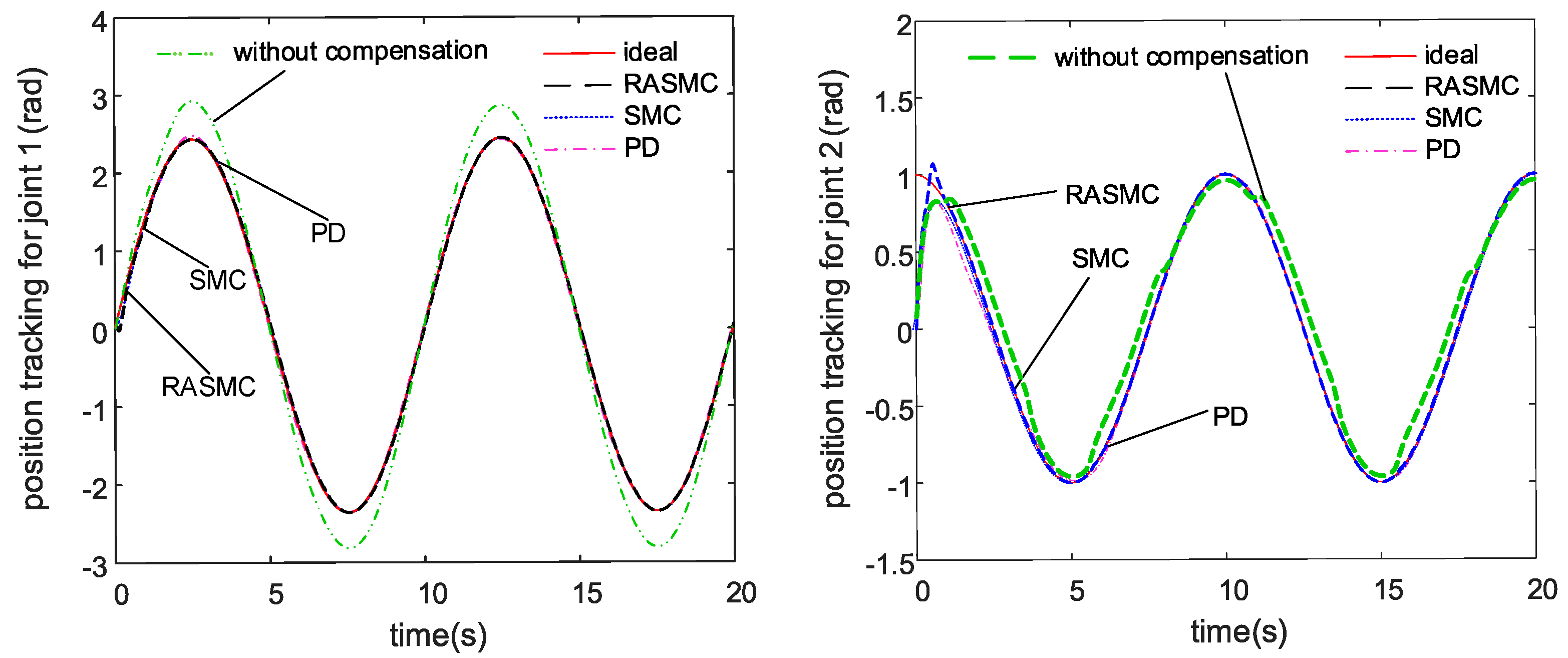
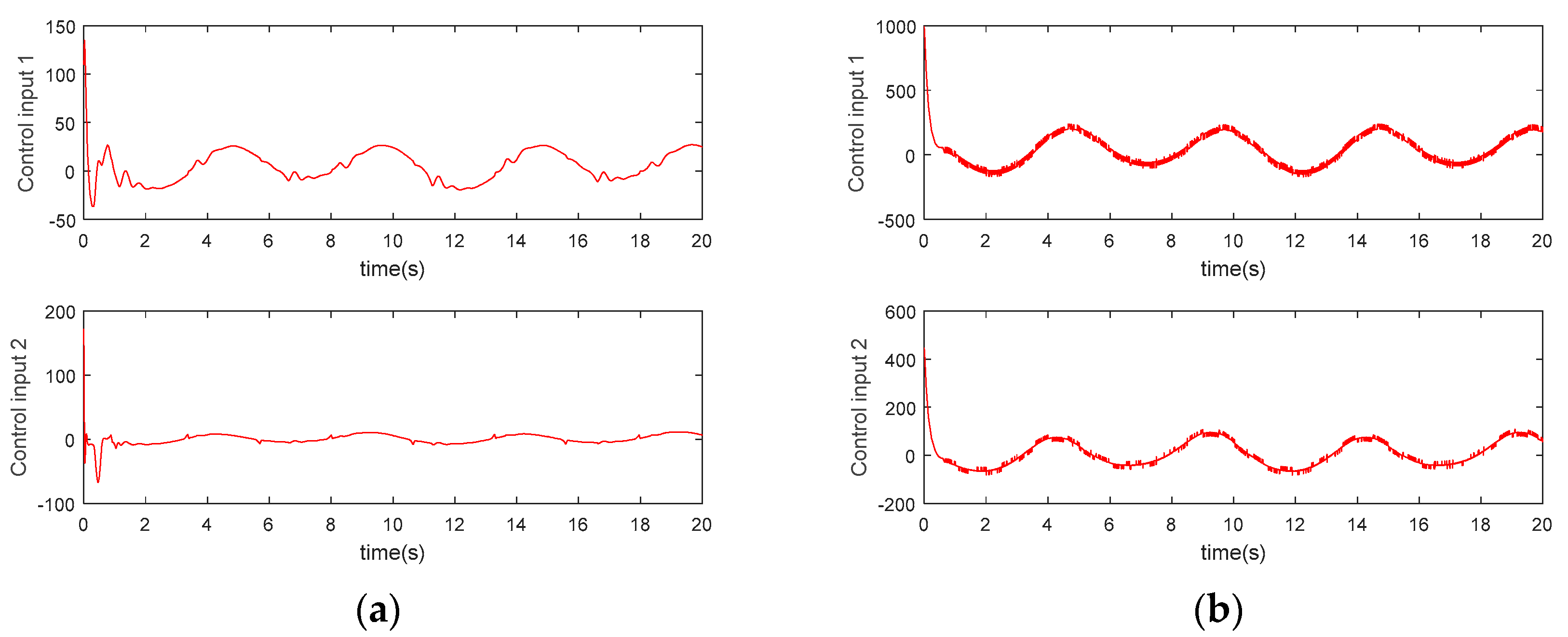
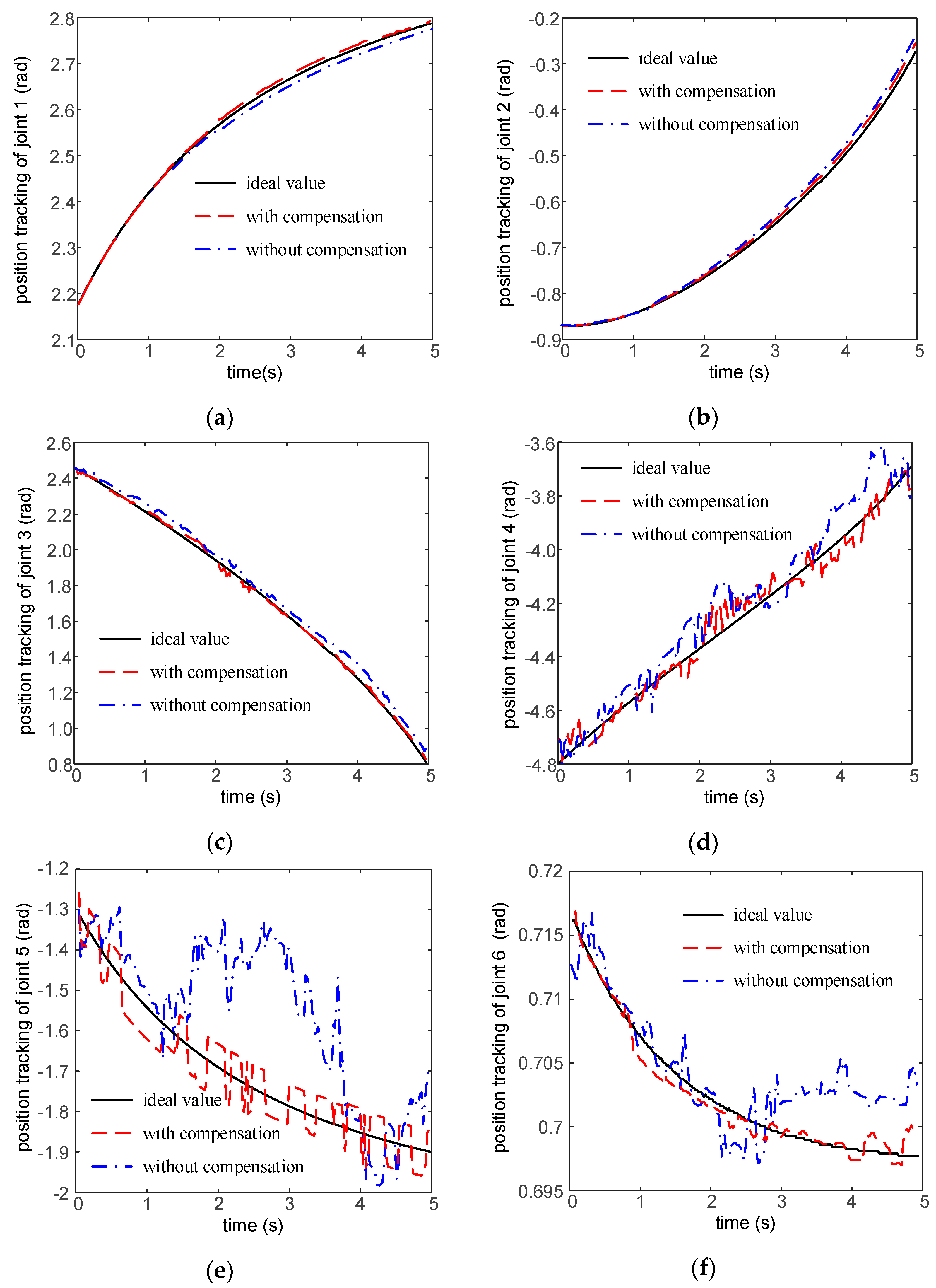
4.1. Simulation Analysis

To verify the effectiveness of the proposed intelligent control method using machine learning based on RBFNNs, the two-link robot manipulator model of FFSGR shown in Figure 6 was utilized. Based on Reference [10], the dynamic equation for the two-link robot manipulators with joint friction and external disturbance can be described as follows:

$$M\left(q\right)=\left[\begin{array}{cc}{M}_{11}& M_{12}\\ M_{21}& M_{22}\end{array}\right], C\left(q\right)=\left[\begin{array}{cc}{C}_{11}& C_{12}\\ C_{21}& C_{22}\end{array}\right], G\left(q\right)=\left[\begin{array}{c}{G}_1\\ G_2\end{array}\right], F\left(\dot{q}\right)=\left[\begin{array}{c}{F}_1\\ F_2\end{array}\right], {\tau }_d=\left[\begin{array}{c}{\tau }_1\\ {\tau }_2\end{array}\right]$$

(47)

and

$$\begin{array}{l}\{\begin{array}{c}{M}_{11}=\left(m_1+m_2\right)l_1^2+m_2{l}_2^2+2m_2{l}_1{l}_2\cos \left(q_2\right)\\ M_{22}=m_2{l}_2^2\\ M_{12}=M_{21}=m_2{l}_2^2+m_2{l}_1{l}_2\cos \left(q_2\right)\end{array},\{\begin{array}{c}{C}_{11}=-m_2{l}_1{l}_2\sin \left(q_2\right){\dot{q}}_2\\ C_{12}=-m_2{l}_1{l}_2\sin \left(q_2\right)\left({\dot{q}}_1+{\dot{q}}_2\right)\\ C_{21}=m_2{l}_1{l}_2\sin \left(q_2\right){\dot{q}}_1,C_{22}= 0\end{array}\\ \{\begin{array}{c}{G}_1=\left(m_1+m_2\right)l_{1}g\cos \left(q_2\right)+m_2{l}_{2}g\cos \left(q_1+q_2\right)\\ G_2=m_2{l}_{2}g\cos \left(q_1+q_2\right)\end{array},\{\begin{array}{c}{F}_1=0.2sign\left({\dot{q}}_1\right)\\ F_2=0.2sign\left({\dot{q}}_2\right)\end{array},\{\begin{array}{c}{\tau }_1=0.5\sin (t)\\ {\tau }_2=0.5cos\left(t\right)\end{array}\end{array}$$

(48)

here $m_1$ and $m_2$ are the masses of joint 1 and joint 2, respectively; $l_1$ and $l_2$ are the length of joint 1 and joint 2, respectively; and g is the acceleration of gravity.

The parameters of the considered two-link robot manipulators are given as:

$$m_1=3\mathrm{kg}, m_2=2\mathrm{kg}, l_1=0.8\mathrm{m}, l_2=1\mathrm{m}, g=10\mathrm{m}/{\mathrm{s}}^2$$

(49)

The chosen dead zone parameters are:

$$d^{+}=13, d^{-}=-15, m\left(u_C\right)=u_C-d^{+}, n\left(u_C\right)=u_C+d^{-}$$

(50)

The parameter values used in the adaptive control system are:

$$c=diag\left[\begin{array}{cc}6& 6\end{array}\right], K_g=diag\left[\begin{array}{cc}30& 30\end{array}\right], K_s=diag\left[\begin{array}{cc}1& 1\end{array}\right]$$

(51)

The parameter values used in the RBFNNs are:

$$S=diag\left[\begin{array}{cc}400& 400\end{array}\right], T=diag\left[\begin{array}{cc}500& 500\end{array}\right], b_i=100, c_i=\left[\begin{array}{ccccccc}-50& -20& -10& 0& 10& 20& 40\\ -50& -20& -10& 0& 10& 20& 40\end{array}\right]$$

(52)

where the initial values of the weights are all 20.

The control objective was to control the joint angles of the two-link robot manipulators to follow the desired trajectories. The initial positions of the joints and the initial velocities of the joints were 0, while the desired position trajectories of the two-link robot manipulators were chosen as $q={\left[\begin{array}{cc}2\sin \left(0.2\pi t\right)& \cos \left(0.2\pi t\right)\end{array}\right]}^T$ (in radians).

As illustrated in Figure 7, due to the existence of dead zone dynamics, there was a large error between the actual output of the joint driver and the ideal output of the controller. The existence of this error significantly affected the performance of the controller, so it was necessary to identify and compensate for the dead zone characteristics.

As shown in Figure 8, the designed identification method based on RBFNNs can converge in limited time, and the dead zone characteristics can be accurately identified. To eliminate the influence of a dead zone on system performance, the identification results should be added to the controller as a compensation term.

The position tracking results are shown in Figure 9. Due to the existence of a dead zone, the control method without compensation has an obvious steady-state error. All three methods can make the system stable, namely, PD (proportional differential), SMC (sliding mode control), and RASMC (robust adaptive sliding mode control). For joint 1, the convergence time of the three methods was 3 s, 1.1 s, and 0.8 s, respectively. For joint 2, the convergence time of the three methods is 0.9 s, 2.8 s, and 6.4 s, respectively. The maximum steady-state error was reduced from 0.06 rad to 0.015 rad. It was shown that the proposed RASMC method was superior to the other two methods in convergence speed, which is consistent with the theoretical analysis.

According to Figure 10, with the estimation and compensation of the dead zone, the gain of a robust term in RASMC was greatly reduced compared to that in SMC, and the chattering was significantly weakened. In this way, the control input was smoother, and the control performance was improved significantly. The necessity for dead zone identification and feedforward compensation was further highlighted in the experimental tests described in the following.

4.2. Experiment Validation

In order to further verify the effectiveness and practicability of the proposed control method, a robot grinding experiment was carried out in the lab. As shown in Figure 11, the experimental setup was based on an automatic production line for the intelligent manufacture of high-end equipment, which was independently developed by the National Engineering Laboratory for Robot Vision Perception and Control Technology. The robot model was the MH-24 of Yaskawa, as shown in Figure 11 (left panel). Six drivers were connected to the industrial computer through the Ethercat bus, and each joint motor was controlled by an industrial computer. The workpiece for grinding was a cylinder block from an automobile engine. The sampling frequency was 100 Hz, and the grinding task for the robot was to grind 300 mm along a straight line in 5 s.

In the experiment, a limiter was applied to the output of the first joint controller to simulate the dead zone. The upper limit was 0.8, and the lower limit was −2. As can be seen from Figure 12, due to the fact of a certain delay, there was a large identification error at the moment of the upper and lower limit switching. When the system was in a steady state, the method based on the RBFNNs designed in this paper could identify the dead zone accurately. The peak value of the absolute value of the steady state error was 0.08.

Figure 13 shows that all six joints were stable under the action of the controller. Taking the most fluctuating joint (4) as an example, the peak value of the steady-state error was 1.21 rad without compensation and 0.96 rad with compensation, which represents a decrease of 21%. The results clearly show that the system’s steady-state performance and grinding accuracy were improved with the introduction of dead zone compensation. The same conclusion can also be determined from the other five joints. The last three joints fluctuated sharply because they were close to the polished end. The sixth joint (that is, the last joint) was directly connected with the grinding head. During the polishing process, the position of this joint remained basically unchanged, so the range of the joint displacement’s change was very small.

5. Conclusions

In order to achieve high-precision grinding and polishing operations for robots and improve the processing accuracy of workpieces, accurate trajectory tracking performance is a key issue that must be considered. Focusing on non-linearity factors, such as dead zones, backlash, and saturation in robotic systems, this paper proposed a machine-learning-based non-linear identification method to identify all kinds of actuator non-linearities online. For accurate identification, an adaptive sliding mode trajectory tracking control system was designed. Meanwhile, the results of identification were fed to the controller to compensate the actuator’s non-linearity online, thereby reducing the gain of the sliding mode’s switching term. Thanks to the robustness of the sliding mode’s control, the chattering phenomenon and fluctuation of the control torque were effectively weakened. Thus, the performance of the control system was significantly improved. The simulation results show that the convergence time of the system was reduced from 1.1 to 0.8 s, and the maximum steady-state error was reduced from 0.06 to 0.015 rad, which sped up the stabilization rate of the system and reduced steady-state errors.

The results of engine cylinder grinding experiments show that dead zones can be accurately estimated. This control scheme, based on dead zone compensation, can reduce steady-state errors from 1.21 to 0.96 rad, which represents a decrease of 21%. Hence, this scheme can improve the grinding accuracy and ensure the smooth completion of grinding.

References

1. Li, W.L.; Xie, H.; Zhang, G.; Yan, S.J.; Yin, Z.P. 3-D Shape Matching of a Blade Surface in Robotic Grinding Applications. IEEE/ASME Trans. Mechatron. 2016, 21, 2294–2306. [Google Scholar] [CrossRef]
2. Ng, W.X.; Chan, H.K.; Teo, W.K. Programming a robot for conformance grinding of complex shapes by capturing the tacit knowledge of a skilled operator. IEEE Trans. Autom. Sci. Eng. 2017, 14, 1020–1030. [Google Scholar] [CrossRef]
3. Jia, L.; Wang, Y.N.; Zhang, H.; Liu, L. Machine Learning-based Robust Adaptive Control for FFSGR with Actuator Dead zone. In Proceedings of the 13th World Congress on Intelligent Control and Automation (WCICA), Changsha, China, 4–8 July 2018; IEEE: Washington, DC, USA, 2018; pp. 1349–1352. [Google Scholar]
4. Hamelin, P.; Bigras, P.; Beaudry, J. Multiobjective optimization of an observer-based controller: Theory and experiments on an underwater grinding robot. IEEE Trans. Control Syst. Technol. 2014, 22, 1875–1882. [Google Scholar] [CrossRef]
5. Li, W.L.; Xie, H.; Zhang, G. Hand–Eye Calibration in Visually-Guided Robot Grinding. IEEE Trans. Cybern. 2016, 46, 2634–2642. [Google Scholar] [CrossRef] [PubMed]
6. Yu, P. Research and application of piping inside grinding robots in nuclear power plant. Energy Procedia 2017, 127, 54–59. [Google Scholar] [CrossRef]
7. Friedl, B. Advanced Control System Design; Prentice-Hall: Englewood Cliffs, NJ, USA, 1996. [Google Scholar]
8. Zhonghua, W.; Bo, Y.; Lin, C.; Shusheng, Z. Robust adaptive dead zone compensation of DC servo system. IEE Proc. Control Theory Appl. 2006, 153, 709–713. [Google Scholar] [CrossRef]
9. Park, S.H.; Han, S.I. Robust-tracking control for robot manipulator with dead zone and friction using backstepping and RFNN controller. IET Control Theory Appl. 2011, 5, 1397–1417. [Google Scholar] [CrossRef]
10. Lewis, F.L. Dead zone compensation in motion control systems using neural networks. IEEE Trans. Autom. Control 2000, 45, 602–613. [Google Scholar]
11. Tao, G.; Kokotovic, P.V. Adaptive control of plants with unknown dead-zones. IEEE Trans. Autom. Control 1994, 39, 59–68. [Google Scholar]
12. Zhang, Z.; Xu, S.; Zhang, B. Exact tracking control of non-linear systems with time delays and dead-zone input. Automatica 2015, 52, 272–276. [Google Scholar] [CrossRef]
13. Saeki, M.; Wada, N.; Satoh, S. Stability analysis of feedback systems with dead-zone non-linearities by circle and Popov criteria. Automatica 2016, 66, 96–100. [Google Scholar] [CrossRef]
14. Cui, G.; Wang, Z.; Zhuang, G.; Li, Z.; Chu, Y. Adaptive decentralized NN control of large-scale stochastic non-linear time-delay systems with unknown dead-zone inputs. Neurocomputing 2015, 158, 194–203. [Google Scholar] [CrossRef]
15. Gao, Y.; Tong, S.; Li, Y. Fuzzy adaptive output feedback DSC design for SISO non-linear stochastic systems with unknown control directions and dead-zones. Neurocomputing 2015, 167, 187–194. [Google Scholar] [CrossRef]
16. Shi, W. Adaptive fuzzy control for multi-input multi-output non-linear systems with unknown dead-zone inputs. Appl. Soft Comput. 2015, 30, 36–47. [Google Scholar] [CrossRef]
17. Li, Z.; Su, C.Y. Neural-adaptive control of single-master–multiple-slaves teleoperation for coordinated multiple mobile manipulators with time-varying communication delays and input uncertainties. IEEE Trans. Neural Netw. Learn. Syst. 2013, 24, 1400–1413. [Google Scholar] [PubMed]
18. Li, Z.; Chen, Z.; Fu, J. Direct adaptive controller for uncertain MIMO dynamic systems with time-varying delay and dead-zone inputs. Automatica 2016, 63, 287–291. [Google Scholar] [CrossRef]
19. Zuo, Z.; Li, X.; Shi, Z. L1 adaptive control of uncertain gear transmission servo systems with dead zone non-linearity. ISA Trans. 2015, 58, 67–75. [Google Scholar] [CrossRef] [PubMed]
20. Wu, L.B.; Yang, G.H.; Wang, H. Adaptive fuzzy asymptotic tracking control of uncertain nonaffine non-linear systems with non-symmetric dead-zone non-linearities. Inf. Sci. 2016, 348, 1–14. [Google Scholar] [CrossRef]
21. Wu, B.; Cao, X.; Xing, L. Robust adaptive control for attitude tracking of spacecraft with unknown dead-zone. Aerosp. Sci. Technol. 2015, 45, 196–202. [Google Scholar] [CrossRef]
22. Wu, L.B.; Yang, G.H. Robust adaptive fault-tolerant tracking control of multiple time-delays systems with mismatched parameter uncertainties and actuator failures. Int. J. Robust Non-Linear Control 2015, 25, 2922–2938. [Google Scholar] [CrossRef]
23. Deng, W.; Yao, J.; Ma, D. Robust adaptive asymptotic tracking control of a class of non-linear systems with unknown input dead-zone. J. Frankl. Inst. 2015, 352, 5686–5707. [Google Scholar] [CrossRef]
24. Zhang, Z.; Xu, S.; Zhang, B. Asymptotic tracking control of uncertain non-linear systems with unknown actuator non-linearity. IEEE Trans. Autom. Control 2014, 59, 1336–1341. [Google Scholar] [CrossRef]
25. Wang, H.; Chen, B.; Liu, X. Robust adaptive fuzzy tracking control for pure-feedback stochastic non-linear systems with input constraints. IEEE Trans. Cybern. 2013, 43, 2093–2104. [Google Scholar] [CrossRef] [PubMed]
26. Li, Y.; Tong, S.; Li, T. Observer-based adaptive fuzzy tracking control of MIMO stochastic non-linear systems with unknown control directions and unknown dead zones. IEEE Trans. Fuzzy Syst. 2015, 23, 1228–1241. [Google Scholar] [CrossRef]
27. Wu, L.B.; Yang, G.H. Adaptive fuzzy tracking control for a class of uncertain nonaffine non-linear systems with dead-zone inputs. Fuzzy Sets Syst. 2016, 290, 1–21. [Google Scholar] [CrossRef]
28. Li, Y.; Tong, S. Hybrid adaptive fuzzy control for uncertain MIMO non-linear systems with unknown dead-zones. Inf. Sci. 2016, 328, 97–114. [Google Scholar] [CrossRef]
29. Wu, L.; Yang, X.; Lam, H.K. Dissipativity analysis and synthesis for discrete-time T–S fuzzy stochastic systemswith time-varying delay. IEEE Trans. Fuzzy Syst. 2014, 22, 380–394. [Google Scholar] [CrossRef]
30. Li, Y.; Tong, S. Adaptive fuzzy output-feedback control of pure-feedback uncertain non-linear systems with unknown dead zone. IEEE Trans. Fuzzy Syst. 2014, 22, 1341–1347. [Google Scholar] [CrossRef]
31. Tong, S.; Wang, T.; Li, Y. Adaptive neural network output feedback control for stochastic non-linear systems with unknown dead-zone and unmodeled dynamics. IEEE Trans. Cybern. 2014, 44, 910–921. [Google Scholar] [CrossRef]
32. Sui, S.; Tong, S.; Li, Y. Observer-based adaptive fuzzy decentralized control for stochastic large-scale non-linear systems with unknown dead-zones. Inf. Sci. 2014, 259, 71–86. [Google Scholar] [CrossRef]
33. Wu, J.; Chen, W.; Yang, F. Global adaptive neural control for strict-feedback time-delay systems with predefined output accuracy. Inf. Sci. 2015, 301, 27–43. [Google Scholar] [CrossRef]
34. Zhao, Z.; Wang, X.; Zhang, C. Neural network based boundary control of a vibrating string system with input deadzone. Neurocomputing 2018, 275, 1021–1027. [Google Scholar] [CrossRef]
35. Zhao, X.; Shi, P.; Zheng, X. Adaptive tracking control for switched stochastic non-linear systems with unknown actuator dead-zone. Automatica 2015, 60, 193–200. [Google Scholar] [CrossRef]
36. He, W.; Dong, Y.; Sun, C. Adaptive neural network control of unknown non-linear affine systems with input dead zone and output constraint. ISA Trans. 2015, 58, 96–104. [Google Scholar] [CrossRef] [PubMed]
37. Li, S.; Gong, M.Z.; Liu, Y.J. Neural network-based adaptive control for a class of chemical reactor systems with non-symmetric dead-zone. Neurocomputing 2016, 174, 597–604. [Google Scholar] [CrossRef]
38. Wang, H.Q.; Chen, B.; Lin, C. Adaptive neural tracking control for a class of stochastic non-linear systems with unknown dead-zone. Int. J. Innov. Comput. Inf. Control 2013, 9, 3257–3269. [Google Scholar]
39. Hsu, C.F.; Lin, C.M.; Yeh, R.G. Supervisory adaptive dynamic RBF-based neural-fuzzy control system design for unknown non-linear systems. Appl. Soft Comput. 2013, 13, 1620–1626. [Google Scholar] [CrossRef]
40. Han, S.I.; Lee, J.M. Backstepping sliding mode control with FWNN for strict output feedback non-smooth non-linear dynamic system. Int. J. Control. Syst. 2013, 11, 398–409. [Google Scholar] [CrossRef]
41. Van, P.C.; Wang, Y.N. Robust Adaptive Trajectory Tracking Sliding mode control based on Neural networks for Cleaning and Detecting Robot Manipulators. J. Intell. Robot. Syst. 2015, 79, 101–114. [Google Scholar]
42. Lu, Y.; Liu, J.K.; Sun, F.C. Actuator non-linearities compensation using RBF neural networks in robot control system. In Proceedings of the Multiconference on Computational Engineering in Systems Applications (IMACS), Beijing, China, 4–6 October 2006; Volume 1, pp. 231–238. [Google Scholar]
Figure 1. A free-form surface grinding robot system.
Applsci 09 03837 g001
Figure 2. Non-symmetric dead zone non-linearity.
Applsci 09 03837 g002
Figure 3. Dead zone inverse.
Applsci 09 03837 g003
Figure 4. Dead zone compensation scheme.
Applsci 09 03837 g004
Figure 5. Structure block diagram of the control system.
Applsci 09 03837 g005
Figure 6. Two-link robotic manipulator model of free form surface grinding robots(FFSGRs).
Applsci 09 03837 g006
Figure 7. Input signal tracking performance of joint 1 (left) and joint 2 (right) without dead zone compensation.
Applsci 09 03837 g007
Figure 8. The estimated performance of the dead zone characteristics of joint 1 (left) and joint 2 (right).
Applsci 09 03837 g008
Figure 9. Position tracking performance of joint 1 (left) and joint 2 (right).
Applsci 09 03837 g009
Figure 10. (a) Control inputs of robust adaptive sliding mode control (RASMC); (b) Control inputs of sliding mode control (SMC).
Applsci 09 03837 g010
Figure 11. Experimental device diagram of the free form surface grinding robots(FFSGRs) (a) and engine cylinder block grinded in experiments (b).
Applsci 09 03837 g011
Figure 12. Dead zone non-linearity estimation performance of joint 1 (a) and estimation error (b).
Applsci 09 03837 g012
Figure 13. Position tracking performance of joint 1 (a), joint 2 (b), joint 3 (c), joint 4 (d), joint 5 (e), joint 6 (f).
Applsci 09 03837 g013