Target Points Tracking Control for Autonomous Cleaning Vehicle Based on the LSTM Network

Abstract

In order to efficiently and exactly in tracking the desired path points, autonomous cleaning vehicles have to adapt their own behavior according to the perceived environmental information. This paper proposes a target points tracking control algorithm based on the Long Short-Term Memory network, which can generate the speed and yaw rate to arrive at the target point in real time. The target point is obtained by a parameter named foresight distance that is deduced based on the fuzzy control, whose inputs are the speed and yaw rate of the vehicle at the current point. The effectiveness of the proposed algorithm is illustrated by the simulation and field experiments. Compared with other classical algorithms, this algorithm can track the point sequence on straight path and multiple curvature path more accurately. The field experiment indicates the proposed controller is efficient in following the pre-defined path points, furthermore, it can make the autonomous cleaning vehicle run smoothly in the path which is disturbed by bounded disturbances. The distance errors can meet the actual requirement of the cleaning vehicle during the tracking process.

1. Introduction

With the continuous development of advanced technologies such as Information Technology (IT), sensor technology, system engineering, and artificial intelligence, Intelligent Transportation System (ITS) has attracted more and more researchers’ attention, especially the design of automatic mobile robots and mobile systems [1]. One of the main hotspots in the field of autonomous mobile robots research is to design a target point tracking controller [2,3,4,5], which focuses on reaching the pre-defined point through longitudinal and lateral control of the vehicle [6], thus achieving a whole path points tracking in the given time. To be specific, the longitudinal controller is responsible for adjusting the vehicle’s cruise velocity while the lateral controller steers the vehicle’s wheels for trajectory tracking [7,8]. Therefore, the resulting control output should minimize the difference between the actual and expected points with respect to the lateral distance and the vehicle heading, and should ensure that the actual paths are smooth. However, for automatic cleaning robot, there is a strong coupling relationship between the longitudinal and lateral dynamics of the vehicle whose dynamic response is very complicated during the cleaning process, because its running involves sprinkling, vacuuming and scrubbing [9]. So the kinematic or dynamic model of the cleaning vehicle is complex [10], and to determine an appropriate target points tracking control algorithm is difficult.

At present, many scholars have studied target points tracking methods based on varied types of models such as geometric, kinematic and dynamic model or combination of them. Compared with the controller based on complex dynamic model, the controllers based on geometry and motion models are easier to implement and more robust to path curvature. In addition, the latter are more suitable for lower velocity driving because they do not consider the internal force of the whole vehicle system. However, the tracking accuracy of the controller based on dynamic model is usually better at higher speed, because the controller gives priority to the non-linear vehicle dynamic.

Existing tracking methods concretely include PID control [11], fuzzy control [12,13], optimal control [14], pure pursuit control [15], neural network control [16,17], and so on. They improve the goal points tracking performance for automatic vehicles in different aspects. In [11], a classical PID approach is proposed for the path tracking controller, which utilizes a simple linearized model consisting of an integrator and a delay to simulate a mobile robot. This experimental results demonstrate the good tracking performance and robustness of the proposed controller. The advantage of fuzzy control is that it does not require precise kinematics model or dynamic model for robots, reference [12] combines the linear regulator theory with Takagi-Sugeno fuzzy methodology and proposes a method to fulfil path tracking of nonlinear systems. It is worth mentioning that this method is easy to implement due to the use of linear control techniques. Reference [14] requires the vehicle to run at low speed, so the dynamic properties have little influence on the path tracking behavior. In [14], an optimal controller is designed to minimize the orientation error and the offset from a path. The controller structure is defined in terms of the running speed of the vehicle. Thus, it has the superiority of being flexible for speed changes, but the simulation or experiment performances of the controller are not specifically described in the text. Pure pursuit control [15] presents a steering control law for automatic vehicles according to the geometric relation between the ego-vehicle and the desire tracking path points. A parameter named preview distance is usually used to obtain the control variables and it has certain potentially abilities to extend from simple circular arc calculations to much more complex geometric theorems. Although the above methods can achieve good tracking results under specific conditions, some pre-defined path points used are too idealized. Since most of the path points currently used for tracking are obtained by smoothing and filtering from the original path points, which are collected by the map building. The original path usually has some noise points. It is still unknown whether the above methods can maintain a good tracking effect on the path with bounded disturbance, so the robustness of the target point tracking control algorithm remains to be proven. In addition, each algorithm has its own advantages and application occasions. If we can directly extract their good effect data without the tedious analysis process and construct a new control algorithm based on these existing data, it would be a new breakthrough in the field of the automatic control.

According to the universal approximation theorem [18], artificial neural network (ANN) has the potent ability to approximate the nonlinear system and it is considered as an effective approach to deal with complex problems. Related research in neural networks has shown exemplary results in the field of tracking control of wheeled mobile robot [19] and quadrotors [20], which illustrate the power of learning features directly from the data in the area of deep-learning. A unified robust neural network based control scheme is presented for trajectory tracking of a wheeled mobile robot with unknown parameters in reference [19], the proposed controller has a good performance on the steady-state errors and control inputs in both tracking and stabilization problems. Reference [20] proposes a DNN-based reference learning method that can learn the flight data and improve tracking performance in the quadrotor system, because of its superior capability of approximating abstract. Reference [16] proposes a novel path points tracking method based on learning, which combines the Stanley method with a Neural Dynamic Programming (NDP) algorithm perfectly. Although this method demonstrates state-of-the-art performance, the slight vibration is existed during the path tracking process according to the comprehensive simulation experiment. Due to their success in many applications, this paper chooses artificial neural network in the form of a Long Short-Term Memory (LSTM) network as the basis to study the target points tracking control algorithm, for the reason that path points can be treated as time sequence data in tracking. And to the best of our knowledge, the LSTM framework has not been designed for target points tracking control algorithm to predict the vehicles’ speed and yaw rate.

In this paper, we consider the problem of autonomous mobile cleaning robot in target points tracking, where the running speed is relatively lower than other scenarios, but the accuracy of the tracking process is higher because it involves cleaning efficiency. Inspired by the pure pursuit algorithm, we use a key parameter of this algorithm, foresight distance, which simulates the vision of the driver in driving and has the bionic characteristics. The foresight distance can be obtained by the fuzzy control, its inputs are the current velocity and yaw rate of the vehicle, and its output is an appropriate target foresight distance. After setting a suitable foresight distance, a simple geometric method is intended for obtaining the target point which is relative to the current vehicle position. In order to arrive at this target point, two-layer LSTM network controller is proposed to adjust the autonomous vehicle’s speed and yaw rate simultaneously and intelligently to reduce the lateral error of the path points tracking. The LSTM model has been trained in proper times based on abundant and good sample data, then the kinematic model of automatic vehicle are established and simulation experiments are carried on two typical paths. The simulation results are compared with the results of three effective control algorithms, and the advantages of the proposed algorithm are analyzed. Beyond that, this paper examines the effectiveness of the algorithm on a cleaning vehicle, studies the variation of velocity and foresight distance in the tracking, and evaluates its performance by the distance deviation of the straight line and the turning section in the field experiment. The real vehicle experiment result shows that the proposed controller is efficient not only in tracking the pre-defined path points smoothly but also in not affecting by the path noise points.

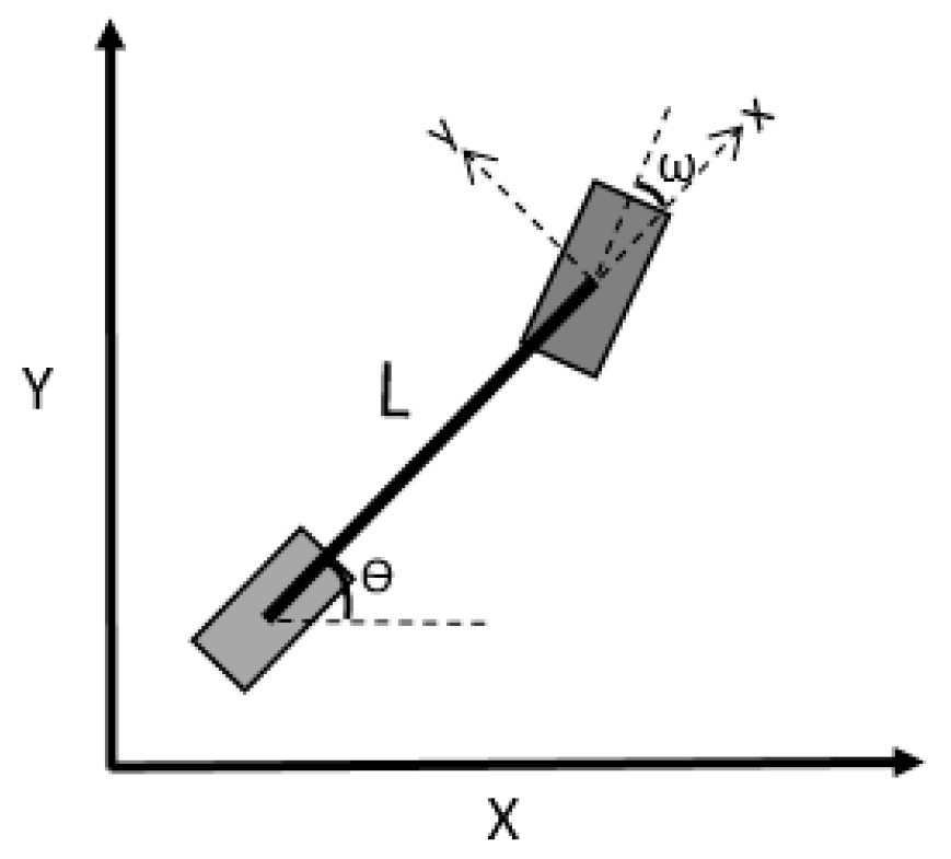
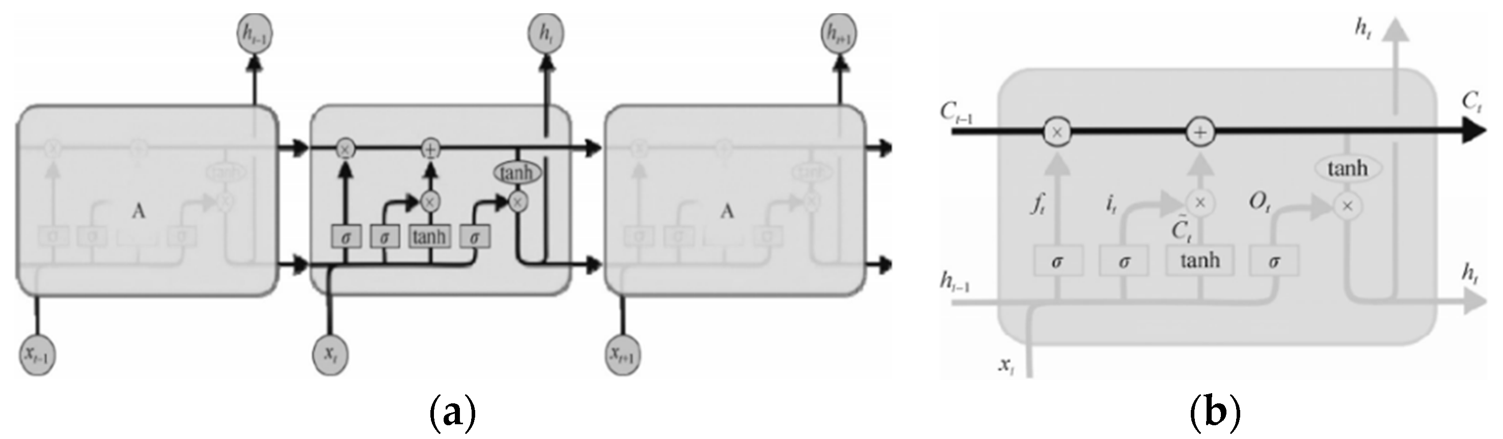
The rest of this article is structured as follows. In Section 2, we briefly review the technical background of the vehicle model, stability condition and the chain structure of LSTM. Section 3 describes the proposed tracking algorithm, which includes the discrimination of the foresight distance, the system description and the detailed network structure. In Section 4, the simulation and field experiments results are presented and Section 5 concludes this paper.

2. Technical Background

In this section, a brief review of the vehicle model and stability condition used in this paper will be analyzed firstly. Then the brief chain structure of LSTM and detail of the process in the information transmission are presented.

2.1. Vehicle Model and Stability Condition Analysis

When deriving the target points tracking control algorithm, the kinematic vehicle model [21] is used. The kinematic vehicle model is based on the Ackermann steering geometry that assumes the line perpendicular to each wheel should intersect at the center of the turning arc of the vehicle with a turning radius of R. Vehicle tires are regarded as rigid wheels and the lateral sliding between the tires and the ground is not considered. This model is usually used to obtain the steering control law as it can approximate the motion of the vehicle reasonably well at moderate steering angles and low velocities. The kinematics model of the two-wheel vehicle is simplified as shown in Figure 1.

The vehicle is described with two sets of Cartesian coordinates, local (x-y) and global (X-Y). Local coordinate is regarded as a moving coordinate with respect to the global coordinate because the vehicle is moving constantly. Supposing the speed of the vehicle (v) in the body frame is purely in x-direction. The relationship between the front wheel steering angle $\omega$ and the vehicle’s yaw $\theta$ is established as below. The L is the wheelbase, the ${\theta }^{\prime }(t)$ is the yaw rate, $x^{\prime }(t)$ is the X-direction speed and $y^{\prime }(t)$ is the Y-direction speed. The following relations can be obtained by the kinematic analysis.

$$x^{\prime }(t)=v\sin \theta$$

(1)

$$y^{\prime }(t)=v\cos \theta$$

(2)

$${\theta }^{\prime }(t)=\frac{v\tan \omega }{L}$$

(3)

The steering wheels of the cleaning vehicle is driven by stepping motors, whose speeds are proportional to the output of the controllers, so the whole steering system of the cleaning vehicle can be regarded as the first order inertia link, its formula is

$$\dot{\omega }=-\frac{1}{T}(\omega -{\omega }_U).$$

(4)

The ${\omega }_U$ is the target angle of front wheel, T is the time constant in the first order inertia link. The relationship between the curvature of turning and front wheel angle ω is as follows

$$\gamma =\frac{\tan \omega }{l}.$$

(5)

The γ is the actual turning curvature. When the front wheel angle is small, the above formula can be linearized as $\gamma =\frac{\omega }{l}$, so the changes of the turning curvature for the cleaning vehicle also be regarded as the first order inertia link.

$$\dot{\gamma }=-\frac{1}{T}(\gamma -{\gamma }_U)$$

(6)

The ${\gamma }_U$ is the target turning curvature, the ${\theta }^{\prime }(t)$ in the kinematics formula can be regard as ${\theta }^{\prime }(t)=v\gamma$. According to the method adopted in reference [22], when the model is in equilibrium $y^{\prime }(t)=0$ and $\omega =2/\pi$, the system characteristic polynomial is

$$f(\lambda )={\lambda }^3-\frac{1}{T}({\phi }_{\gamma }-1){\lambda }^2-\frac{v}{T}{\phi }_{\theta }\lambda +\frac{v^2}{T}{\phi }_y.$$

(7)

According to Routh Criterion and the parameter $L_d$ in pure pursuit algorithm [23], we can get the condition of the system is in a stable state.

$$L_d\ge Tv$$

(8)

2.2. LSTM Network

LSTM (Long Short-Term Memory) neural network was proposed by Sepp Hochreiter and Jurgen Schmidhuber in 1997 [24]. It is an optimized RNN (Recurrent Neural Network) that is designed to treat for the time sequence data based on the recurrent framework. With the increase number of times of information transmission, RNN will have problems in learning to convey the information due to the gradient vanishing or exploding issue, but the LSTM network can avoid these difficulties perfectly. The most remarkable point of LSTM is its repeated neural network memory module, also known as the hidden layer which is no longer a simple neuron node; it’s a computing node with rich internal structure, which contains a self-connected memory cell and three “gates” that control the flow of information. The gates include input gate, output gate and forget gate. Due to their recurrent structure, even a single layer of LSTM nodes can be considered as a “deep” neural network. The structure of LSTM is shown in Figure 2.

At time step $t$, the calculation formulas of the $l$-th layer units can be expressed as:

$$f_t=\sigma (W_{xf}{x}_t+W_{hf}{h}_{t-1}+b_f)\hspace{1em}{i}_t=\sigma (W_{xi}{x}_t+W_{hi}{h}_{t-1}+b_i)$$

(9)

$${\tilde{C}}_t=\tanh (W_{xc}{x}_t+W_{hc}{h}_{t-1}+b_c)\hspace{1em}{C}_t=f_t\otimes C_{t-1}+i_t\otimes \widetilde{C_t}$$

(10)

$$o_t=\sigma (W_{xo}{x}_t+W_{ho}{h}_{t-1}+W_{co}{C}_t+b_o)\hspace{1em}{h}_t=o_t\otimes \tanh h(C_t)$$

(11)

where the vectors $f_t$, $i_t$, $o_t$, $C_t$ represent the activation of the forget, input, output gates, and memory cells, respectively. $W_{ab}$ terms denote the weight matrix between $a$ and $b$ (e.g., $W_{xi}$ is the weight matrix from the inputs $x_t$ to the input gate $i_t$), and these four weight matrixes are associated with the inputs $x_t$. The $b_{\alpha }$ describes the bias term of $\alpha$ with $\alpha \in \{i,f,C,O\}$, $\sigma$ is the logistic sigmoid function as $\sigma (x)=1/(1+e^{-x})$, and ‘$\otimes$’ denotes the Hadamard product. The multiplicate LSTMs model can be applied to solve many real-life time sequence modeling problems, and multiple LSTMs can be stacked or concatenated flexibly to form more complex structures.

3. Proposed Trajectory Tracking Control Algorithm

In this section, the method to determine the foresight distance is described, the preview point is selected, the target points tracking system is designed, the network structure, and training method of the LSTM algorithm are proposed.

3.1. Determination of the Foresight Distance

In practical application, an autonomous vehicle have to work on different curvature paths, so it needs a very robust tracking controller. Motivated by the pure pursuit algorithm [25,26,27], a key parameter of this algorithm, foresight distance, are used, which has been widely applied in the field of target points tracking. It simulates the vision of the driver during the driving and has the bionic characteristics.

The preview ability is very significant for target points tracking, but to select the foresight distance as a linear function of vehicle velocity is evidently not a good choice [28]. On the one hand, a shorter foresight distance provides a smaller tracking error for a vehicle, but its stability is affected. On the other hand, a longer foresight distance provides a smoother tracking performance, but it may cause cut corners disaster while executing turns. Therefore, the trade-off between stability and tracking performance is a thorny matter. As a result, a method to improve the tracking performance by preview distance based controller is proposed in this paper.

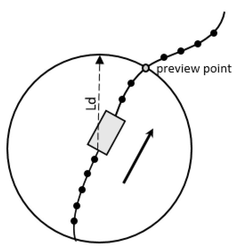
In order to closely approximate the continuous path, we divide the reference path into uniform points with index numbers, so the denser discretization of the path is realized. In this paper, the method of selecting the preview point is to draw a circle with radius $L_d$ centered on rear axle of the vehicle, as indicated in Figure 3. $L_d$ is the foresight distance obtained by the fuzzy control according to the real-time situation of the vehicle. A double-input and single-output structure is adopted, in which the inputs of the fuzzy controller are the current velocity $v$ and the yaw rate $\omega$ of the vehicle, and the output is an appropriate target foresight distance $L_d$.

To take the fuzzy set of speed grades as {Z, PS, PM, PB, PL}, its domain are [0, 1.0]. The fuzzy set of yaw rate grades is {NB, NM, NS, Z, PS, PM, PB}, its domain are [−90, 90], where B is Big; N is Negative; M is Middle; S is Small; Z is Zero; P is Positive; L is Large. To take the typical triangle function as the membership functions, and the fuzzy control rules will affect the outputs.

When designing the fuzzy control rules, the following principles are considered: (1) If the absolute value of $\omega$ is smaller, the $L_d$ is larger; If the absolute value of $\omega$ is larger, the $L_d$ is smaller. (2) Under the condition of satisfying the system stability, if the v of the vehicle is slower, the $L_d$ is smaller. If the v is faster, the $L_d$ is larger. The basic field of foresight distance $L_d$ is [0.1, 1.3] (/m) and the quantization level is {0.1, 0.4, 0.7, 1.0, 1.3} = {S, SM, M, ML, L} of fuzzy control, as shown in

Table 1. Foresight distance fuzzy control lookup table.

	$\mathit{\omega }$/(°)	NB	NM	NS	Z	PS	PM	PB
v/(m/s)
Z		S	S	SM	SM	SM	S	S
PS		S	SM	M	M	M	SM	S
PM		S	SM	M	ML	M	SM	S
PB		S	M	ML	L	ML	M	S
PL		SM	ML	L	L	L	ML	SM

. After that, the output from any input or combination of input fuzzy sets can be determined. Here, the “and” rule is used between two inputs. It is obvious that foresight distance, driving velocity, and the yaw rate are coordinated.

Based on the above method, the appropriate foresight distance can be determined according to different conditions in the process of goal points tracking.

3.2. Trajectory Tracking Control System Description

The main objective of this study is to design an adaptive controller that can determine the control variables ω and v for the autonomous cleaning vehicle to reach the goal points. LSTM network is robust and efficient for non-linear system control, which can make a series of non-linear transformations on the input data, and solve the problems of bad training approximation and generalization as much as possible. 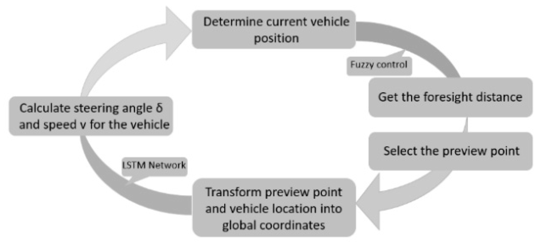The use of deep learning neural network provides possibilities for multiple types of complex function calculations [29,30]. Since the path points and some process variables during the tracking can be considered as the time sequence data intuitively, the LSTM network can be used for predicting the control variables of the cleaning vehicle. The overall structure of the target points tracking algorithm is shown in Figure 4.

Deep learning requires a large set of samples in order to converge to a solution without overfitting and to be well extended to the previously unseen samples. The training samples are collected from our own field and simulation experiments. In the field experiment, the cleaning vehicle should be pushed to create a pre-defined path firstly. Besides, the laser visual sensor and ultrasonic sensors can perceive and record the characteristics of the pre-defined path such as the passing path points (Containing noise points, which are the induction error of sensors), and the surrounding environment such as the location of walls. Then the traditional and improved pure pursuit [28] algorithms are separately used to obtain the sample velocity and sample yaw rate at each actual position of vehicle passed. The real difference between two methods lies in their foresight distance. Traditional pure pursuit algorithm with constant foresight distance performs well in the straight line path points, while the improved algorithm with dynamic foresight distance has good performance at the turning due to its linear function of vehicle velocity. Finally, when the detected wall is within 0.5 m around the vehicle, the vehicle velocity needs to be readjusted based on the aforementioned velocity by the following formula.

$$v_{final}=v_t\ast \left(\frac{d}{0.5}\right)$$

(12)

The $v_t$ is the speed obtained by the experimental tracking controller. The d is the minimum distance from the vehicle nose to the wall, and $\frac{d}{0.5}$ is equivalent to a decay factor that can reduce the speed of the vehicle at the appropriate times to ensure safety. The resulting velocity $v_{final}$ and yaw rate values will be fed into the neural network as the sample data (label). The simulation platform can extract more representative data through simulating cleaning routes in different environments by human intervention. Ultimately, 100 maps are analyzed, each with 500 different pre-defined path, for a total of 50,000 paths and about 100,000,000 path points, including diverse turning and straight path segments. About 20,000,000 groups of velocity and yaw rate sample data are obtained under two tracking algorithm.

At time t, the system supposes that the cleaning vehicle can determine the global coordinates of the target point $(x_{t\arg et},y_{t\arg et})$ in the pre-defined path detected by the sensors (e.g., laser sensor and ultrasonic sensors). Besides, it can get its owner accurate position $(x_c,y_c)$ based on the merge of gyroscopes, odometers, and amcl algorithm. According to the coordinate transformation relation, the angle ${\alpha }_t$ and distance $d_t$ between the current position and the target point can be acquired as Equations (13) and (14). It is stipulated that the positive value $\alpha$ representing the target point is on the left side of the vehicle, while the negative value $\alpha$ representing the target point is on the right side of the vehicle.

$${\alpha }_t={\tan }^{-1}\left(\frac{y_{t\arg et}-y_c}{y_{t\arg et}-x_c}\right)$$

(13)

$$d_t=\sqrt{{(x_{t\arg et}-x_c)}^2+{(y_{t\arg et}-y_c)}^2}$$

(14)

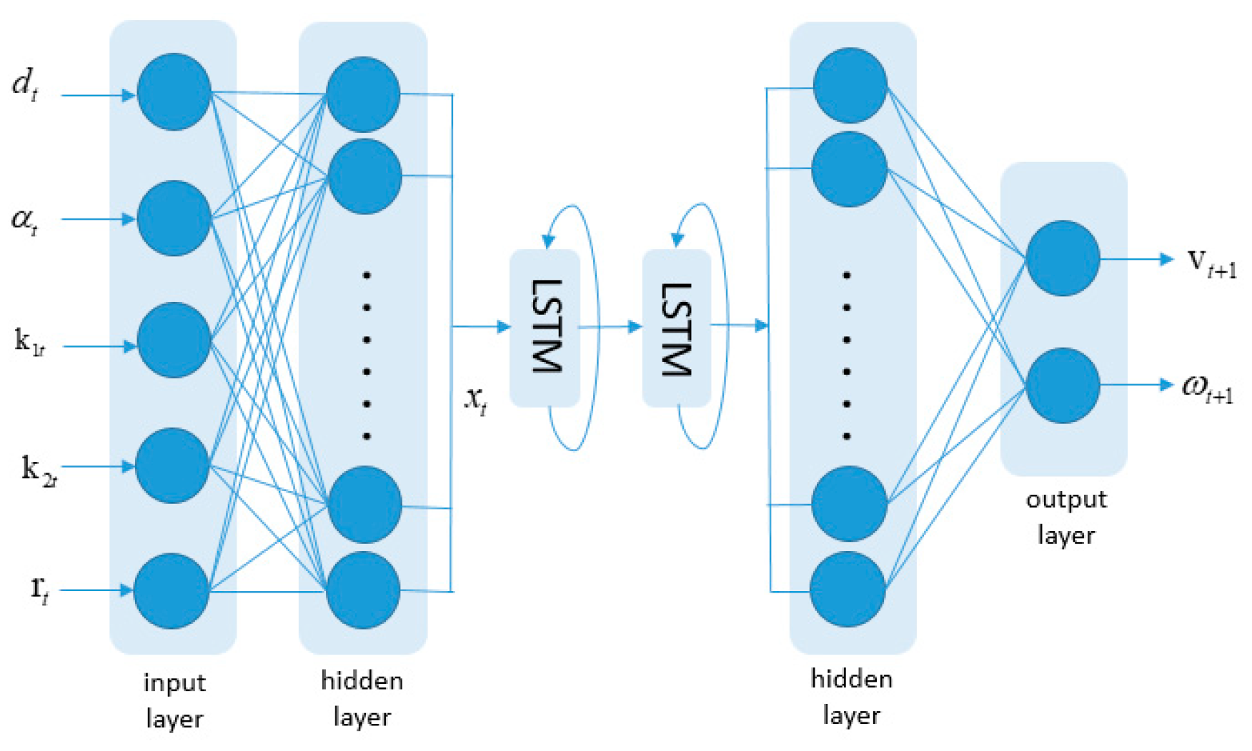
The set of the observations used for reaching the target point on the reference path at the time step t is given by: $O_t=\{{\alpha }_t,d_t,k_{1t},k_{2t},r_t\}$, The features of ${\alpha }_t$ as well as $d_t$ are chosen to replicate the driving habits of the human driver, because drivers tend to visually measure the distance and the angle to the target point. Then the speed and yaw rate are determined according to above three variables. $k_{1t}$, $k_{2t}$ represent the minimum distances from the obstructions to the two edges in front of the rectangular-shaped cleaning vehicle equipped with ultrasonic sensors. $r_t$ is a value detected by the laser, which stands for the distance from the obstructions to the vehicle nose. Considering the length and width of the vehicle and above five values comprehensively, the vehicle can control the speed and yaw rate more intelligently when turning or approaching obstacles. For example, if the vehicle’s length is too long to turn around a curve or the obstacle is too close to the vehicle’s body, the control variables need to be fine-tuned the control parameters. So the input of the LSTM network is the observations data $O_t$, whose features are scaled to remain in an acceptable range with respect to the activation function, and the output is the predicted data $M_{}$: $M=\{v_{final},\omega \}$, where, $v_{final}$ is the speed and $\omega$ is the yaw rate to reach the target point.

Figure 5 depicts the detail architecture of the proposed LSTM model, a two-layer deep LSTM network is used to build a structure for the input sequences in our network.

Appling the proposed LSTM network to the target points tracking algorithm can provide the cleaning vehicle with a robust controller, and at the same time promote the progress of tracking control algorithm greatly.

3.3. Network Structure

In this paper, deep-learning neural network can learn autonomously on the premise that the model knows the inputs and outputs, and it transforms the samples into some rules. After many iterations, the ability of neural network to recognize features increases gradually. The focus of the entire network learning process is to continuously optimize the learned laws based on the minimum condition of the loss function. Based on those rules, the model can not only predict what has been learned ahead, but also makes more reasonable predictions for the content that is not learned before.

After several tests, 256 features are extracted from the input layer, so the length of $x_t$ vector is 256. Then a two-layer LSTM architecture is used, since the large and complex trajectory training data need to be modeled to find more potential relationships of the temporal events in sequences. The two-layer is best for our task, which increasing the generalization capability of our model and expanding the network capacity as much as possible to capture the trajectory data. Finally, the hidden layer is used to transfer the 256-dimension of data into 2-dimension being consistent with the output layer.

The proposed network model is built using Python on Keras with a Tensorflow backend. Because there is still no known appropriate method for selecting correct hyper parameters for LSTM, so a variety of experiments are carried out and finally some parameters are selected with better performances. The training dataset is divided into batches of sequences of size n = 256. We use the popular zero-mean and unit variance to normalize the input data. During the training, the loss function is optimized as follows:

$$loss={\lambda }_1\frac{{\displaystyle {\sum }_{i=1}^n{(v_{final\_i}-v_i{}^{\prime })}^2}}{n}+{\lambda }_2{\displaystyle {\sum }_{i=1}^n\frac{{({\omega }_i-{\omega }_i{}^{\prime })}^2}{n}}.$$

(15)

where, $v_i$ and ${\omega }_i$ are the labels of the speed and yaw rate data in a batch, $v_i{}^{\prime }$ and ${\omega }_i{}^{\prime }$ are the predictive value obtained by the neural network. We set the weights ${\lambda }_1=0.4$ and ${\lambda }_2=0.6$ to reflect the importance of the yaw rate, which can influence the accuracy of path tracking, while the speed affects the efficiency of cleaning. For the minimization of the loss function, the Adam optimization is applied in the training process, with the dynamic learning rate start with 0.004 and decay with a rate of 0.0005, which can reduce the neural network training time without losing the prediction accuracy. The dropout rate is 0.8. In order to regularize the network, the L2 regularization is used. Combining all parameters and methods, the whole system model is optimized to improve the network performance.

4. Experiment and Analysis

In order to verify the performance of the proposed algorithm, the simulation platform and field experiment are used to test the target points tracking control capability of the cleaning vehicle in this section.

4.1. The Analysis of Simulation Performance

The kinematics model of a two-wheel vehicle is taken as the control object to validate the control performance of this algorithm in the simulation platform. The wheelbase of the vehicle is 1 m, the initial velocity is 0 m/s, the vehicle’s nose direction is X-axis positive direction and the initial position is (0,−1), so the initial position deviation is 1 m. The simulation experiments are carried out under the conditions of the straight path and the multiple curvature path.

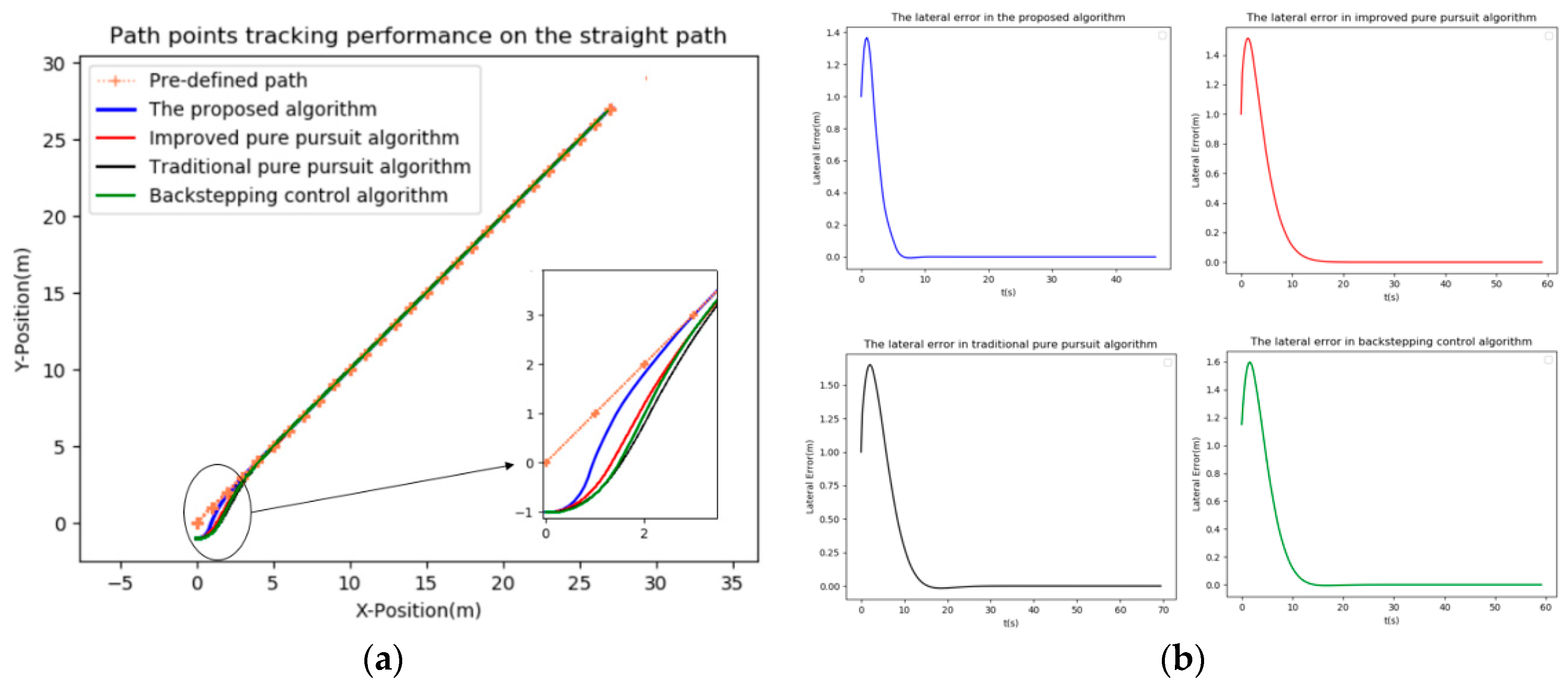
When tracking the straight path, the simulation performance is shown in Figure 6a. Four methods, namely the proposed method, the traditional pure pursuit method, the improved pure pursuit method and backstepping control method [31], are adopted to evaluate the tracking performances and are compared as well. The foresight distance and speed are set as constant values 0.7 m and 0.5 m/s in the traditional pure pursuit method. In the improved pure pursuit [25] method, the foresight distance is changed from constant to dynamic adjustment, which is a linear function of the vehicle velocity. In the backstepping control method, the desired configuration is the origin of the state space, while the initial configuration at t = 0 is x(0) = 0, y(0) = −1, θ(0) = 0, φ(0) = 0. We can intuitively see the difference among the above four controllers in Figure 6a, the proposed algorithm takes precedence over the other algorithms in tracking the pre-defined path points as it possesses the rapidity in the initial phase. The lateral error on the straight path in Figure 6b also shows that the proposed intelligent controller has lower lateral error when tracking some straight path points, followed by the improved pure pursuit method, while the traditional pure pursuit method and backstepping control method have the biggest lateral error. However, all four methods can perform well tracking abilities after reaching steady state.

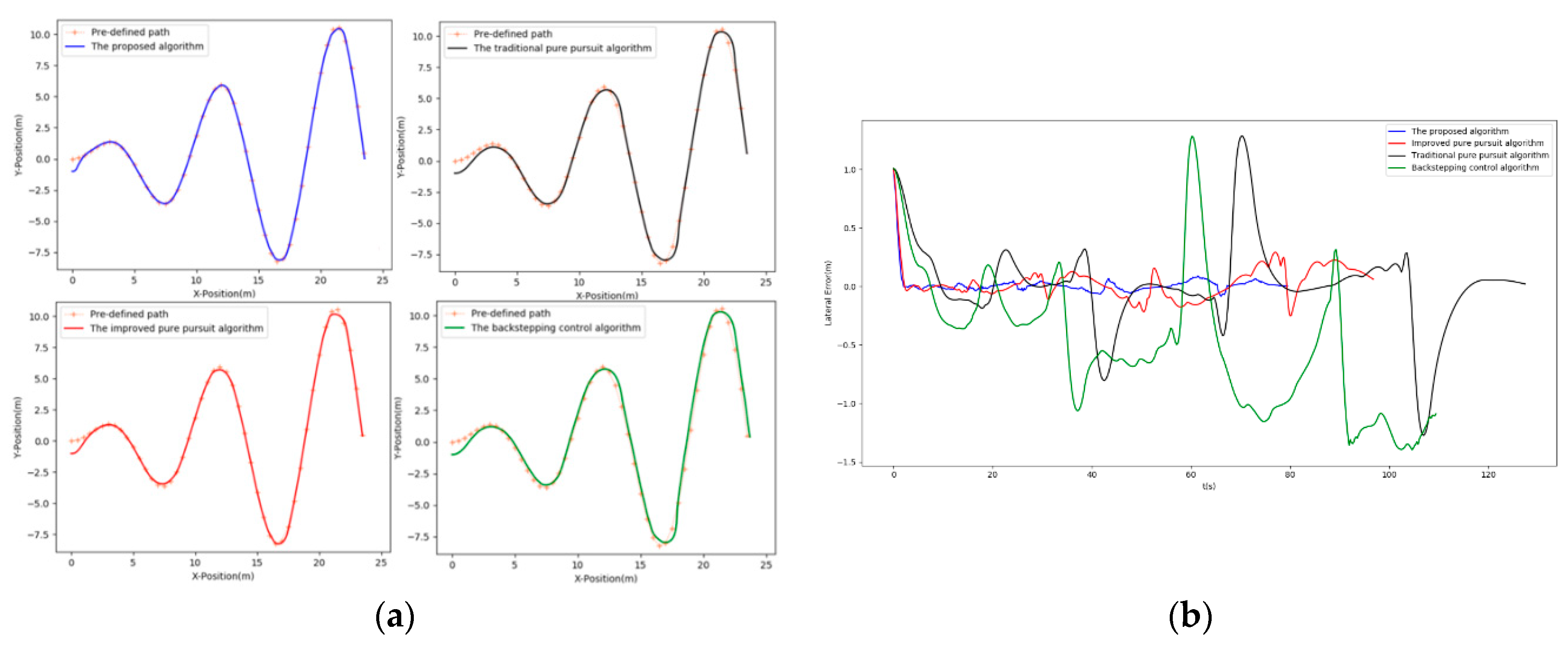
When tracking the path with multiple curvature, the simulation performance is shown in Figure 7a and lateral error is shown in Figure 7b. The chief reason for choosing this path is that the controller’s navigation ability can be tested in various turning operations. As can be seen from Figure 7a, the traditional pure pursuit algorithm can track the expected path after a period of oscillations in the initial stage, but the algorithm presented in this paper can quickly stabilize and show significant advantages. The errors of the traditional pure pursuit algorithm are large on the corners and the vehicle needs to be adjusted over and over again to track the expected path after turning. Although the improved pure pursuit algorithm expresses less deviation than the traditional pure pursuit algorithm at the turning points, it remains worse than the proposed algorithm. However, due to the existence of path curvature, the backstepping algorithm has the largest error in the tracking process. At corners, the proposed algorithm can adapt to the change of curvature quickly, and shows flexible adaptive ability to trace the expected path with tiny errors. In addition, the larger change rate of path curvature, the greater tracking errors of the four algorithms, but the proposed algorithm always performs a superior performance over other algorithms, and its maximum lateral error is 0.08 m after stabilization.

The above simulation results explain that the proposed method has better control performances and effects in ideal status without noise points. However, in order to verify the performance of this method, it is not enough without real vehicle experiments. Therefore, the field experimental result on a real cleaning vehicle are given below.

4.2. Field Experiment of Cleaning Vehicle

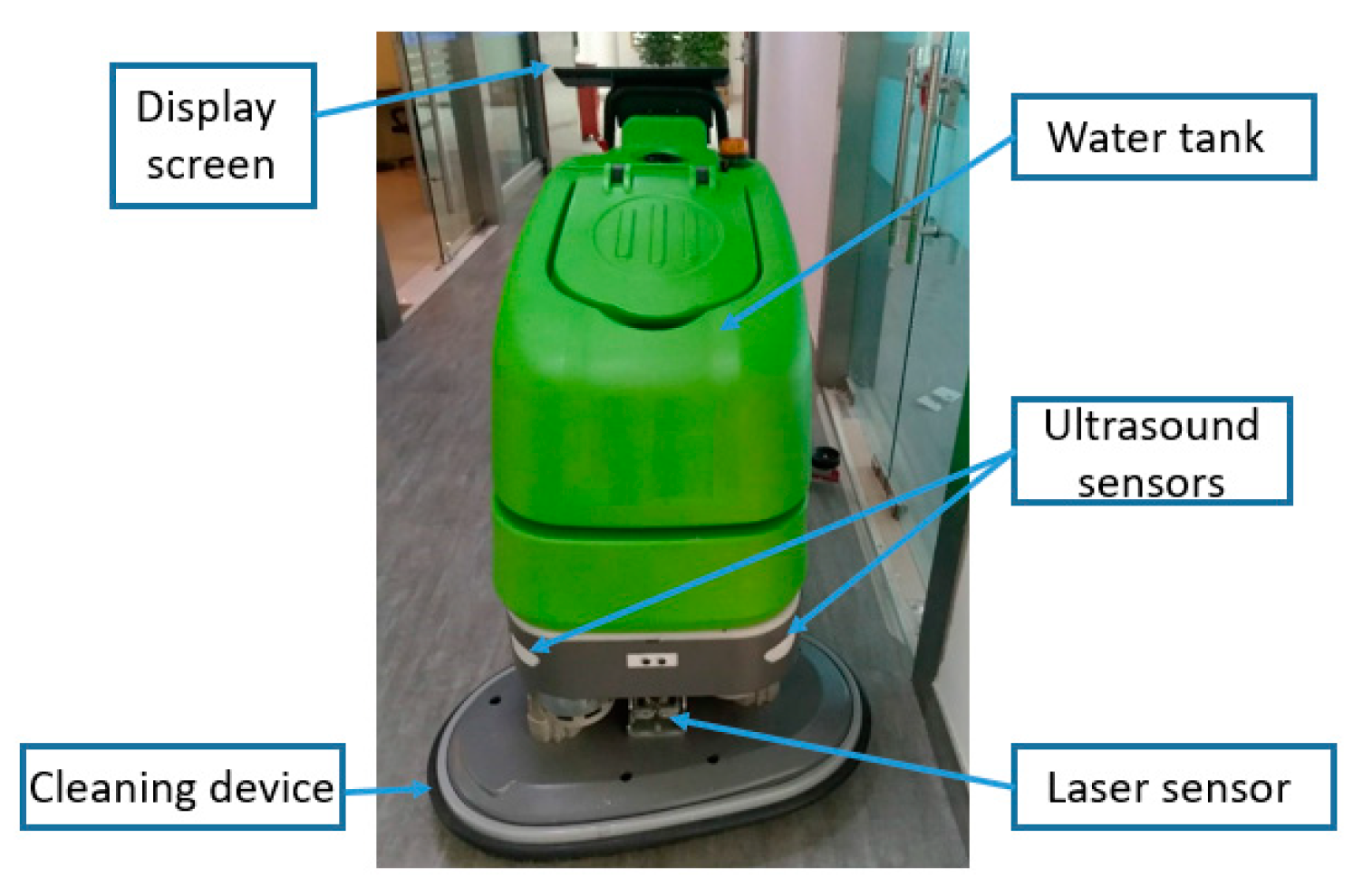
In order to test the actual working effect of this algorithm, the cleaning vehicle shown in Figure 8 is used in the field test. This cleaning vehicle is equipped with the laser radar and ultrasonic sensors. Its body length is 1.5 m and the wheelbase of two driving wheels is 1 m. There is a cleaning device in front of the vehicle and two driving wheels in the rear. Based on the practical experience and security factors, this machine is designed to have a speed of no more than 1 m/s.

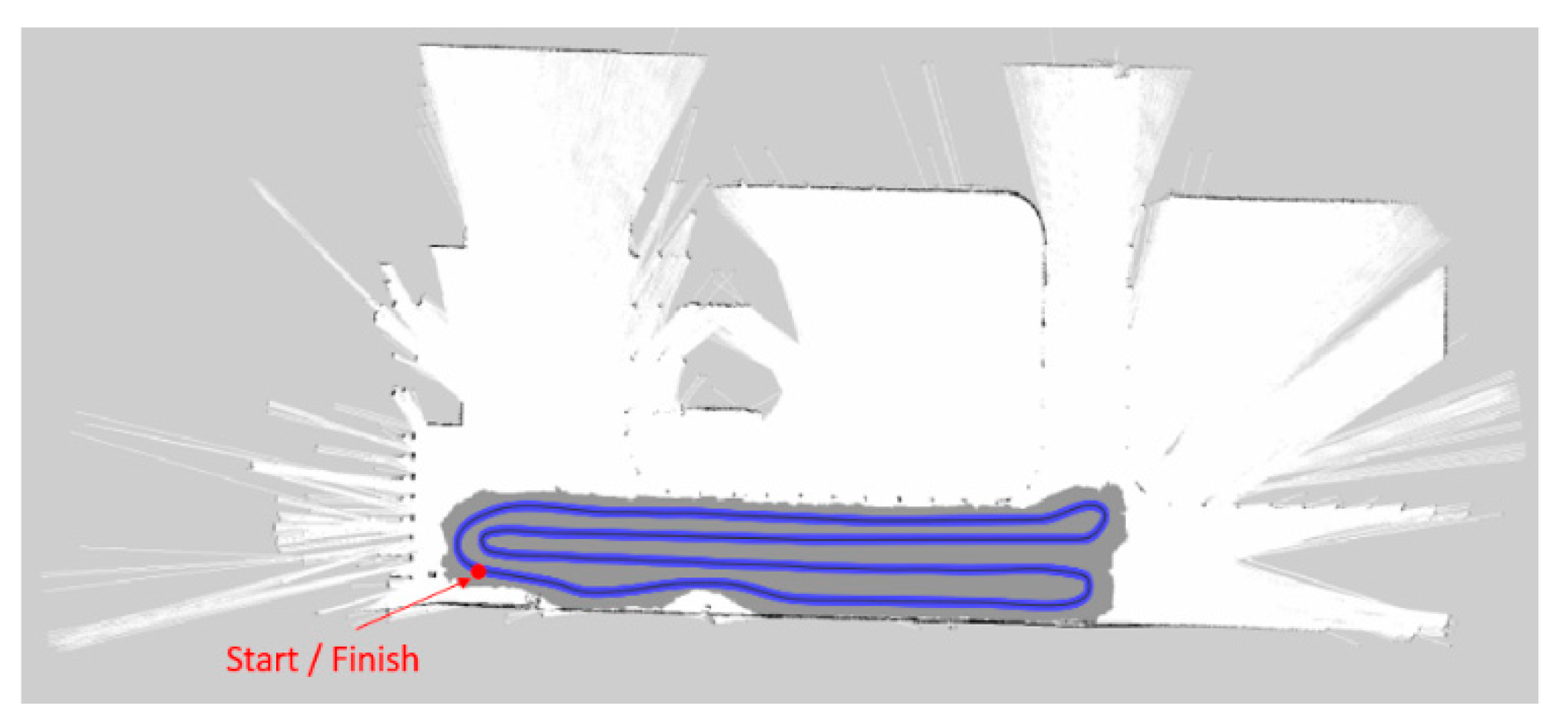
The field experiment is carried out in the subway station hall with the length of 30 m and the width of 3.8 m. It is necessary to manually specify the running route (pre-defined path) before the experiment by pushing the cleaning vehicle. The total length of running route is 197.3 m, the initial position of the vehicle is (0, 0), the initial yaw angle is 0°, and the initial speed is 0 m/s. The dark blue curve in Figure 9 is the specified running route.

In practice, an autonomous cleaning vehicle has to work on the paths with various shapes, so it needs a very robust tracking controller. Rapid changing path points require a re-computation of the speed and the yaw rate. Because the effect of traditional pure pursuit algorithm and backstepping algorithm control are often poor, these two methods are not tested in the field experiment.

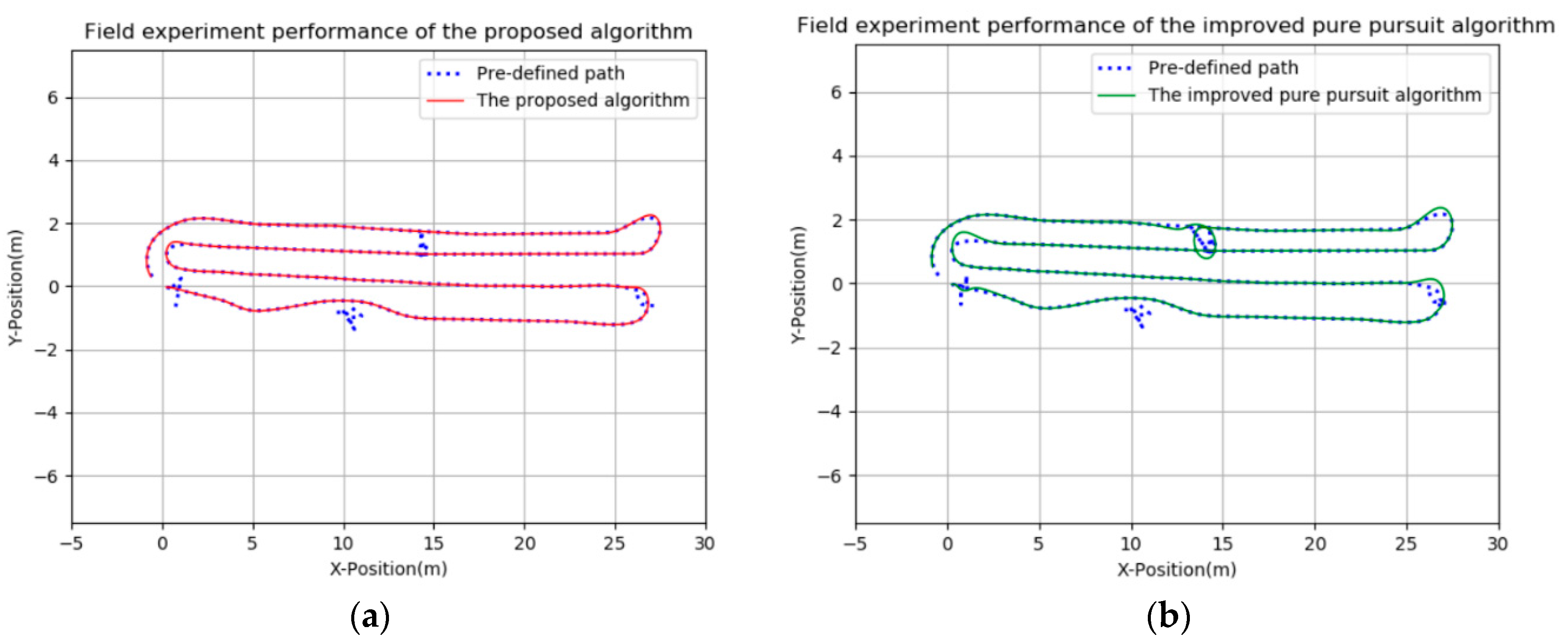
The target points tracking diagram is displayed in Figure 10, it can be seen that the proposed algorithm has more advantages than the improved pure pursuit algorithm, especially in the turning path and encountering the noise points. The proposed controller can track the reference path well in straight lines as well as corners, freedom from the impacts of noise points. However, the improved pure pursuit controller has large deviation at turning and it is easily disturbed by noise points. There may be a phenomenon that the cleaning vehicle does not follow the reference path when the noise point is too close to the real path. Besides, the cleaning vehicle can run or stop smoothly near the start point and the end point by adjusting the control parameters in Figure 10a. But in Figure 10b, noise points near the starting point affect the tracking process in the initial stage. In the final stage, the vehicle tracking ends ahead of schedule, because the preview distance and speed cannot be changed adaptively. Therefore, the field experimental results indicate that the proposed controller is robust and effective for the autonomous cleaning robot to track the pre-defined path points.

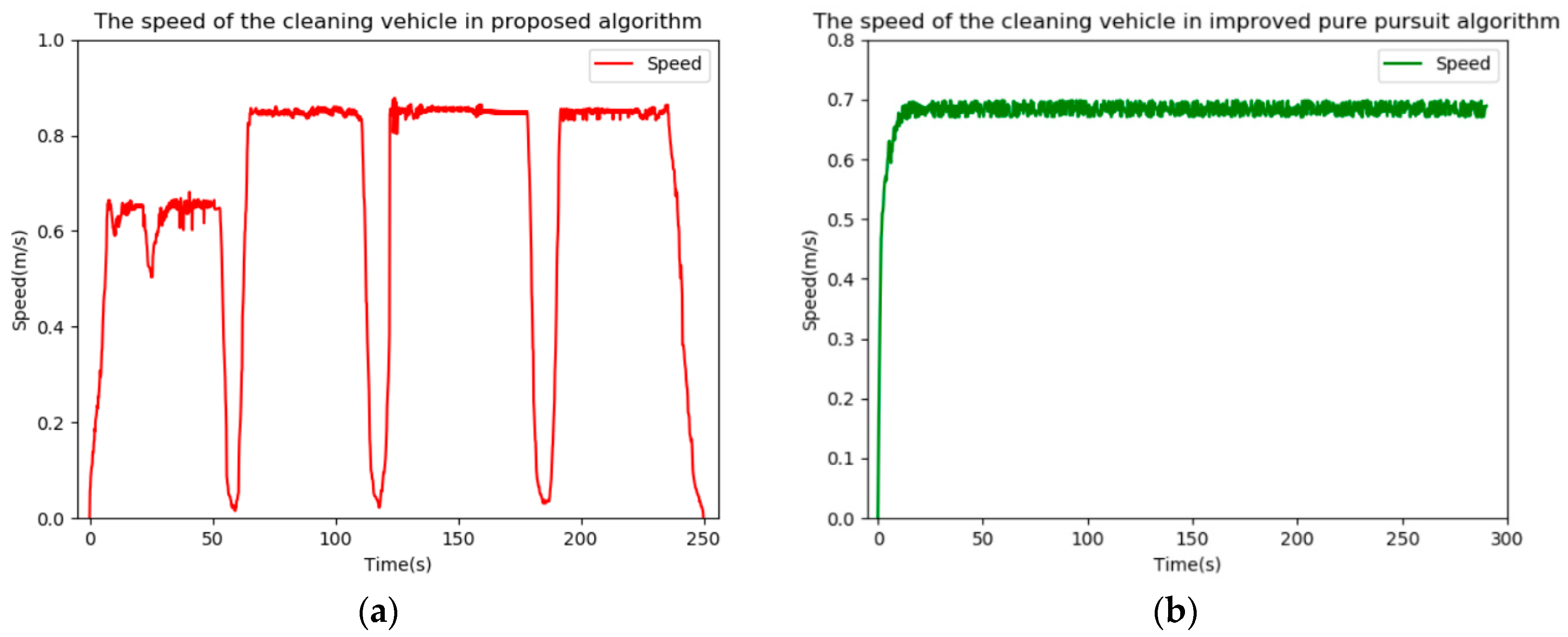
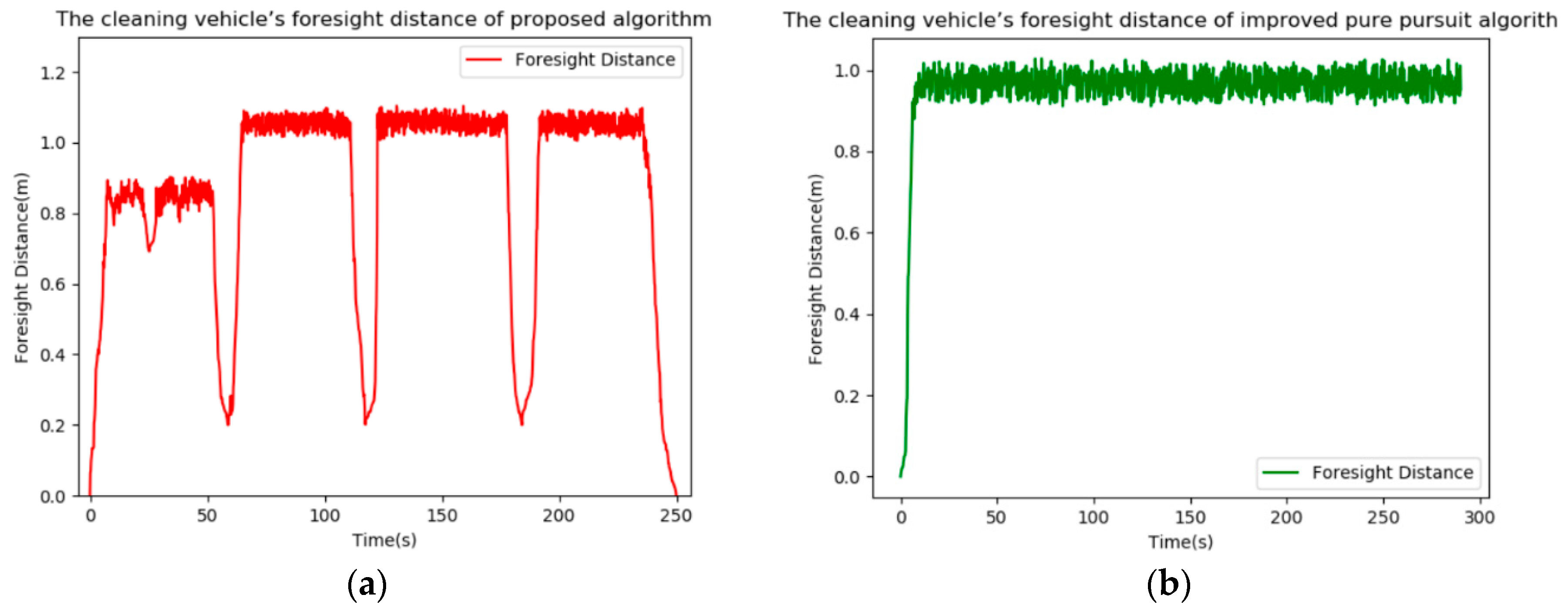
The Figure 11 and Figure 12 show the velocity and foresight distance variations of the two algorithms in tracking. The proposed controller is capable of adjusting the cleaning vehicle’s speed and the foresight distance intelligently. Throughout this process, these two values dropped observably on the corners. It is important to note that the LSTM network has learned the characteristics of the sample data. And the speed, as well as foresight distance when the vehicle walking against the wall (Saying that in approximately 0–50 s), are significantly less than the speed as well as foresight distance when not walking against the wall, except in the case of turning. However, in the improved pure pursuit algorithm, the speed and foresight distance increase slowly from 0 to the set values, but because the speed released by the controller may not be the same as the actual running speed of the vehicle, and vehicle needs to adjust the foresight distance according to the actual speed, so the speed and foresight distance have some vibration when the vehicle is in steady state. Unexpected speed and forward-looking distance are the reasons why the vehicle tracking ends early in the final phase.

The distance errors of target points tracking are obtained by comparing the reference path data with the tracking path data in automatic navigation. The average tracking error is 0.05 m, and the maximum tracking error is 0.13 m, which appears in the turning process of the cleaning vehicle. The average tracking error on the linear path is 0.02 m and the maximum tracking error is 0.04 m. These errors are within the allowable error range of the cleaning vehicle operation, which indicates that this algorithm has good navigation effect. During the cleaning process, the cleaning vehicle’s tracking route is accurate and reliable. Compared with the unintelligent speed vehicles, the intelligent changing speeds give the cleaning vehicle higher working efficiency.

5. Conclusions

Aiming at the influence of the foresight distance, driving speed and yaw rate for autonomous vehicles on the target point tracking control, a tracking controller based on the LSTM network is proposed in this paper. The foresight distance is obtained by the fuzzy control algorithm, whose inputs are the present velocity, yaw rate of the vehicle and output is an appropriate foresight distance. This distance is an important value with reference to the key parameter in pure pursuit algorithm. The two-layer LSTM network controller’s function is to regulate the autonomous vehicle’s speed and yaw rate simultaneously and intelligently to arrive at the target point, which is gained by a geometrical calculation based on the foresight distance. It is obvious that the foresight distance, driving velocity and yaw rate are interrelated. This method avoids the complicated process of traditional calculation and reduces the tracking error of point sequence tracking significantly.

The simulation experiments are carried out under the conditions of straight path as well as multiple curvature path, its results show that the proposed algorithm can adaptively adjust vehicle’s control parameters on the corners or straight segments to track different reference paths quickly and effectively. In order to verify the actual effectiveness of this algorithm, it is also applied to the tracking control of the cleaning vehicle in a subway station. The cleaning vehicle has a precise route and the swinging amplitude of the wheels is moderate during the running process in field experiment. Besides, the proposed controller is freedom from the impacts of path noise points, this phenomenon means that the proposed method can generate better speed and yaw rate for the path tracking in a broader field. Therefore, the proposed algorithm can not only reduce the labor costs, but also greatly improve the work efficiency and quality of the cleaning vehicle. It provides a reference for the research of target points tracking control of autonomous vehicles.