Article

Mitigation of Nonlinear Impairments by Using Support Vector Machine and Nonlinear Volterra Equalizer

Chair of Communications, Institute of Electrical Engineering and Information Technology, Kiel University, Kaiserstr. 2, 24143 Kiel, Germany
*
Author to whom correspondence should be addressed.
Appl. Sci. 2019, 9(18), 3800; https://doi.org/10.3390/app9183800
Submission received: 13 August 2019 / Revised: 2 September 2019 / Accepted: 4 September 2019 / Published: 11 September 2019
(This article belongs to the Special Issue Optics for AI and AI for Optics)

Abstract

:
A support vector machine (SVM) based detection is applied to different equalization schemes for a data center interconnect link using coherent 64 GBd 64-QAM over 100 km standard single mode fiber (SSMF). Without any prior knowledge or heuristic assumptions, the SVM is able to learn and capture the transmission characteristics from only a short training data set. We show that, with the use of suitable kernel functions, the SVM can create nonlinear decision thresholds and reduce the errors caused by nonlinear phase noise (NLPN), laser phase noise, I/Q imbalances and so forth. In order to apply the SVM to 64-QAM we introduce a binary coding SVM, which provides a binary multiclass classification with reduced complexity. We investigate the performance of this SVM and show how it can improve the bit-error rate (BER) of the entire system. After 100 km the fiber-induced nonlinear penalty is reduced by 2 dB at a BER of 3.7 × 10 3 . Furthermore, we apply a nonlinear Volterra equalizer (NLVE), which is based on the nonlinear Volterra theory, as another method for mitigating nonlinear effects. The combination of SVM and NLVE reduces the large computational complexity of the NLVE and allows more accurate compensation of nonlinear transmission impairments.

1. Introduction

The use of machine learning techniques in optical communication networks is currently a popular research topic [1]. Among the various algorithms for machine learning the support vector machine (SVM) can provide a powerful way of learning nonlinear functions. Besides noise, optical data transmission is also affected by linear and nonlinear impairments. Using coherent detection at the receiver, linear effects like chromatic dispersion can be successfully post-compensated by digital signal processing (DSP). Compensation can be done through a finite impulse response filter, also known as feed-forward equalizer (FFE). In case of long transmission distances, a separate electronic dispersion compensation (EDC) [2] is usually implemented, since otherwise too many coefficients for the adaptive FFE structure are required. With an increasing launch power, nonlinear effects additionally occur. For single-carrier transmission self-phase modulation (SPM), caused by the Kerr effect and nonlinear phase noise (NLPN), which results from the interaction between the amplified spontaneous emission (ASE) noise of inline optical amplifiers and SPM can be regarded as the most limiting nonlinear distortions [3]. These impairments cannot be compensated with conventional FFE structures. Previous approaches for the compensation of these nonlinear impairments focused on replacing the FFE by a nonlinear Volterra equalizer (NLVE) [4] or, if the fiber parameters are known, to replace the EDC with a digital backpropagation algorithm to compensate for linear and nonlinear effects simultaneously [5]. After using these methods, a signal detection with conventional linear decision thresholds takes place. Another approach for the compensation of nonlinear effects is an extended signal detection where the decision thresholds are adjusted to the disturbed constellations. In other words, the equalization problem is defined as a classification task. To solve this problem suitable algorithms such as expectation maximization (EM) [6,7], k-means algorithm (KMA) [8,9], neural network [10] or SVM [11] can be found in the large field of machine learning algorithms.
The advantage of extended signal detection by SVM is already emphasized in references [3,12,13,14]. In order to investigate exclusively the influence of nonlinearities such as NLPN or SPM, the influence of dispersion has been neglected deliberately in the past [3,12]. The absence of dispersion means that the interaction between dispersion and nonlinearities is not investigated. Thus, it should be examined whether these equalization techniques work equally well in dispersion influenced transmission.
In this paper we apply the SVM algorithm to a 64-QAM based coherent optical data center interconnect transmission system to mitigate nonlinear impairments after 100 km transmission distance, including the influence of dispersion. We numerically investigate, for the first time of our knowledge, the impact of different combinations of equalizer (FFE, NLVE) with various detection structures (SVM, KMA). Additionally, we show that the combination of SVM and NLVE can reduce the computational complexity of the NLVE and that this combination allows a more accurate compensation of the impairments that arise in an optical transmission system that is operated in the nonlinear regime.

2. Theoretical Analysis

2.1. Support Vector Machine

The support vector machine is a commonly used algorithm to classify data sets with binary output values. The method derived by Vladimir Vapnik is mainly based on the basics of statistical learning theory and applies the quadratic optimization problem to distinguish two classes in a feature space [15]. The training is done with a training set S of length N and consists of the input data x i and binary classified data y i :
S = ( x 1 , y 1 ) , , ( x n , y n ) , x i R n , y i ± 1
In order to separate the input features, a hyperplane h ( x ) is calculated by a quadratic optimization problem. To allow more general decision surfaces, the input data is mapped to a higher dimensional feature space, that is, ϕ ( x ) R m , where the data is linearly separable. The SVM classifies an estimation according to
y ^ = sign { w T ϕ ( x ) + b } ,
where w and b are an orthogonal vector to h ( x ) and a bias term, respectively, which are determined in a training process. The optimal hyperplane is found, if the margin—smallest distance between the hyperplane and any of the samples—is maximized [3,16].
The mentioned optimization problem distinguishes two classes whose feature vectors are located in an ideally delimitable area. If there are strong deviations of individual data points in the training set, for example, if a data point is located in the area of the contrary class, it is not possible to separate the data successfully. The problem can be solved by using a soft margin classifier. This enables a tolerance against data anomalies. For this purpose the optimization problem is extended by an error term including a weighting coefficient C and slack variables ξ [3]
min w , b , ξ 1 2 | | w | | 2 + C i = 0 N ξ i
under constraints
y i ( w T ϕ ( x ) + b 1 ξ i )
ξ i 0 , i = 1 , , N .
The basic algorithm of the SVM has been formulated in terms of scalar products in the feature space F. According to Mercer’s theorem the intensive calculation in the higher dimensional space can be significantly reduced by a suitable kernel function K ( x , x i ) = ϕ ( x ) · ϕ ( x i ) [16]. With the use of different kernels, diverse problems can be solved, which opens up a wide variety of SVM learning machines. In case of M-QAM transmission, the radial base function (RBF) is the most suitable kernel and is defined by
K ( x , x i ) = exp ( γ | | x x i | | 2 )
with the kernel parameter γ > 0 [16].

SVM-based Detection

For coherent optical communications systems, the modulation format M-QAM is usually selected. To be able to process the signals at the receiver by using an SVM, each cluster of the signal constellation represents one class, for example, 16-QAM consists of 16 classes. Since the SVM is fundamentally a binary classifier, an extension of the SVM structure is required. Various methods have been proposed for combining multiple binary SVMs in order to build a multi-class SVM. Common methods to extend the SVM are the one-vs-one (OVO), one-vs-all (OVA) and binary-coding SVM (BCSVM) or also called M-ary SVM [15]. The OVO principle is based on the comparison of two different classes from the entire set of all classes. If a data set contains N different classes, then N ( N 1 ) / 2 different binary SVMs are trained. For the concluding decision a voting procedure is used and the class with the highest vote is detected. In the OVA scheme the data of one class is separated from the complete data of all remaining N 1 classes. Thus, N SVMs are trained. At the end, the class with the highest vote is detected. For communication systems, the BCSVM is the most appropriate choice. The symbols or classes are already labelled in binary format, enabling each individual bit to be modelled with one conventional SVM. For M-QAM log 2 ( M ) SVMs are required.
Figure 1a shows the principle of the BCSVM for 16-QAM. The respective SVMs are color-coded with the corresponding bits. Figure 1b illustrates the processing structure. The complex input vector x rx contains the received symbols divided into real and imaginary parts. Training is done according to the transmitted bit sequence y . The separating hyperplane of each SVM is determined by quadratic programming during training [3].
The output of the binary SVM array is an estimation of the transmitted bit sequence y ^ = [ y ^ 1 , y ^ 2 , y ^ 3 , y ^ 4 ] . Consequently, the received signal is classified and demodulated at the same time.
Figure 2 exemplarily shows an iteration of the training process of the presented methods. The data points of the two opposite classes are colored red or blue. It can be seen, that the OVA and BCSVM method, in contrast to the OVO, take into account all data points in each iteration step. This may result in a significant computational complexity, if too much training data is used. However, the OVO method requires significantly more iterations steps than the other methods [17].
During the training process it is necessary to adapt certain parameters of the optimization problem to the characteristics of the input data. The aim is to avoid over- or underfitted systems, which leads to a significantly reduced classification accuracy [12]. The adaptation and verification is implemented using the two optimization algorithms Grid-Search and Cross Validation [12,18]. In the optimization process, 70% of the training data is used for training and 30% for validation.

2.2. Nonlinear Volterra Equalizer

The principle of the NLVE is based on the theory of the Volterra series, which is an important tool for the analysis of nonlinear systems and provides a complete description of the channel nonlinearity [19,20]. The realization can be done either in the frequency domain or entirely in the time domain, as will be shown here. A general discrete Volterra filter input-output relation is given by [4]
y n = v = 0 N 1 1 e v x n v + v = 0 N 2 1 l = v N 2 1 e v , l x n v x n l + v = 0 N 3 1 l = v N 3 1 m = 0 N 3 1 e v , l , m x n v x n l x n m * ,
where x n and y n are the complex-valued filter input and output of the equalizer at the time index n, N i is the memory length of the i-th order and e v , e v , l , e v , l , m are the equalizer coefficients. The first term of Equation (7) represents a linear filter, whereas the others are nonlinear.
The coefficients can be estimated using the minimum mean square error (MMSE) criterion. The dimension of the model grows rapidly, as can be seen from the total number of coefficients given by
N t = N 1 + N 2 ( N 2 + 1 ) / 2 + N 3 2 ( N 3 + 1 ) / 2 .
According to Equation (7) we choose the notation NLVE[ N 1 , N 2 , N 3 ] as full description of the Volterra filter. In this case N 1 - N 3 represents the memory length of the 1st–3rd order of the NLVE.

3. Simulation Setup

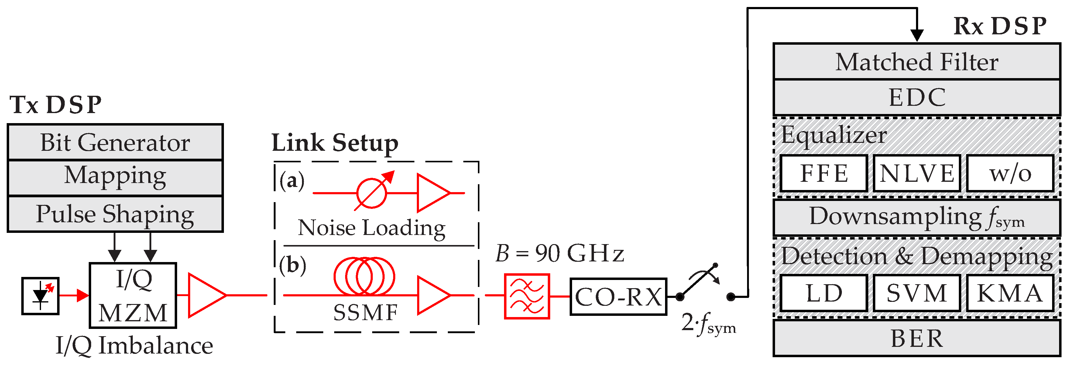
The proposed techniques are subsequently thoroughly evaluated in numerical simulations for a 64 GBd 64-QAM system. For simulation purposes we will initially restrict ourselves to a single-polarization system but it can be extended straight forward to a dual-polarization system. A schematic of the general setup is given in Figure 3. A 2 16 randomly generated bit sequence, using the MATLAB R2018a (9.4.0.813654) rand function, is mapped to the 64-QAM symbols. The digital to analog conversion is modelled as a root-raised cosine pulse shaping filter with roll-off factor β = 0.3 . The symbols are modulated on the carrier (wavelength λ c = 1550 nm) via an I/Q MZ-modulator. The linewidth of the laser is set to zero. The modulated optical signal is coupled into the fiber after it is amplified by the erbium doped fiber amplifier (EDFA) with a noise figure (NF) of 5 dB.
In order to investigate the performance of the enhanced detection algorithms, two types of communication systems are modeled. The link setup (a) is used to test a back-to-back (B2B) scenario, that is, no transmission link was simulated. The setup (b) is used to examine a dispersion uncompensated link, where the dispersion is compensated by DSP at the end of the transmission. The parameters for the SSMF are given by the attenuation coefficient α = 0.2 dB/km, the dispersion coefficient D = 17 ps/(nm·km), dispersion slope S = 0.06 ps/(nm 2 ·km) and the nonlinear coefficient γ = 1.3 (W·km) 1 . For a complete compensation of span loss an EDFA (NF = 5 dB) is applied. After transmission a Gaussian optical filter with 90 GHz bandwidth is used to reduce ASE noise. The received signal is detected by a coherent receiver and downsampled to 128 GS/s. After matched filtering an ideal EDC is used to compensate for dispersion. After the equalization stage, which consists of either an FFE, an NLVE or no equalizer at all (w/o), the signal is downsampled to symbol frequency and detected. Detection and demodulation is performed either linear by using conventional linear decision thresholds and demapping, here called linear detection (LD), or by machine learning algorithms such as SVM or KMA [8,9]. System performance is evaluated by BER. The hard-decision forward error correction (HD-FEC) limit is assumed to be 3.7 × 10 3 . We examine the suitability of the SVM as a classifier and combine the mentioned equalizer schemes with the SVM to achieve the maximum gain of the machine learning algorithm.
Since more coefficients require more training symbols, increasing the number of coefficients without adjusting the number of training symbols might decrease the performance. Thus, for a correct adjustment of the Volterra equalizer it is necessary to determine the optimal number of coefficients and training symbols. For the further investigations the training length of 2048 symbols and memory lengths of NLVE[4,2,5] was determined after optimization.

4. Results and Discussion

Initially the behavior of SVM against I/Q imbalances was examined. In an I/Q modulator, the ideal phase shift between the I- and Q-branch is 90°. Due to physical imperfections of the system components and the non-perfect tuning of the π /2 phase shift, amplitudes and phase mismatches may occur. These I/Q imbalances may considerably disturb the signal constellation [21]. We investigate the I/Q imbalances in a B2B scenario according to 
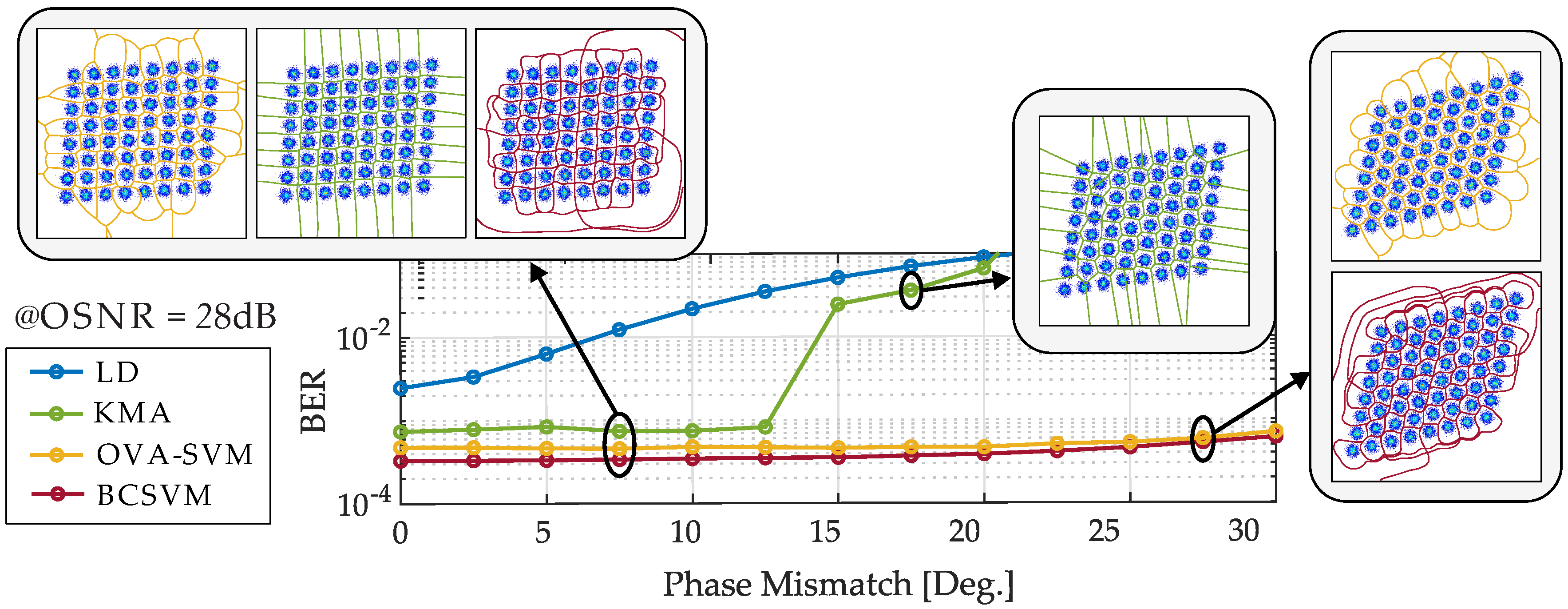
Figure 3a at an optical signal-to-noise ratio (OSNR) of 28 dB, where the signal is disturbed at the transmitter side. The amplitude mismatch is set to 0.125 and the phase mismatch is varied between 0° and 30°. To cope with these imperfections, we examine the performance of the BCSVM and the OVA-SVM and compare them to LD. In order to compare the SVM with other enhanced detection techniques, the KMA is added to this comparison. The training length of the respective SVMs and KMA is set to 1024 symbols. Moreover, the number of iterations for KMA is set to 5.
Figure 4 shows the performance of the various detection methods depending on the transmitter I/Q imbalances. As expected, detection by machine learning algorithms is more robust against I/Q imbalances compared to LD. For low phase mismatch, the performance of the two enhanced detection techniques seems similar. However, above 12° phase mismatch the KMA’s performance rapidly deteriorates. For SVM a decline in performance can be observed above 20° phase mismatch. Compared with OVA-SVM, the BCSM achieves slightly better performance, which is in the range of 1 × 10 4 .
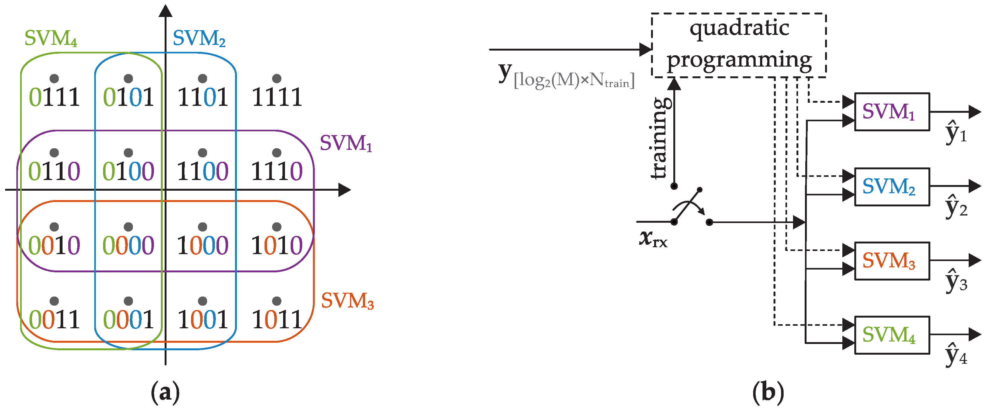
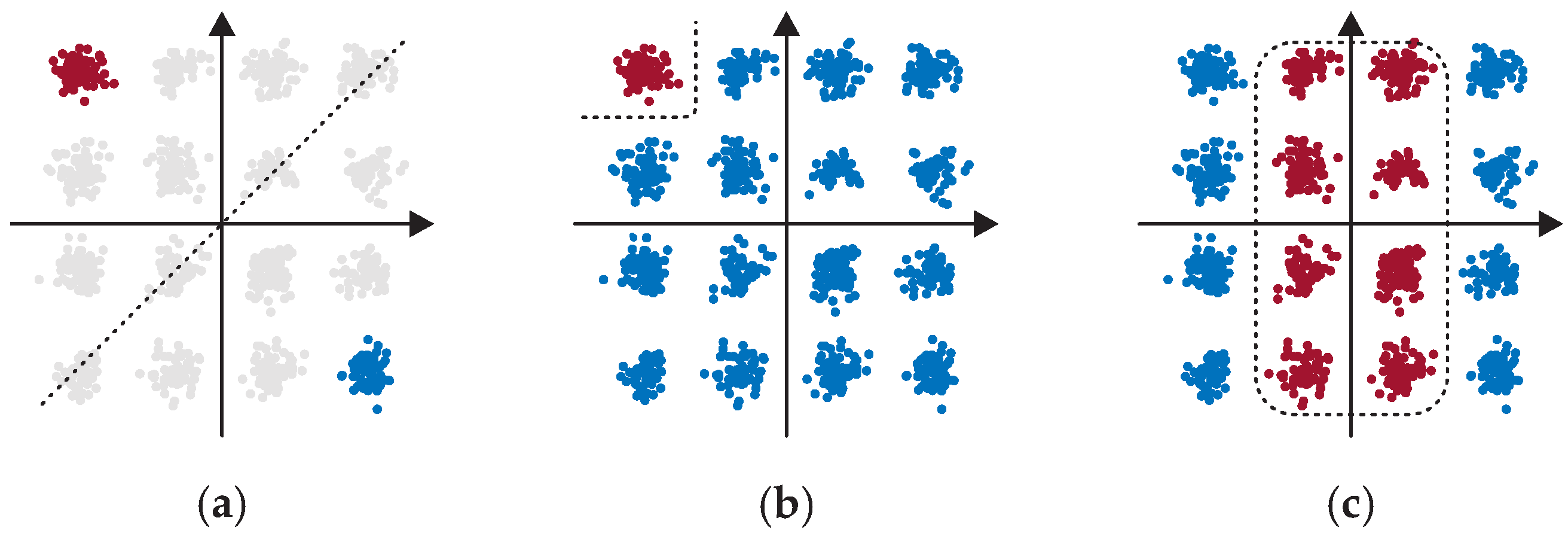
It should be mentioned that SVM and KMA are two completely different procedures. The SVM has already been introduced as classification algorithm in Section 2.1. The KMA, in contrast, belongs to a cluster-based detection. The training of KMA is iterative and unsupervised, while the training of the SVM is supervised. The KMA is initialized with the centers of the cluster. Therefore, it is necessary to know how many clusters are present and where the centers are approximately expected. If the actual cluster is too far away from the expected cluster, the KMA is no longer able to separate the clusters correctly. This can be seen for example in the constellation of the KMA at 17.5° phase mismatch, where the field at the top right has been assigned to about two full constellation points. Although the centers of the clusters are updated in each iteration. This effect may also occur in case of a phase rotation induced by SPM. Furthermore, the KMA is only a linear algorithm in essence, while the SVM is a nonlinear classifier due to the usage of kernels. Accordingly, the KMA is unsuitable for highly complex and nonlinear data distributions and is therefore no longer used as comparison in the following investigations.
Regarding the visualization of the decision thresholds, the different working principles of the algorithms can be observed. Based on the RBF kernel, the SVM calculates significantly rounder and softer decision thresholds than the KMA. Additionally, a difference between the multi-class methods of the SVM can be seen. Therefore, we would like to point out at this point that besides the selection of the kernel also the choice of the SVM multi-class method may have a more or less significant influence on the results.
Next, we include the fiber in our simulations. To evaluate the ability of the SVM to compensate nonlinear impairments in the 100 km setup for different launch powers, we compare the nonlinear detection by SVM with an FFE and an NLVE. To distort the 64-QAM constellation we set the modulation depth of the modulator to m = V pp / V π = 2.2 and generated an I/Q imbalance with 5% phase deviation from 90°. The number of training symbols for SVM is set to 1024.
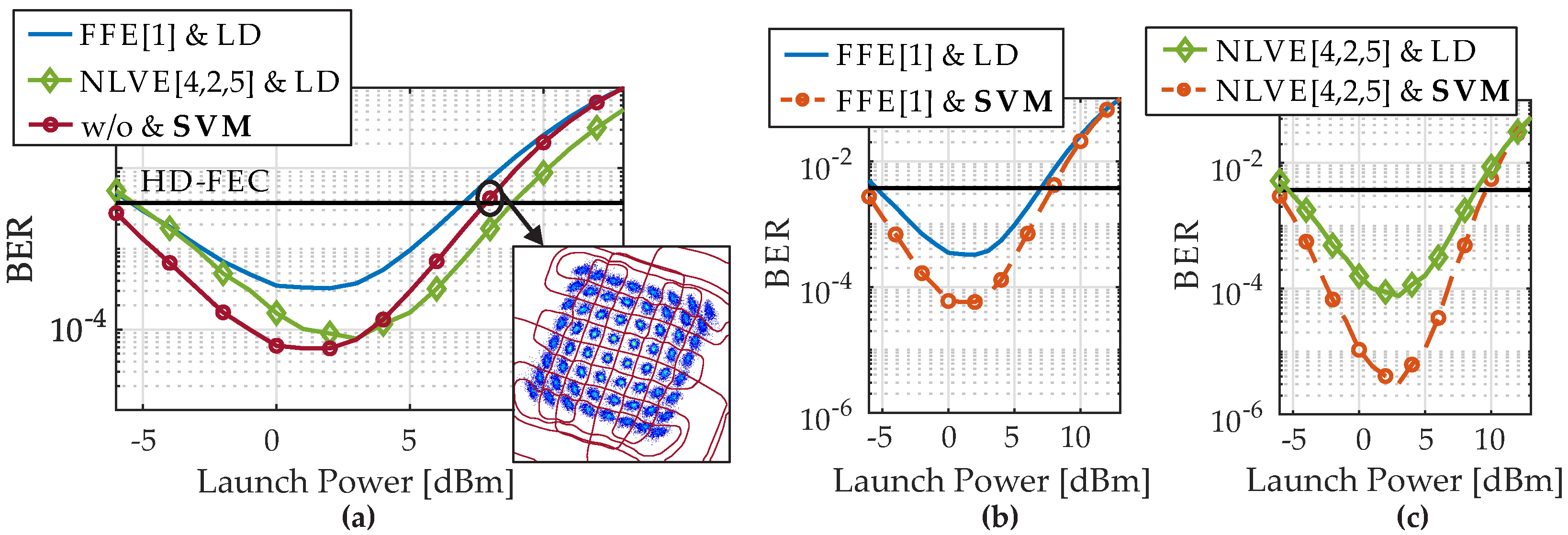
The BER as a function of the launch power after 100 km dispersion uncompensated transmission is shown in Figure 5. The launch power of the 64-QAM signal ranges from −6 to +12 dBm. We investigate different combinations of equalizers and detection techniques. Figure 5a first presents the results for FFE[1] and NLVE[4,2,5] in conjunction with LD. In addition, the red curve shows a detection based on SVM only without any previously inserted equalizer. It can be seen that a nonlinear detection with SVM only is already quite powerful. Here, the lowest BER is achieved by SVM at 3 dBm launch power, which is about six times lower than the BER using the FFE. Up to 4 dBm the best results can be achieved with SVM detection. Above 4 dBm nonlinear effects dominate and the optimally configured NLVE shows the best performance while the SVM is not as good as the NLVE but still better than the FFE. The launch power to stay below HD-FEC can be increased by 2 dB, if NLVE[4,2,5] is used and by 1 dB if the SVM is used compared to FFE[1]. If an FFE[1] or NLVE[4,2,5] is now added before the SVM, the overall system performance can be improved significantly, as shown in Figure 5b,c. Especially the combination of NLVE[4,2,5] and SVM further minimizes the BER significantly as can be seen in Figure 5c at 3 dBm launch power, where the BER is reduced from 7.7 × 10 5 to 3.1 × 10 6 by SVM.
The optimum setting for the NLVE is given by NLVE[4,2,5]. So, the total number of NLVE coefficients sums up to N t = 82 , according to Equation (8). The majority of coefficients belongs to the third order of the NLVE. Therefore, in our further investigations we have reduced the number of delay elements in the third order to N 3 = 3 . Consequently, the number of coefficients is decreased from 75 to 18 (74%). Figure 6 shows the obtained BER as a function of the launch power for the optimal and reduced NLVE. The SVM is trained with 1024 and the NLVE with 2048 symbols. It can be seen that further reducing the coefficients of the NLVE leads to a decline of the overall system performance. To stay below the HD-FEC, the launch power is reduced by 1 dB in case of NLVE[3,2,3] and LD compared to the NLVE[4,2,5] and LD. Furthermore, NLVE[4,2,3] is continuously worse than a detection by SVM only. By combining the reduced NLVE[4,2,3] and the SVM, it can be observed that better results are achieved compared to the optimally adjusted NLVE[4,2,5] and LD. At 3 dBm launch power, the BER of NLVE[4,2,3] and LD (green dashed line) is 1.2 × 10 4 and can be reduced to 1 × 10 5 by SVM (orange dashed line).
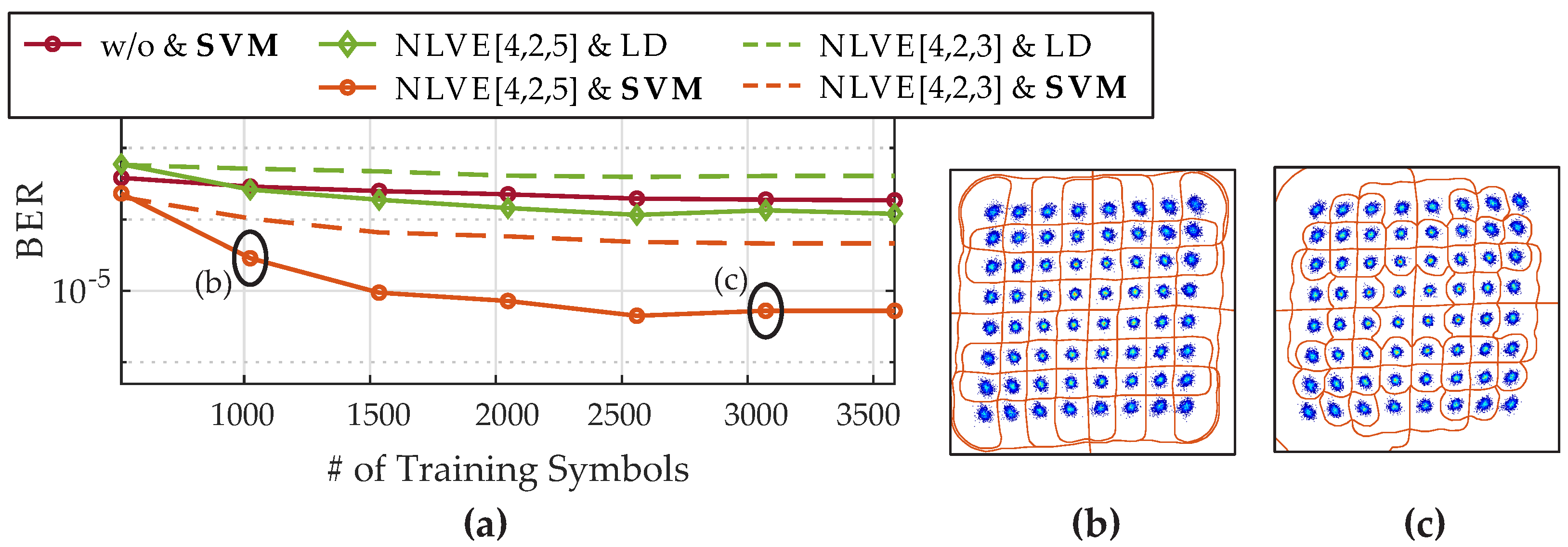
Finally, we examined the impact of the number of training symbols on the performance of the NLVE and the SVM. The obtained results are presented in Figure 7 including the investigations for the NLVE with optimal and reduced coefficients in combination with LD and SVM based nonlinear detection plus a single detection only by SVM. We increased the number of training symbols from 512 to 3584 at 5 dBm launch power. The main improvement is observed after an increase from 512 to 1024 symbols for all investigated structures.
The training of the SVM is based on the classes that are included in the classification task. To ensure that the SVM can learn and capture link properties from ony a small amount of training data [12], it is important, that besides a sufficient number of training symbols all classes are uniformly distributed in the training set. For example, with the amount of 512 training symbols and 64 different classes it is not guaranteed that each class is included in the training data, if a randomly generated training sequence is used. Concerning the NLVE, the training is based on the amount of inter symbol interference which is independent on the training data itself. Here, a certain number of symbols is necessary to estimate the coefficients correctly. In case of the NLVE[4,2,5], the training length of 512 is not sufficient to determine the coefficients correctly. However, if a certain number of training symbols is used, the channel estimation of the NLVE can improve its performance barely, even if more training data is used as it can be seen for the reduced NLVE[4,2,3]. While the plain NLVE and SVM structures saturated fast, the results with combined NLVE and SVM based detection are quite remarkable.

5. Conclusions

In this paper we compared and combined nonlinear detection by SVM with post-compensation techniques for the mitigation of nonlinearities regarding their performance and computational complexity. Unlike clustering and classification algorithms like EM or KMA, the SVM does not require any prior knowledge of the modulation format. We have shown that by combining NLVE and SVM based detection it is possible to improve the overall system performance for 64 GBd 64-QAM coherent transmission over 100 km. For example, at 3 dBm launch power, the BER is reduced from 7.7 × 10 5 to 3.1 × 10 6 by SVM. It is well known that nonlinear equalization using an NLVE is computationally quite complex, so a trade-off between complexity and performance is often required. Therefore, the performance of a reduced NLVE was evaluated and the obtained results have shown, that by adding an SVM it is possible to reduce the number of coefficients by 74% while maintaining or improving the overall system performance. The SVM classification approach provides a way to cluster datasets without prior knowledge of the channel characteristics or the modulation format. Based on the previous studies and discussions, we strongly believe that in context of coherent optical transmission systems, an enhanced detection by using SVM and its methods should be further investigated. So far, we mainly examined a single channel and single-polarization. Other effects among multiple channels and polarization effects will be taken into account in future studies.

Author Contributions

Conceptualization, R.W., J.K., P.P. and S.P. developed the concept; formal analysis, R.W. and J.K.; designed and performed the simulations and analyzed the data; writing—original draft preparation, R.W. and P.P.; writing—review and editing, J.K., S.O. and S.P.

Funding

This research received no external funding.

Acknowledgments

We gratefully acknowledge the support of NVIDIA Coorporation for the donation of the Titan Xp GPU used for this research.

Conflicts of Interest

The authors declare no conflict of interest.

Abbreviations

The following abbreviations are used in this manuscript:
ASEAmplified Spontaneous Emission
BCSVMBinary Coding Support Vector Machine
BERBit Error Ratio
B2BBack-to-Back
DSPDigital Signal Processing
EDCElectronic Dispersion Compensation
EDFAErbium Doped Fiber Amplifier
HD-FECHard-Decision Forward Error Correction
KMAK-Means Algorithm
LDLinear Detection
MMSEMinimum Mean Square Error
NFNoise Figure
NLPNNonlinear Phase Noise
OVAOne versus All
OVOOne versus One
OSNROptical Signal-to-Noise Ratio
QAMQuadrature Amplitude Modulation
RBFRadial Basis Function
SSMFStandard Single Mode Fiber
SVMSupport Vector Machine

References

  1. Musumeci, F. An overview on application of machine learning techniques in optical networks. IEEE Commun. Surv. Tutor. 2018, 21, 1383–1408. [Google Scholar] [CrossRef]
  2. Bülow, H.; Buchali, F.; Klekamp, K. Electronic Dispersion Compensation. J. Light. Technol. 2008, 26, 158–167. [Google Scholar] [CrossRef]
  3. Li, M.; Yu, S.; Yang, J.; Chen, Z.; Han, Y.; Gu, W. Nonparameter nonlinear phase noise mitigation by using M-ary support vector machine for coherent optical systems. IEEE Photonics J. 2013, 5, 7800312. [Google Scholar] [CrossRef]
  4. Han, X.; Chen, C. Nonlinear filter based decision feedback equalizer for optical communication systems. Opt. Express 2014, 22, 8712–8719. [Google Scholar] [CrossRef] [PubMed]
  5. Ip, E.; Kahn, J.M. Compensation of dispersion and nonlinear impairments using digital backpropagation. J. Light. Technol. 2008, 262, 3416–3425. [Google Scholar] [CrossRef]
  6. Moon, T.K. The expectation-maximization algorithm. IEEE Signal Process. Mag. 1996, 13, 47–60. [Google Scholar] [CrossRef]
  7. Zibar, D.; Winther, O.; Franceschi, N.; Borkowski, R.; Caballero, A.; Arlunno, V.; Schmidt, M.; Gonzales, N.; Mao, B.; Ye, Y.; et al. Nonlinear impairment compensation using expectation maximization for dispersion managed and unmanaged PDM 16-QAM transmission. Opt. Express 2012, 20, B181–B196. [Google Scholar] [CrossRef] [Green Version]
  8. Aggarwal, C.C. A human-computer interactive method for projected clustering. IEEE Trans. Knowl. Data Eng. 2004, 16, 448–460. [Google Scholar] [CrossRef]
  9. Dong, J.; Qi, M. K-means optimization algorithm for solving clustering problem. In Proceedings of the 2009 Second International Workshop on Knowledge Discovery and Data Mining, Moscow, Russia, 23–25 January 2009; pp. 52–55. [Google Scholar]
  10. Chuang, C.-Y.; Liu, L.-C.; Wei, C.-C.; Liu, J.-J.; Henrickson, L.; Huang, W.-J.; Wang, C.-L.; Chen, Y.-K.; Chen, J. Convolutional neural network based nonlinear classifier for 112-Gbps high speed optical link. In Proceedings of the Optical Fiber Communications Conference (OFC), San Diego, CA, USA, 11–15 March 2018. [Google Scholar]
  11. Bishop, C.M. Sparse kernel machines. In Pattern Recognition and Machine Learning; Springer: Berlin/Heidelberg, Germany, 2006; pp. 352–359. [Google Scholar]
  12. Wang, D.; Zhang, M.; Cai, Z.; Cui, Y.; Li, Z.; Han, H.; Fu, M.; Luo, B. Combatting nonlinear phase noise in coherent optical systems with an optimized decision processor based on machine learning. Opt. Commun. 2016, 369, 199–208. [Google Scholar] [CrossRef]
  13. Han, Y.; Yu, S.; Li, M.; Yan, J.; Gu, W. An SVM-based detection for coherent optical APSK systems with nonlinear phase noise. IEEE Photonics J. 2014, 6, 1–10. [Google Scholar] [CrossRef]
  14. Lau, A.P.T.; Kahn, J.M. Signal design and detection in presence of nonlinear phase noise. J. Light. Technol. 2007, 25, 3008–3016. [Google Scholar] [CrossRef]
  15. Sebald, D.J.; Bucklew, J.A. Support vector machines and the multiple hypothesis test problem. IEEE Trans. Signal Process. 2001, 49, 2865–2872. [Google Scholar] [CrossRef]
  16. Schölkopf, B. Support Vector Learning; Technical University of Berlin: Berlin, Germany, 1997. [Google Scholar]
  17. Zhibin, L.; Lianwen, J. LATTICESVM—A new method for multi-class Support Vector machines. In Proceedings of the 2008 IEEE International Joint Conference on Neural Networks (IEEE World Congress on Computational Intelligence), Hong Kong, China, 1–8 June 2008; pp. 727–733. [Google Scholar]
  18. Hsu, C.-W.; Chang, C.-C.; Lin, C.-J. A practical guide to support vector classification. BJU Int. 2003, 101, 1396–1400. [Google Scholar]
  19. Gao, Y.; Zhang, F.; Dou, L.; Chen, Z.; Xu, A. Intra-channel nonlinearities mitigation in pseudo-linear coherent QPSK transmission systems via nonlinear electrical equalizer. Opt. Commun. 2009, 282, 2421–2425. [Google Scholar] [CrossRef]
  20. Peddanarappagari, K.V.; Brandt-Pearce, M. Volterra series transfer function of single-mode fibers. J. Light. Technol. 1997, 15, 2232–2241. [Google Scholar] [CrossRef]
  21. Petrou, C.; Vgenis, A.; Roudas, I.; Raptis, L. Quadrature imbalance compensation algorithms for coherent PDM QPSK systems. IEEE Photonics Technol. Lett. 2009, 21, 1876–1878. [Google Scholar] [CrossRef]
Figure 1. Binary Coding Support Vector Machine (BCSVM) nonlinear classification using four support vector machines (SVMs) [3]: (a) Coding and classification scheme for BCSVM based detection and (b) the processing structure for BCSVM used for 16-QAM signal detection.
Applsci 09 03800 g001
Figure 2. Illustration of one iteration during training for (a) OVO, (b) OVA and (c) BCSVM methods in case of 16-QAM transmission. The opposite classes are marked in red and blue and the corresponding hyperplane is indicated by the dashed line.
Applsci 09 03800 g002
Figure 3. Simulation setup of the 64 Gbd 64-QAM single-polarization coherent optical simulation system including two different setups for the link. By using the setup (a) a B2B transmission with noise loading is examined. The setup (b) consists of a 100 km SSMF transmission with subsequent electronic dispersion compensation (EDC) to investigate a dispersion uncompensated link.
Applsci 09 03800 g003
Figure 4. Simulations results in case of transmitter I/Q imbalances. BER vs. phase mismatch for an amplitude mismatch of 0.125 and 28 dB OSNR.
Applsci 09 03800 g004
Figure 5. BER as a function of the launch power at 100 km dispersion unmanaged transmission: (a) shows equalization by FFE[1] and NLVE[4,2,5] combined with LD and only SVM detection. (b) shows the combined structure FFE[1] and SVM and (c) shows the combination NLVE[4,2,5] with SVM.
Applsci 09 03800 g005
Figure 6. BER as a function of the launch power at 100 km for NLVE equalization with optimal and reduced number of coefficients in combination with SVM based detection.
Applsci 09 03800 g006
Figure 7. (a) Shows the BER as function of the number of training symbols for 100 km dispersion unmanaged transmission at 5 dBm launch power. (b) Shows the the corresponding constellation diagram for NLVE[4,2,5] & SVM trained with 1024 symbols and (c) Shows the constellation diagram for NLVE[4,2,5] & SVM trained with 3072 symbols.
Applsci 09 03800 g007

