A Fast Signal Estimation Method Based on Probability Density Functions for Fault Feature Extraction of Rolling Bearings


Abstract
1. Introduction
2. Theoretical Description
2.1. Model Derivation
2.2. Parameter Estimation
2.3. Method Summary
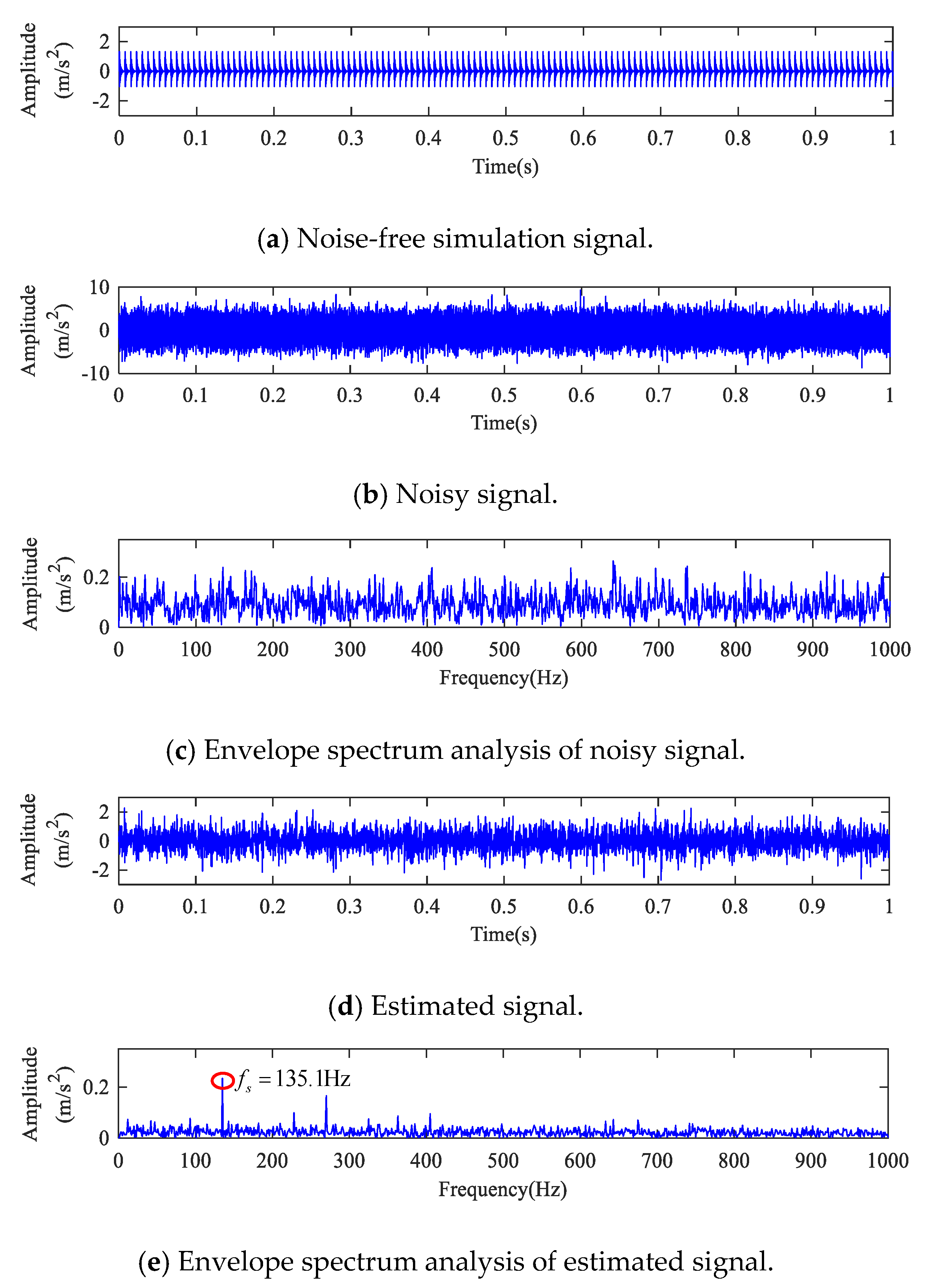
3. Simulation Analysis
4. Experimental Results
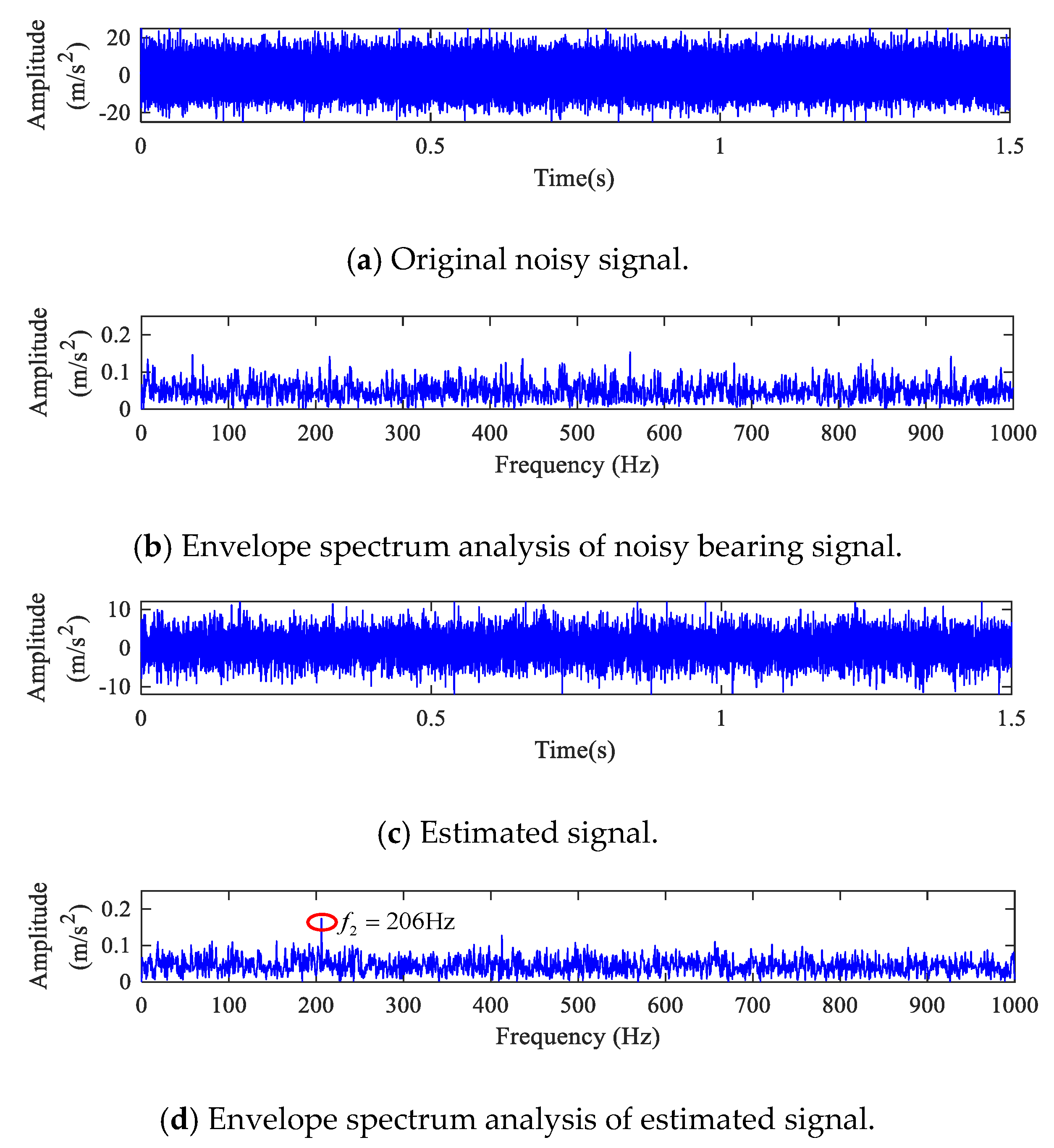
4.1. Outer Race
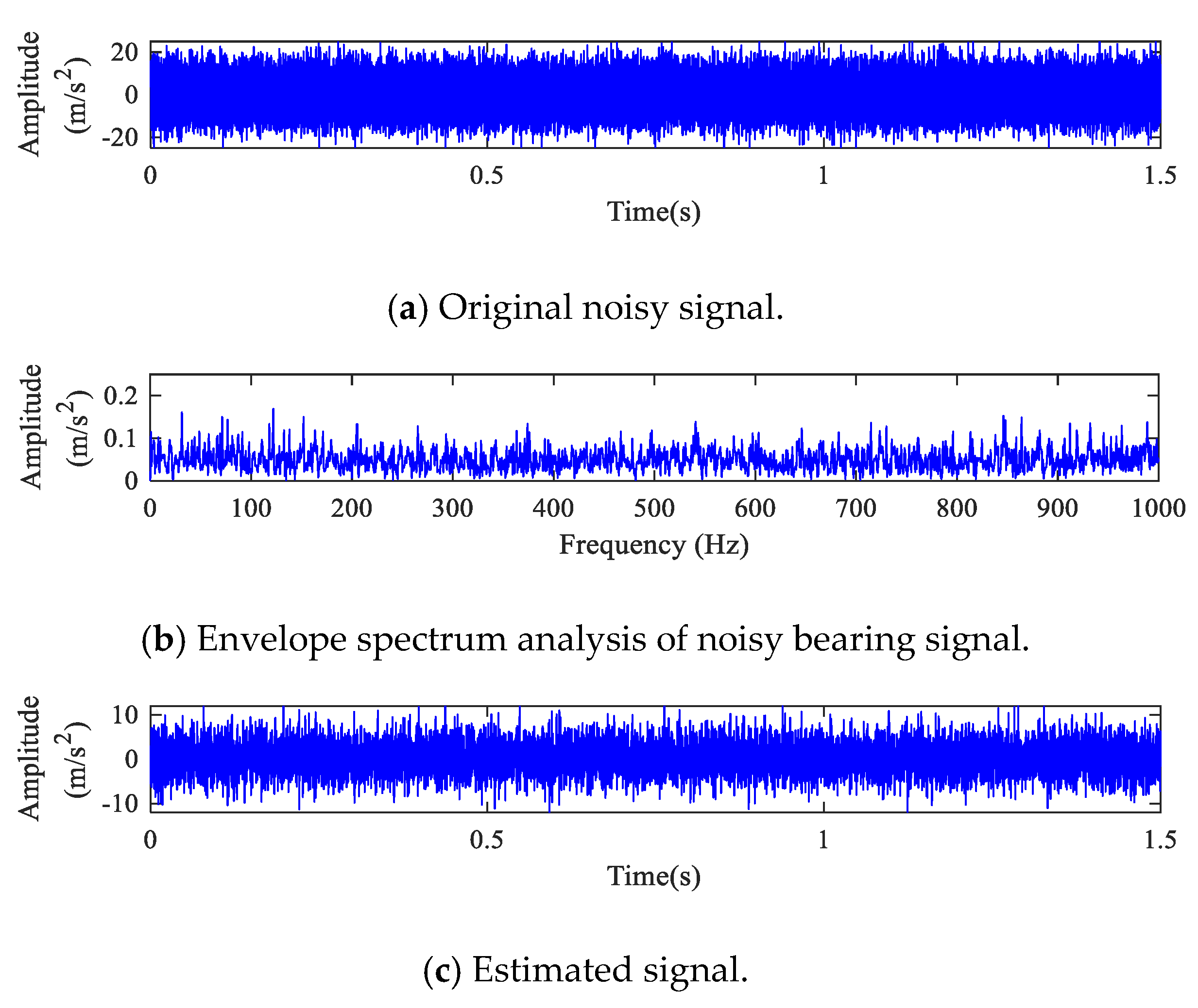
4.2. Inner Race
4.3. Ball
4.4. Computational Complexity Comparison
5. Discussion
6. Conclusions
Author Contributions
Funding
Conflicts of Interest
References
- Wang, J.; Peng, Y.; Qiao, W. Current-Aided Order Tracking of Vibration Signals for Bearing Fault Diagnosis of Direct-Drive Wind Turbines. IEEE Trans. Ind. Electron. 2016, 63, 6336–6346. [Google Scholar] [CrossRef]
- Qin, Y. A New Family of Model-Based Impulsive Wavelets and Their Sparse Representation for Rolling Bearing Fault Diagnosis. IEEE Trans. Ind. Electron. 2018, 65, 2716–2726. [Google Scholar] [CrossRef]
- Liu, Y.; He, B.; Liu, F.; Lu, S.; Zhao, Y. Feature Fusion Using Kernel Joint Approximate Diagonalization of Eigen-Matrices for Rolling Bearing Fault Identification. J. Sound Vib. 2016, 385, 389–401. [Google Scholar] [CrossRef]
- Wang, S.; Chen, X.; Cai, G.; Chen, B.; Li, X.; He, Z. Matching Demodulation Transform and Synchrosqueezing in Time-Frequency Analysis. IEEE Trans. Signal Process. 2014, 62, 69–84. [Google Scholar] [CrossRef]
- Tian, J.; Morillo, C.; Azarian, M.H.; Pecht, M. Motor Bearing Fault Detection Using Spectral Kurtosis-Based Feature Extraction Coupled with K-Nearest Neighbor Distance Analysis. IEEE Trans. Ind. Electron. 2016, 63, 1793–1803. [Google Scholar] [CrossRef]
- Komaty, A.; Boudraa, A.-O.; Augier, B.; Dare-Emzivat, D. Emd-Based Filtering Using Similarity Measure between Probability Density Functions of Imfs. IEEE Trans. Instrum. Meas. 2014, 63, 27–34. [Google Scholar] [CrossRef]
- Yan, R.; Gao, R.X.; Chen, X. Wavelets for Fault Diagnosis of Rotary Machines: A Review with Applications. Signal Process. 2014, 96, 1–15. [Google Scholar] [CrossRef]
- Lu, S.; He, Q.; Kong, F. Stochastic Resonance with Woods-Saxon Potential for Rolling Element Bearing Fault Diagnosis. Mech. Syst. Signal Process. 2014, 45, 488–503. [Google Scholar] [CrossRef]
- Zhao, M.; Kang, M.; Tang, B.; Pecht, M. Deep Residual Networks with Dynamically Weighted Wavelet Coefficients for Fault Diagnosis of Planetary Gearboxes. IEEE Trans. Ind. Electron. 2018, 65, 4290–4300. [Google Scholar] [CrossRef]
- Zhang, H.; Chen, X.; Du, Z.; Yan, R. Kurtosis Based Weighted Sparse Model with Convex Optimization Technique for Bearing Fault Diagnosis. Mech. Syst. Signal Process. 2016, 80, 349–376. [Google Scholar] [CrossRef]
- Gu, F.; Shao, Y.; Hu, N.; Naid, A.; Ball, A.D. Electrical motor current signal analysis using a modified bispectrum for fault diagnosis of downstream mechanical equipment. Mech. Syst. Signal Process. 2011, 25, 360–372. [Google Scholar] [CrossRef]
- Wang, L.; Liu, Z.; Miao, Q.; Zhang, X. Time-Frequency Analysis Based on Ensemble Local Mean Decomposition and Fast Kurtogram for Rotating Machinery Fault Diagnosis. Mech. Syst. Signal Process. 2018, 103, 60–75. [Google Scholar] [CrossRef]
- Chen, D.; Lin, J.; Li, Y. Modified Complementary Ensemble Empirical Mode Decomposition and Intrinsic Mode Functions Evaluation Index for High-Speed Train Gearbox Fault Diagnosis. J. Sound Vib. 2018, 424, 192–207. [Google Scholar] [CrossRef]
- Liu, H.; Huang, W.; Wang, S.; Zhu, Z. Adaptive Spectral Kurtosis Filtering Based on Morlet Wavelet and Its Application for Signal Transients Detection. Signal Process. 2014, 96, 118–124. [Google Scholar] [CrossRef]
- Zhang, Z.; Li, S.; Wang, J.; Xin, Y.; An, Z. General Normalized Sparse Filtering: A Novel Unsupervised Learning Method for Rotating Machinery Fault Diagnosis. Mech. Syst. Signal Process. 2019, 124, 596–612. [Google Scholar] [CrossRef]
- Elad, M.; Matalon, B.; Zibulevsky, M. Coordinate and Subspace Optimization Methods for Linear Least Squares with Non-Quadratic Regularization. Appl. Comput. Harmon. Anal. 2007, 23, 346–367. [Google Scholar] [CrossRef]
- Sun, C.; Wang, P.; Yan, R.; Gao, R.X.; Chen, X. Machine Health Monitoring Based on Locally Linear Embedding with Kernel Sparse Representation for Neighborhood Optimization. Mech. Syst. Signal Process. 2019, 114, 25–34. [Google Scholar] [CrossRef]
- Cui, L.; Wang, J.; Lee, S. Matching Pursuit of an Adaptive Impulse Dictionary for Bearing Fault Diagnosis. J. Sound Vib. 2014, 333, 2840–2862. [Google Scholar] [CrossRef]
- Tian, X.; Gu, J.X.; Rehab, I.; Abdalla, G.M.; Gu, F.; Ball, A.D. A robust detector for rolling element bearing condition monitoring based on the modulation signal bispectrum and its performance evaluation against the Kurtogram. Mech. Syst. Signal Process. 2018, 100, 167–187. [Google Scholar] [CrossRef]
- Bahadorinejad, A.; Imani, M.; Braga-Neto, U. Adaptive Particle Filtering for Fault Detection in Partially-Observed Boolean Dynamical Systems. IEEE/ACM Trans. Comput. Biol. 2018. [Google Scholar] [CrossRef]
- Johansen, A.M.; Doucet, A.; Davy, M. Particle methods for maximum likelihood estimation in latent variable models. Stat. Comput. 2008, 18, 47–57. [Google Scholar] [CrossRef]
- Imani, M.; Ghoreishi, S.F.; Allaire, D.; Braga-Neto, U.M. MFBO-SSM: Multi-fidelity Bayesian optimization for fast inference in state-space models. In Proceedings of the AAAI Conference on Artificial Intelligence, Honolulu, HI, USA, 27 January–1 February 2019; pp. 7858–7865. [Google Scholar]
- Zou, X.; Jancovic, P.; Liu, J.; Kokuer, M. Speech Signal Enhancement Based on Map Algorithm in the Ica Space. IEEE Trans. Signal Process. 2008, 56, 1812–1820. [Google Scholar] [CrossRef]
- Elad, M.; Milanfar, P.; Rubinstein, R. Analysis versus synthesis in signal priors. Inverse Probl. 2007, 23, 947–968. [Google Scholar] [CrossRef]
- Imani, M.; Ghoreishi, S.F.; Braga-Neto, U.M. Bayesian control of large MDPs with unknown dynamics in data-poor environments. In Proceedings of the Advances in Neural Information Processing Systems, Montreal, QC, Canada, 2–8 December 2018; pp. 8146–8156. [Google Scholar]
- Daubechies, I. The Wavelet Transform, Time-Frequency Localization and Signal Analysis. IEEE Trans. Inf. Theory 1990, 36, 961–1005. [Google Scholar] [CrossRef]
- Wang, L.; Cai, G.; Wang, J.; Jiang, X.; Zhu, Z. Dual-Enhanced Sparse Decomposition for Wind Turbine Gearbox Fault Diagnosis. IEEE Trans. Instrum. Meas. 2019, 68, 450–461. [Google Scholar] [CrossRef]
- Wang, L.; Cai, G.; You, W.; Huang, W.; Zhu, Z. Transients Extraction Based on Averaged Random Orthogonal Matching Pursuit Algorithm for Machinery Fault Diagnosis. IEEE Trans. Instrum. Meas. 2017, 66, 3237–3248. [Google Scholar] [CrossRef]
- Donoho, D.L.; Johnstone, I.M. Ideal Spatial Adaptation by Wavelet Shrinkage. Biometrika 1994, 81, 425–455. [Google Scholar] [CrossRef]
- Hansen, M.; Yu, B. Wavelet Thresholding Via Mdl for Natural Images. IEEE Trans. Inf. Theory 2000, 46, 1778–1788. [Google Scholar] [CrossRef][Green Version]
- Jiang, B.; Xiang, J.; Wang, Y. Rolling Bearing Fault Diagnosis Approach Using Probabilistic Principal Component Analysis Denoising and Cyclic Bispectrum. J. Vib. Control 2016, 22, 2420–2433. [Google Scholar] [CrossRef]
- Rabbani, H.; Nezafat, R.; Gazor, S. Wavelet-Domain Medical Image Denoising Using Bivariate Laplacian Mixture Model. IEEE Trans. Biomed. Eng. 2009, 56, 2826–2837. [Google Scholar] [CrossRef]
- Yi, C.; Lv, Y.; Dang, Z. A Fault Diagnosis Scheme for Rolling Bearing Based on Particle Swarm Optimization in Variational Mode Decomposition. Shock Vib. 2016. [Google Scholar] [CrossRef]
- Ding, Y.; He, W.; Chen, B.; Zi, Y.; Selesnick, I.W. Detection of Faults in Rotating Machinery Using Periodic Time-Frequency Sparsity. J. Sound Vib. 2016, 382, 357–378. [Google Scholar] [CrossRef]
- He, W.; Ding, Y.; Zi, Y.; Selesnick, I.W. Sparsity-Based Algorithm for Detecting Faults in Rotating Machines. Mech. Syst. Signal Process. 2016, 72–73, 46–64. [Google Scholar] [CrossRef]
- Cai, G.; Selesnick, I.W.; Wang, S.; Dai, W.; Zhu, Z. Sparsity-Enhanced Signal Decomposition Via Generalized Minimax-Concave Penalty for Gearbox Fault Diagnosis. J. Sound Vib. 2018, 432, 213–234. [Google Scholar] [CrossRef]


| Methods | Spectral Kurtosis | Empirical Mode Decomposition | Time-Frequency Analysis | Sparse Representation | The Proposed Method |
|---|---|---|---|---|---|
| Computational complexity |
© 2019 by the authors. Licensee MDPI, Basel, Switzerland. This article is an open access article distributed under the terms and conditions of the Creative Commons Attribution (CC BY) license (http://creativecommons.org/licenses/by/4.0/).
Share and Cite
Li, S.; Huang, W.; Shi, J.; Jiang, X.; Zhu, Z. A Fast Signal Estimation Method Based on Probability Density Functions for Fault Feature Extraction of Rolling Bearings. Appl. Sci. 2019, 9, 3768. https://doi.org/10.3390/app9183768
Li S, Huang W, Shi J, Jiang X, Zhu Z. A Fast Signal Estimation Method Based on Probability Density Functions for Fault Feature Extraction of Rolling Bearings. Applied Sciences. 2019; 9(18):3768. https://doi.org/10.3390/app9183768
Chicago/Turabian StyleLi, Shijun, Weiguo Huang, Juanjuan Shi, Xingxing Jiang, and Zhongkui Zhu. 2019. "A Fast Signal Estimation Method Based on Probability Density Functions for Fault Feature Extraction of Rolling Bearings" Applied Sciences 9, no. 18: 3768. https://doi.org/10.3390/app9183768
APA StyleLi, S., Huang, W., Shi, J., Jiang, X., & Zhu, Z. (2019). A Fast Signal Estimation Method Based on Probability Density Functions for Fault Feature Extraction of Rolling Bearings. Applied Sciences, 9(18), 3768. https://doi.org/10.3390/app9183768