Article

Failure-Robot Path Complementation for Robot Swarm Mission Planning

1
Department of Automation Engineering, National Formosa University, Yunlin 632, Taiwan
2
Department of Aeronautical Engineering, National Formosa University, Yunlin 632, Taiwan
*
Author to whom correspondence should be addressed.
Appl. Sci. 2019, 9(18), 3756; https://doi.org/10.3390/app9183756
Submission received: 26 May 2019 / Revised: 4 September 2019 / Accepted: 5 September 2019 / Published: 8 September 2019
(This article belongs to the Special Issue Intelligent System Innovation)

Abstract

:
Currently, unmanned vehicles are widely used in different fields of exploration. Due to limited capacities, such as limited power supply, it is almost impossible for one unmanned vehicle to visit multiple wide areas. Multiple unmanned vehicles with well-planned routes are required to minimize an unnecessary consumption of time, distance, and energy waste. The aim of the present study was to develop a multiple-vehicle system that can automatically compile a set of optimum vehicle paths, complement failed assignments, and avoid passing through no-travel zones. A heuristic algorithm was used to obtain an approximate solution within a reasonable timeline. The A* Search algorithm was adopted to determine an alternative path that does not cross the no-travel zone when the distance array was set, and an improved two-phased Tabu search was applied to converge any initial solutions into a feasible solution. A diversification strategy helped identify a global optimal solution rather than a regional one. The final experiments successfully demonstrated a group of three robot cars that were simultaneously dispatched to each of their planned routes; when any car failed during the test, its path was immediately reprogrammed by the monitoring station and passed to the other cars to continue the task until each target point had been visited.

1. Introduction

1.1. Background and Objectives

Currently, unmanned vehicles are applied in various fields. For example, unmanned aerial vehicles (UAV) monitor earth, provide emergency aid, perform disaster control and prevention, and execute aerial photography [1,2]. Along with the mission scale, mission areas are growing much wider and may soon be beyond a single vehicle’s reach. Compared to a traditional single robot system, multi-robots cooperating to achieve a global mission can be used to solve problems for a wide variety of application domains. For example, a multi-robot team is usually beneficial for shortening the time required for a search and rescue mission as well as for reducing energy consumption in large area cargo delivery, etc. All team members cooperate to fulfill a mission by dividing the labor of execution. Controlling unmanned vehicle swarms via human supervision is of great interest in military sectors as well as private logistic companies. While the scope and area of robot vehicle missions is expanding, to complete tasks efficiently (in time or in energy), a well-planned path program for an unmanned vehicle swarm is crucial.
The aim of this research was to develop a group of robot cars as a multi-agent system (MAS) with multi-path programming under the constraint of a maximum distance limit, which is the maximum capable range (usually limited by the onboard battery/fuel energy capacity) of a robot car. With a series announcement of unmanned vehicles’ prohibited zones by government sectors, in addition to optimal multiple-path programming, the system should feature a no-travel zone avoidance function. The no-travel zones serve as a e-fences, which enclose the areas unmanned vehicles are not permitted to enter. The system will process all the target points and then dispatch the optimal paths, which causes the robot cars to avoid the no-travel zone and to reach targets efficiently without wasting precious energy on redundant paths. In addition, for a robot swarm mission, it is recognized that failures (among robot agents) may have a higher chance to occur due to some external/internal factors, such as external attacks or internal mechanical failures, which might affect the success of this endeavor. Thus, there is also an increasing need to develop an algorithm to automatically perform a failure robot’s mission complementation.

1.2. Related Works

Many scholars have conducted studies on path programming, and the path from the start point to the end point is often an essential element. In addition, if there is an obstacle or a no-travel zone on the path, the path programming should consider how to avoid it. In reference [3], Pu-Sheng Tsai et al. applied image processing to detect the obstacle and the turning point, and the Dijkstra algorithm was used to identify the shortest path while bypassing the obstacle. Unfortunately, apart from computer simulations, there is no field experiment to validate this research. The A* Search algorithm [4], developed in 1968 based on a best-first search and Dijkstra’s algorithm, has proven to have a better performance than Dijkstra alone by combining the advantages of the two algorithms. It has been widely applied to determine the optimal path for online game characters and some industrial carriers from current locations to specified destinations [5,6].
In terms of path programming and scheduling for multiple target points and multiple vehicles, for years, many studies have focused on solving the vehicle routing problem (VRP) and the multiple traveling salesman problem (MTSP). As Figure 1 shows, MTSP involves m salesmen who must visit a set of n cities; each salesman starts and ends at the same place (city), and each city must be visited exactly once by one salesman. The objective of the problem is to find the shortest total distances travelled by all the salesmen. In practice, each salesman has similar abilities and limitations; therefore, using MTSP with an ability constraint is more appropriate for studying real-world problems. For example, it is unrealistic that one salesman would travel to all the cities, while others would visit only one city. As such, the number of cities to which each salesman travels is limited [7]. The multiple traveling robot problem (MTRP) further extends the traditional traveling salesman problem (TSP) and involves a team of robots visiting target points at least once (and ideally more than once). The overall solution quality is dependent on both the quality of the solution constructed by the paths of the robots and the efficient allocation of the targets to the robots [8].
In this NP-hard problem, the complexity of the solution increases as the number of target points increases. Because it is almost impossible to go through all the feasible paths and to determine the best solution within an acceptable timeframe, heuristic algorithms have been adopted to obtain approximate solutions. Majid Yousefikhoshbakht et al. [9] used a new modified ant colony optimization (NMACO) mixed with insert, swap, and 2-Opt algorithms as well as an efficient candidate list to improve the efficiency of ant colony optimization (ACO). Yousefikhoshbakht’s algorithm is quite competitive with other meta-heuristic algorithms, which have solved a library of sample instances for the traveling salesman problem (TSPLIB); however, the solution it yielded can still be improved. Raluca Necula et al. [10] used five modified ACOs to solve MTSP. The maximum number L and minimum number of cities that each salesman should visit K were defined and limited to solve MTSP instances using the TSPLIB. Furthermore, Mingji Xu et al. [11] used a hybrid genetic algorithm (GA) and simulated annealing (SA) to solve MTSP, enhancing the local search ability to achieve a better global optimal solution than could be obtained using a general GA; however, the solution was proven not to be the best in later research. Using ACO and GA to solve MTSP problems may not always yield consistent solutions even under exactly the same initial test setting, and each case must be tested continuously to converge the best solution.
Jean-François Côté et al. [12] used the Tabu search (TS) to solve the VRP and to test it with benchmark instances. The test results not only achieved convergence in a reasonable time but were also superior in distance for the benchmark instances.
Wan-shu Huang and Tsai-Yun Liao [13] used a two-phased method to identify an optimal solution to solve the dynamic vehicle routing problem (DVRP). Unlike MTSP, DVRP limits the vehicle capacity. Fuzzy C-mean techniques were used to divide existing customers, while a cost function was adopted to determine the initial solution in the first phase. In the second phase, TS was combined with 2-opt and or-opt to improve the cross-routes and in-routes, respectively, and to solve the problem related to multi-vehicle path programming.
In their research on MTRP, Sanem Sariel-Talay et al. [8] mentioned that their system could determine real-time optimal paths for traveling among multiple target points on their own platform with a robot swarm; they successfully completed the assignment as well as the failure complementation; however, this trajectory was not the best solution. Because when failure occurred, a failed robot’s unfinished duty could be carried out by other healthy robots only when they had finished their own original assigned paths. In addition, this solution did not consider the maximum distance limit (battery power limit).
There have been numerous studies and scholarly journal articles on multi-vehicle path programming, but on-site experiments with cars to verify the effectiveness of the programming are rare. Moreover, these studies do not include a no-travel zone or vehicle failure conditions. In MTSP, the maximum and minimum numbers of cities that each salesman should visit are defined and limited, but the tasks may still fail to be completed due to the limited energy source mounted on each car. Thus, in the present study, a maximum distance limitation was added.
To focus on the issues of maximum distance and vehicle failure, a mathematical model along with a distance array were set for path programming. If any path programmed covered the no-travel zone, the A* Search algorithm was adopted to find an alternative path. Then, the two-phased module served as the solution module. In the first phase, TS was combined with the 2-opt swap method to program a single optimal path, and an initial solution was obtained by splitting the path into multiple sub-paths. In the second phase, Wan-shu Huang and Tsai-Yun Liao’s solving module, which combined TS with the 2-opt swap method to improve in-route and cross-route solutions, was adopted. The modified module improved the application of TS on cross-route programming and ensured the solution would not exceed the maximum distance. A diversification strategy, which was similar to the GA, was implemented for in-route path improvements. This strategy recorded and selected the optimal solution or the second-best solution as the initial solution for in-route path improvement later so that an unwanted regional optimal solution could be avoided. The second phase was operated repeatedly until the termination conditions were reached.
In the final phase, this solution was verified by experiments using real robot cars running on the programmed paths. If any vehicle in the swarm failed, its unfinished route was randomly inserted into the other route as an initial condition, and then a re-programming process began immediately. After the experiments were completed, the distance of paths generated from the path programming algorithm and the differences between the trajectories of the actual and theoretical paths were examined.

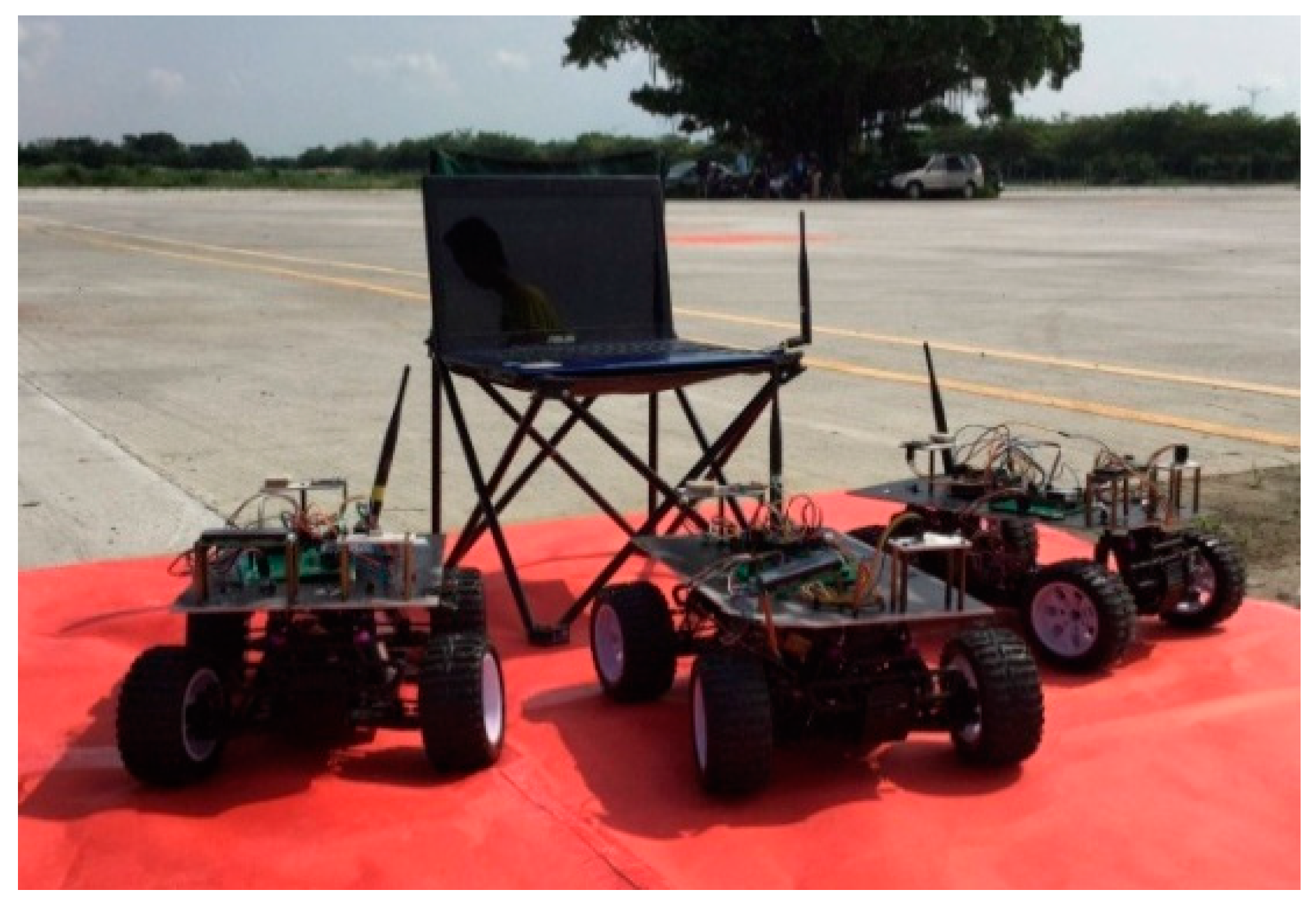
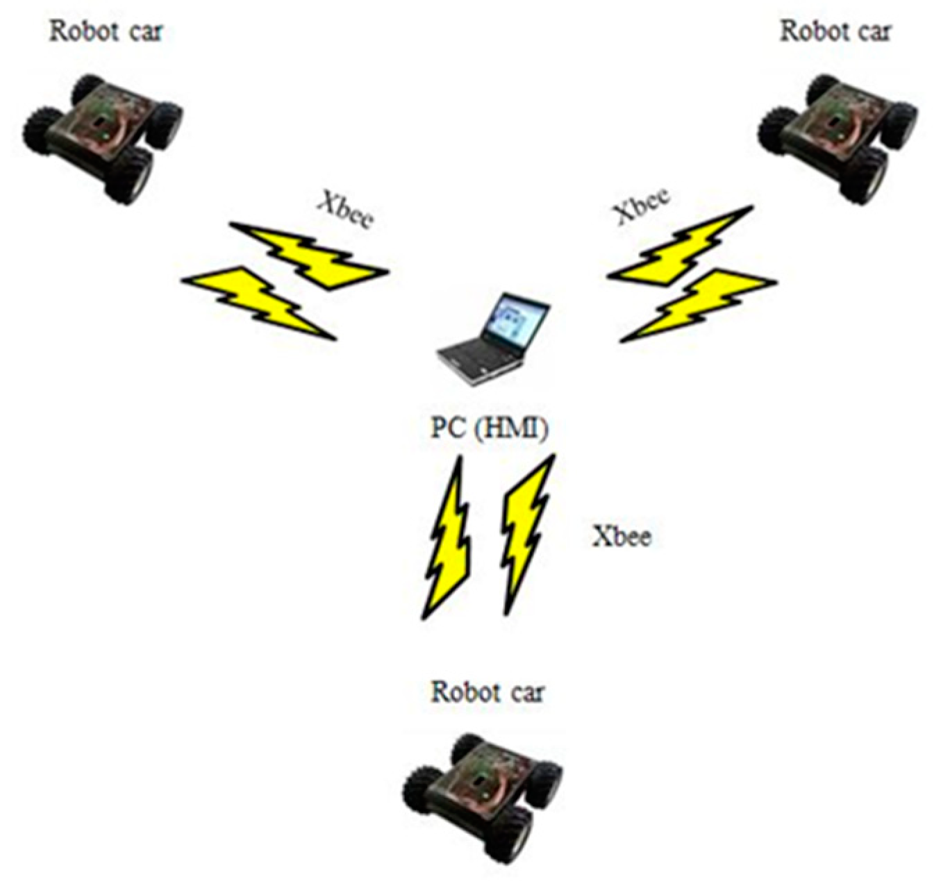
2. Experimental Vehicle and System Architecture

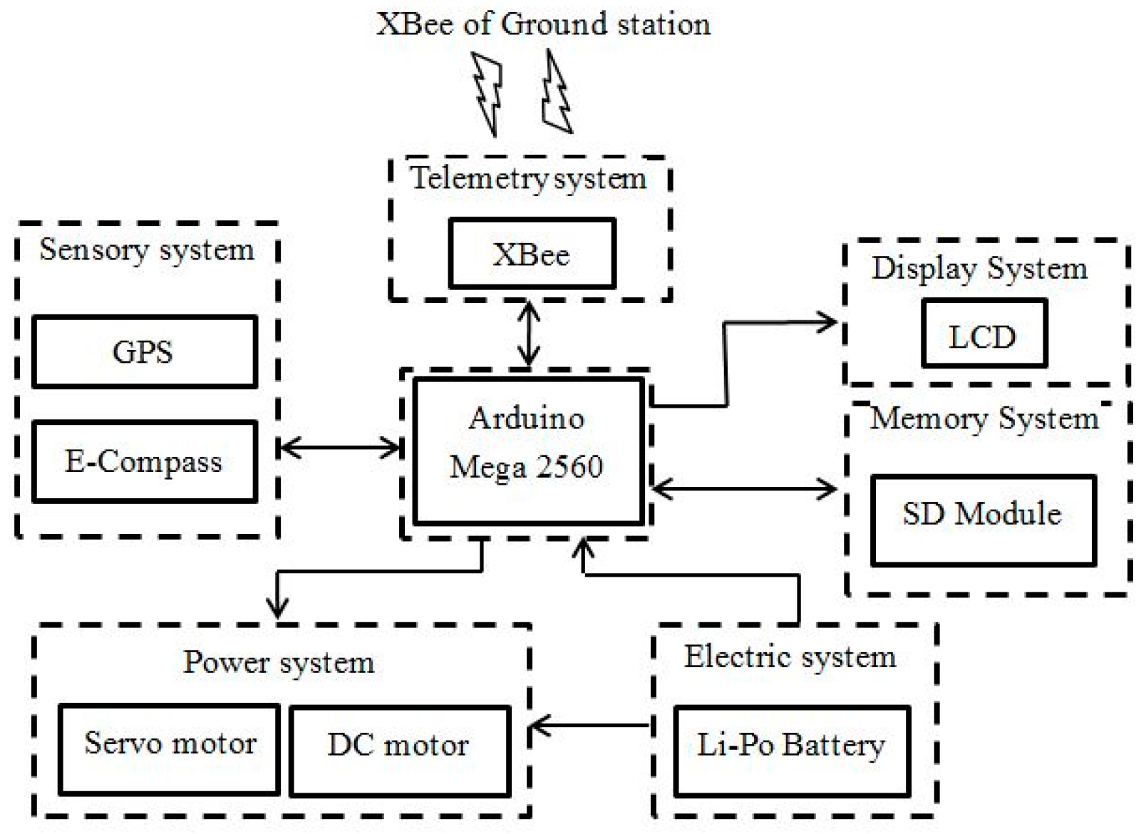
2.1. System Architecture

As the aim was to complete the task with multiple target points using multiple vehicles in the shortest time required, a MAS under a central control was created for this research. The central control allocated assignments to each individual robot and allowed them to complete the tasks independently rather than controlling the cars throughout the experiments. Through cooperation between multiple agents, the system was able to complete larger scale tasks that could not be completed by a single vehicle. From the MAS viewpoint of task allocation, the system consists of single-robot tasks, single-task robots, and the instantaneous allocation of tasks (ST-SR-IA) [14].
Various assignments at different levels of difficulty were randomly allocated by the system; this means that each robot car could receive any assignment regardless of the difficulty. Thus, each car in the robot swarm had to be equipped with identical specifications to ensure its performance and capacity to cope with various assignments. From the viewpoint of MAS heterogeneity, the degree of similarity between individual robots within a collection H e t ( R ) was as follows:
Het ( R ) = i = 1 C a s t e p i log 2 ( p i )
where C a s t e is the type of robot, and p i is the decimal percent of a robot belonging to any caste. All specifications in this system are the same (caste = 1, pi = 1), and Het ( R ) = 0 (Equation (1)) [15]. Thus, this system is a homogeneity system of a robot swarm.
Figure 2 illustrates the full system, which includes a remote monitoring station, a multi-vehicle path programming system, and robot cars, and Figure 3 illustrates the system architecture. The remote monitoring station is a laptop with CI7, 2.4 GHz, and 8 GB RAM. It serves as a central controller that can program and distribute the paths to the robot swarm, which is designed to complete the work together. From the viewpoint of network topology, this system is similar to a star topology. The system mainly uses LabVIEW to develop a portable remote monitoring station interface by sending a URL to obtain the Google Maps web page as a display interface. It can be used as a man–machine interface (MMI), where vehicle location feedback and the initial path programming could be displayed and managed. By clicking on the target points displayed on the MMI, the location is sent to the portable remote monitoring station where the path programming algorithm is running. Then, the planned paths can be passed to each car via XBee. Once the cars receive the data, they can engage the brushless motor to move forward and control the servo motor differential to complete the assignment successfully.

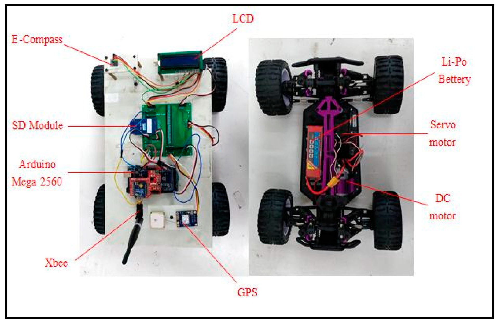
2.2. Experimental Vehicle

Three robot cars were used as the experimental vehicles in this research (see Figure 4 for the architecture diagram). Their function was to receive data on target points from the remote monitoring station and to establish a database for the route. Once a car arrived at its designated target points, the real-time locations were provided immediately to the remote monitoring station.
The experimental vehicles were modified from remote control trucks. The car shell and the infrared remote control equipment were removed, and a piece of white ABS board was mounted to carry commercial off-the-shelf electronic parts for the autopilot function. The component configuration is shown in Figure 5.

3. Design and Principle of Path Programming

The problem definition in this research was modified from a standard module Single-Depot MTSP (SD-MTSP) [16]. The object and subject are as follows:
x i j k = { 1 0 the   k   path   goes   from   city   i   to   city   j otherwise
( i , j ) A , k = 1 , m
Object:
m i n k = 1 m ( i , j ) A c i j x i j k
Subject to:
( i , j ) A c i j x i j k D l m t , k = 1 , m
k = 1 m j = 2 n   x 1 j k = m
k = 1 m j = 2 n   x j 1 k = m
k = 1 m i = 1 n   x i j k = 1 ,   j = 2 , , n
k = 1 m j = 1 n   x i j k = 1 , i = 2 , , n
k = 1 m x i 1 k + x 1 i k 1 , i = 2 , , n
u i 1 ,   i = 2 , , n
where c i j is the distance array of A, m is the number of robot cars, D l m t is the maximum distance limit value, n is the number of target points, and u i is the number of target points to be visited along one car’s path from its original point to a specific target i. (2) is the variable integer, which determines whether targets i to j have been traveled by k car. In (3), A is the set of all specified paths, including the alternatives that do not bypass the no-travel zone, while (4) is the object function of this problem. Per (5), the subject D l m t cannot be exceeded by all the cars, and (6,7) ensure a start from the original point and a return to that same point. Per (8,9), all the targets are entered and exited by the car, and per (10), each car must visit at least one target. Finally, (11) prevents the problem of a sub-path that does not include the original point. This is an NP-Hard problem, and heuristic algorithms are always adopted to solve this type of complicated optimization problem. While there are many types of heuristic algorithms, the A algorithm and the TS heuristic algorithm were primarily adopted.

3.1. A* Search Algorithm

The evaluation function f ( n ) is the core of the A* Search algorithm. As shown in function (12), it is the aggregation of g ( n ) and h ( n ) ; g ( n ) is the travel distance from the start point to any specified node n, and h ( n )   refers to the linear distance from any node n to the target point.
f ( n ) = g ( n ) + h ( n )
The algorithm provides a better evaluation function, which is capable of efficiently determining the optimal path between the start point and the end point; therefore, it was used to program paths bypassing the no-travel zone.

3.2. Tabu Search (TS)

Tabu can imitate human memories, maintaining experiences of the past to prevent roundabout searches and creating a Tabu list. It can learn from past solutions to avoid having a regional optimal solution be viewed as a global optimal solution. As long as the initial solution and the Tabu list for TS are well set, a convergence can quickly be completed and the optimal solution can be obtained, which is highly stable in a solution’s consistency [2]. The Tabu search first establishes an initial solution and then determines the neighborhood optimal solution or accords the solution of aspiration criterion as the basis for moving. This means searching for solutions in the neighborhood domain of the current solution. Among them, the Tabu list memory mechanism is notably important; it records the solutions that have already been searched to prevent useless or redundant searches. Once the search of the entire neighborhood domain is completed, the optimal direction in which the cars should move is selected. If any solution is found that is better than the optimal solution, then the optimal solution is updated; this process proceeds until the termination condition is reached [17]. TS combined with the 2-opt nodal line swap method, proposed by Lin in 1965 [18], was adopted in the present study to change the order of the path to expand the current solution. Initially, it was designed for TSP, but now it is widely used in solving various path problems, including TSP, VRP, and VRPTW (Vehicle Routing Problems with Time Windows).

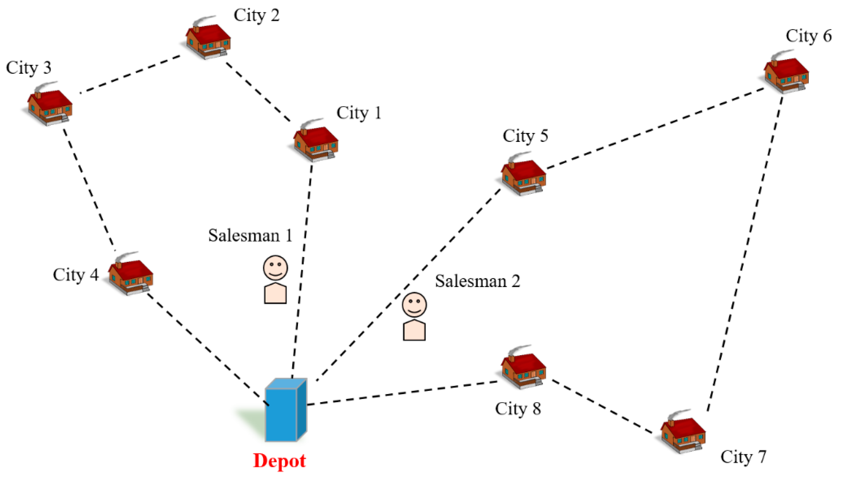
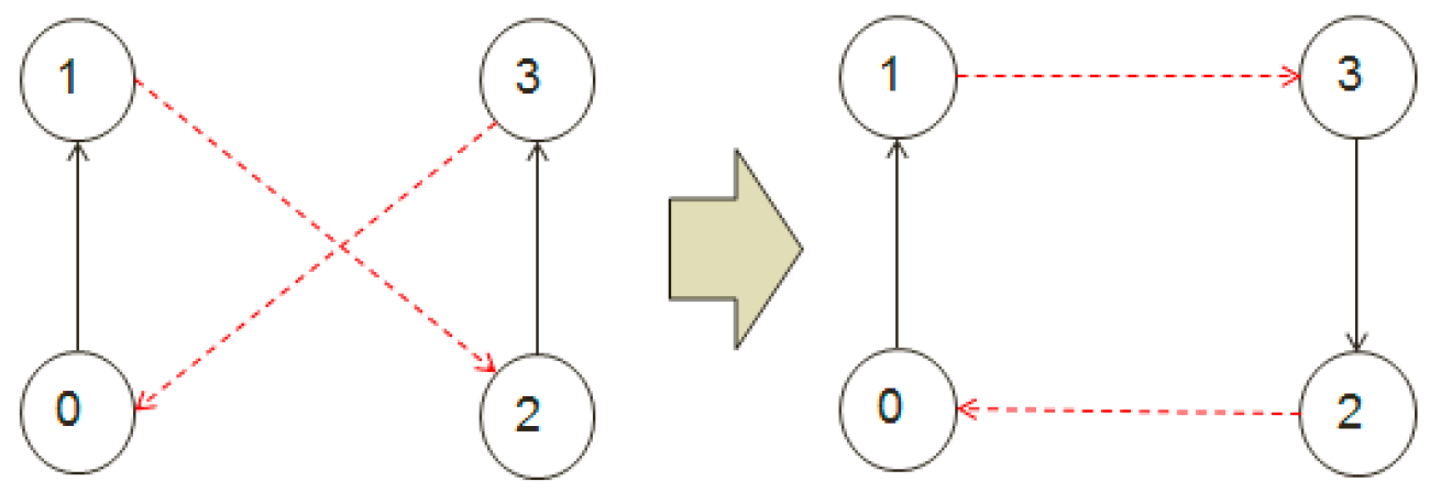
3.2.1. TS to Program the Single Path (In-Route)

TS combined with 2-opt was adopted to improve the in-route path programming for a single path. The 2-opt in-route swap concept is shown in Figure 6. If the (1,2) and (3,0) nodal lines are replaced, then (1, 3) and (2, 0) can be connected to change the path.
Therefore, 2-opt was used as a movement method to solve the single optimal path problem. Also, the length of the Tabu list, the stopping criteria, and the initial solution were set at this time. Then, the executed TS was used to determine the optimal single path.

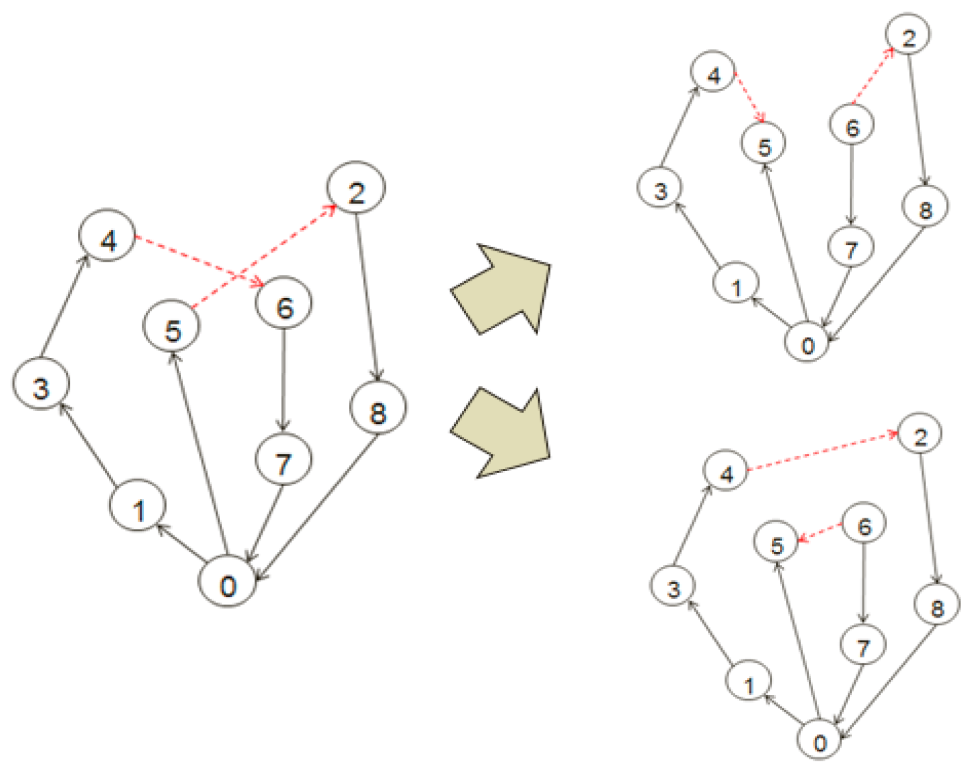
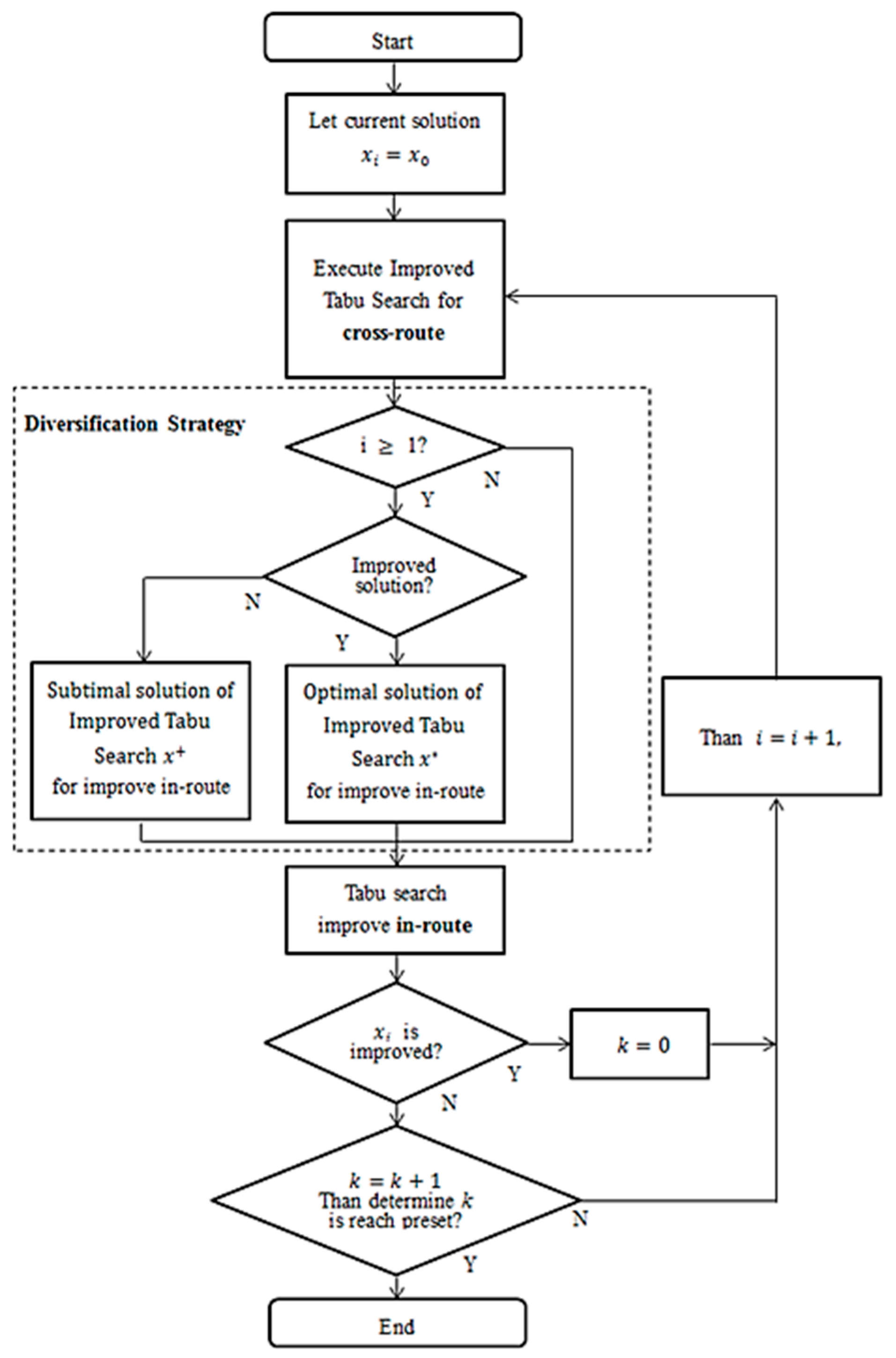
3.2.2. Improving TS to Improve the Cross-Route Path

The algorithm of improved TS combined with 2-opt was used to improve the cross-route path in this research. By moving based on 2-opt, the nodal lines were swapped between different paths to improve the current paths. As shown in Figure 7, the method for a cross-route path swap was different from the one used for the single path. Exchanging the unfavorable (route crossed) swap nodal lines of (4,6) and (5,2) creates two different possible paths: (4,5) and (6,2) as well as (4,2) and (6,5). Compared to the former, the latter also changes its direction. Thus, 2-opt can reverse the direction of the paths.
The key point of the improved TS is to set the S l m t variable, which contains solutions exceeding the maximum distance limitation, and the solution exceeding S l m t is removed from the candidate list to ensure that all path solution values are within range. This limitation may result in an empty set for the candidate list, blocking all solutions from entering the next generation; therefore, an original Tabu list was adopted with S l m t , the solution set containing all solutions, even those exceeding the maximum distance limitation. With the loosened criteria, the search also selected the “distance of the longest traveling path” as the solution of the minimum value.
Therefore, 2-opt was applied to improve cross-route paths, and the length of the Tabu list, the stopping criteria, and the initial solution were set at this time. Then, the improved TS was executed to determine the optimal multi-paths.

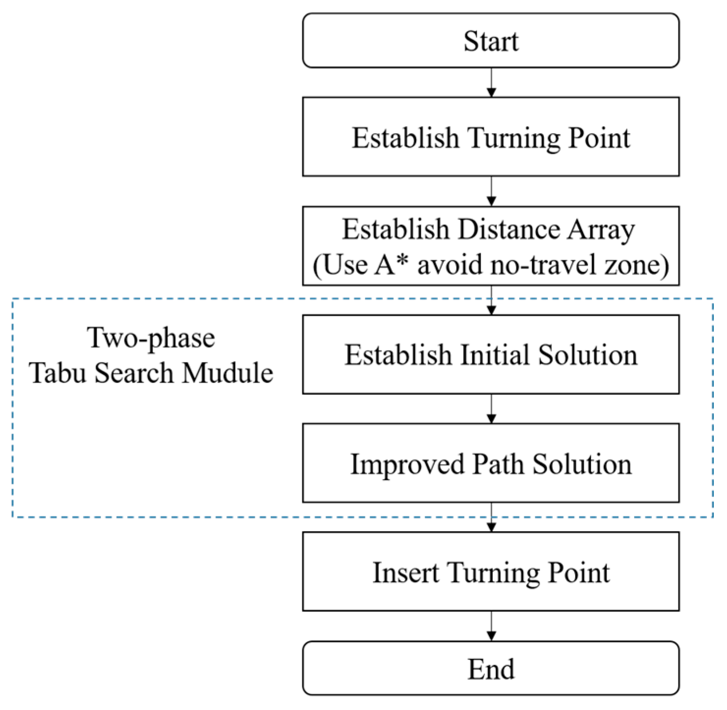
3.3. Workflow of Multi-Vehicle Path Programming

In this research, TS was selected as the core algorithm, and the A* Search was adopted as a supplement for path programming. The flow chart is shown in Figure 8.

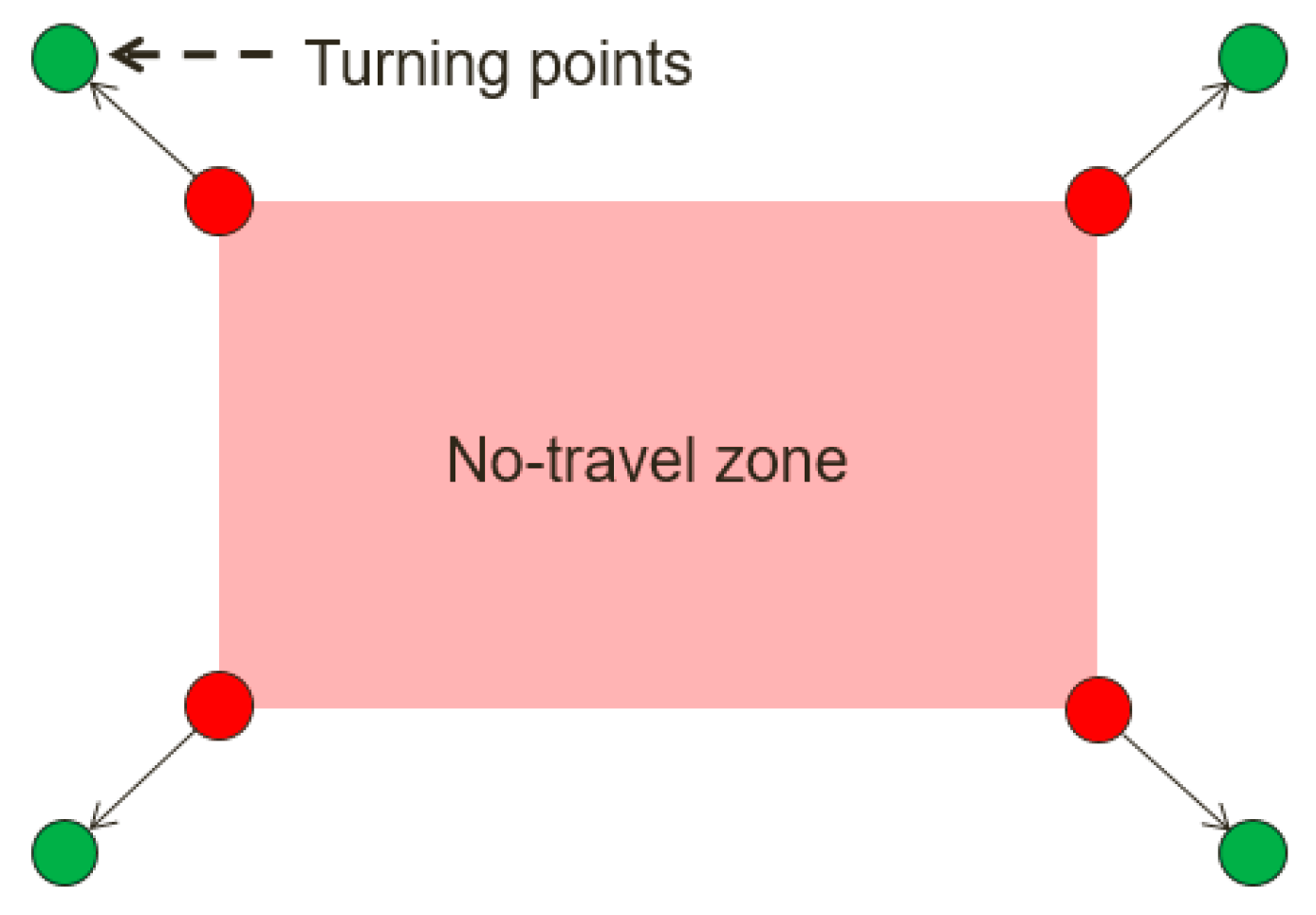
3.3.1. Establishing the Turning Points

The schematic diagram of the turning points is shown in Figure 9. To ensure that all paths between nodes did not pass through the no-travel zone, the turning points were automatically generated at meters away from the outer corners similar to a bubble covering a no-travel zone when a prohibited zone appeared on the working area of the e-map. When the algorithm is run using a computer, if any route touches the bubble, these turning points on the corners were treated as new “nodes” and then incorporated into the re-routing process. Hence, robots were guided away by the new nodes. The formula for calculating the turning points is as follows:
P c = 1 m no i = 1 m no P i
P new = P c + a ( P i P c )
The center point P c from (13) was inputted into (14) to determine the turning points, a is the ratio of enlarging the area, P c is the center point, Pi are the corner points of the no-travel zone, m no is the number of corner points, and P new is the turning point after enlarging the area.

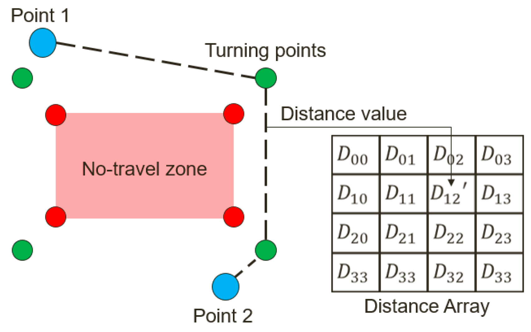
3.3.2. Establishing the Distance Array (Using A* to Avoid the No-Travel Zone)

All data on the distance between nodes has been stored as a distance array, and distance information can be accessed from the array without spending time on redundant calculations.
As shown in Figure 10, there is a no-travel zone on the map. Before programming the route of the system, the A* search was applied to determine whether there were any linear paths between any two points touching the zone (such as blue points 1 and 2). If there were, the A* search was used to determine alternative paths using turning points to bypass the no-travel zone. Once the turning point was used, the distance information of the new curved-route was provided to update the distance array. If there were not, the original algorithm continued running until all distances between targets were known.

3.3.3. Establishing the Initial Solution

The formation of the initial solution was processed through three steps. In step 1, the nearest distance method was used to generate a rough plan for single path programming. First, the distance array c i j was established, and the zeroth row of c i j = . Then, the point in which the row of c i j had the minimum value was set as the 1st point, and the value of this row of c i j was set at infinity. Then, the same procedure was repeated to search and to set the 2nd point, the 3rd point, etc. The initial solution was repeated until all the points were searched. In step 2, TS and 2-opt were used to optimize the single path. In step 3, the single path was divided into multiple sub-paths, which were as short as possible, and the maximum distance limit was set; these multiple sub-paths formed the initial solution for the next phase.

3.3.4. Improved Path Solution

This section covers general path programming, and path complementation for failed tasks is discussed in the next section. As the path could be improved and converged into the optimal solution, this critical method was applied as the core of this study.
In this phase, the 2-opt rules were followed to swap the node lines in the in-route and cross-route movement paths, and the solution gradually converged into the optimal solution. At this point, the distance summation of all paths was minimized to ensure that the assigned distance of each robot car did not exceed the maximum distance limit. The flow chart is shown in Figure 11. First, the flow of the improved TS was executed to improve the cross-route. Then, the single path of each group that was not improved by TS was improved. Until each group was improved, the flow returned to the step involving the improved TS for cross-route path programing.
When this phase proceeded to the second generation, part of the cross-route improvements could identify a solution that had not been improved and that could be identical to the one obtained in the first generation. If this solution was used to calculate the in-route, it could result in a useless local optimal solution without any further improvements. To avoid this situation, it should be determined whether this solution was improved before proceeding to the second generation. If not, the suboptimal solution from the cross-route path exchange should be implemented for improvement to end the local optimal solution loop and to obtain the global optimal solution.

3.3.5. Inserting the Turning Point

If no turning point in the optimal path solution is generated, the turning points generated from the A* search should be inserted into the path that passes through the no-travel zone.

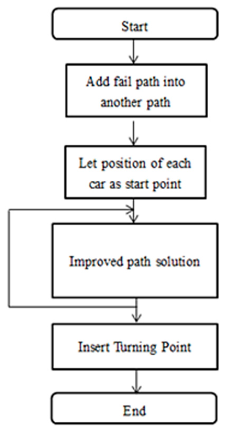
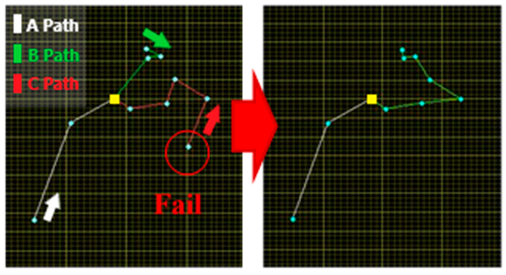
4. Complementation for the Failed Path

When any vehicle fails on the way to complete its task, it is critical to activate the path re-programming and to re-allocate paths and new target points to the rest of the robot cars with the most efficient solution to eventually complement the incomplete tasks.
This is slightly different from the regular path programing process mentioned. Programming for a failed path has a different start point but the same end point and must ensure that the remaining target points are visited one-by-one. A model with m robot cars and one car that failed to complete the task is described as follows:
x i j k = { 1     0     the   k   path   goes   from   city   i   to   city   j otherwise
( i , j ) F
Object:
m i n k = 1 m ( i , j ) F c i j x i j k   + k = 1 m 1 i = n + 1 n + m 1 j = 1 n c i j x i j k
Subject to:
( i , j ) F c i j x i j k + k = 1 m 1 i = n + 1 n + m 1 j = 1 n c i j x i j k   D l m t   , k = 1 , , m 1
j = 1 n   i = 1 m 1   x ( n + i ) j k = 1 ,   k = 1 , , m 1
k = 1 m 1 j = 2 n + m 1   x j 1 k = m 1
k = 1 m 1 i = 1 n + m 1   x i j k = 1 ,   j = 2 ,   , n
k = 1 m 1 j = 1 n   x i j k = 1   ,   i = 2 ,   , n
(15) is a variable integer that determines whether k car runs through the path from target i to target j. In (16), F is the aggregation of all nodal lines between unvisited targets, while (17) is the target function of this question, which aims to determine the shortest path for the active cars to return to the original start point after they visit all targets. (18) to (22) are constraints; (18) mainly constrains the total distance run by all active cars, which must travel to all targets and return to the start point without exceeding the maximum limitation. (19) and (20) constrain the start point to each car’s current location i = n + 1 , , n + m 1 , and each car should end at the original start point i = 1 . (21) and (22) ensure that each target point is entered and exited only once.
To solve the issue of failure complementation, a set of strategies was designed, as shown in Figure 12. First, the failed car’s remaining path was randomly assigned to the other cars, and path improvement was executed using TS combined with the 2-opt swap method. Unlike the original TS, which had the same start and end points in path programming (path solution x = { P 0 , P 1 , , P n , P 0 } ), the path programming for complementing the failed path changed the starting point but maintained the same end point (path solution x = { P n + 1 ( or P n + m 1 ) , P 1 , , P n , P 0 } ; P n + 1 , , P n m + 1 is the latest location of active cars).
Usually, the two types of paths described would be generated, while the 2-opt swap method is adopted to program multiple paths. The path programming for the failed path does not adopt a solution that may cause reversed routes in order to avoid leading the path back to the original start point.
The steps for the solution are as follows:
Step 1: The failed car’s remaining path is randomly inserted into any path, and the number of cars dispatched is set as   m = m 1 .
Step 2: Because the first index from the solution of the remaining path does not refer to the cars’ current locations, the locations of the individual cars P n + 1 , , P n + m 1 are inserted into each path, respectively, as the start points.
Step 3: The path solution, as adjusted by steps 1 and 2, is used as the initial solution x 0 for path improvement. With the in-route and cross-route paths improved, the optimal solution generated would be the best path for complementing the failed path.
Step 4: The turning points are inserted into the path that passes through the no-travel zone.

5. Path Programming and Experiment Results

5.1. Test of Computer Path Programming

The aim of this research was to solve the path programming of a wide multi-target area. Subject to vehicle ability constraints, cars are not able to travel to all target points. A hybrid TS combined with the 2-opt swap method was adopted. To establish the initial solution, the Tabu list length was set to 30 (ITL = 30), and the condition set for stopping was that the optimal solution was not updated and improved in 50 generations (ISC = 50). The Tabu list length of the improvement of each single path was set to 30 (IRTL = 30), and the Tabu list length of the improvement between different paths was 30 (CRTL = 30). The condition set for stopping the calculation for path programming was that the solution was not updated and improved in the most recent 50 generations (IRSC, CRSC = 50). The condition set for stopping the path improvement was that the optimal solution was not updated and improved in the 2nd iteration (TSC = 2).

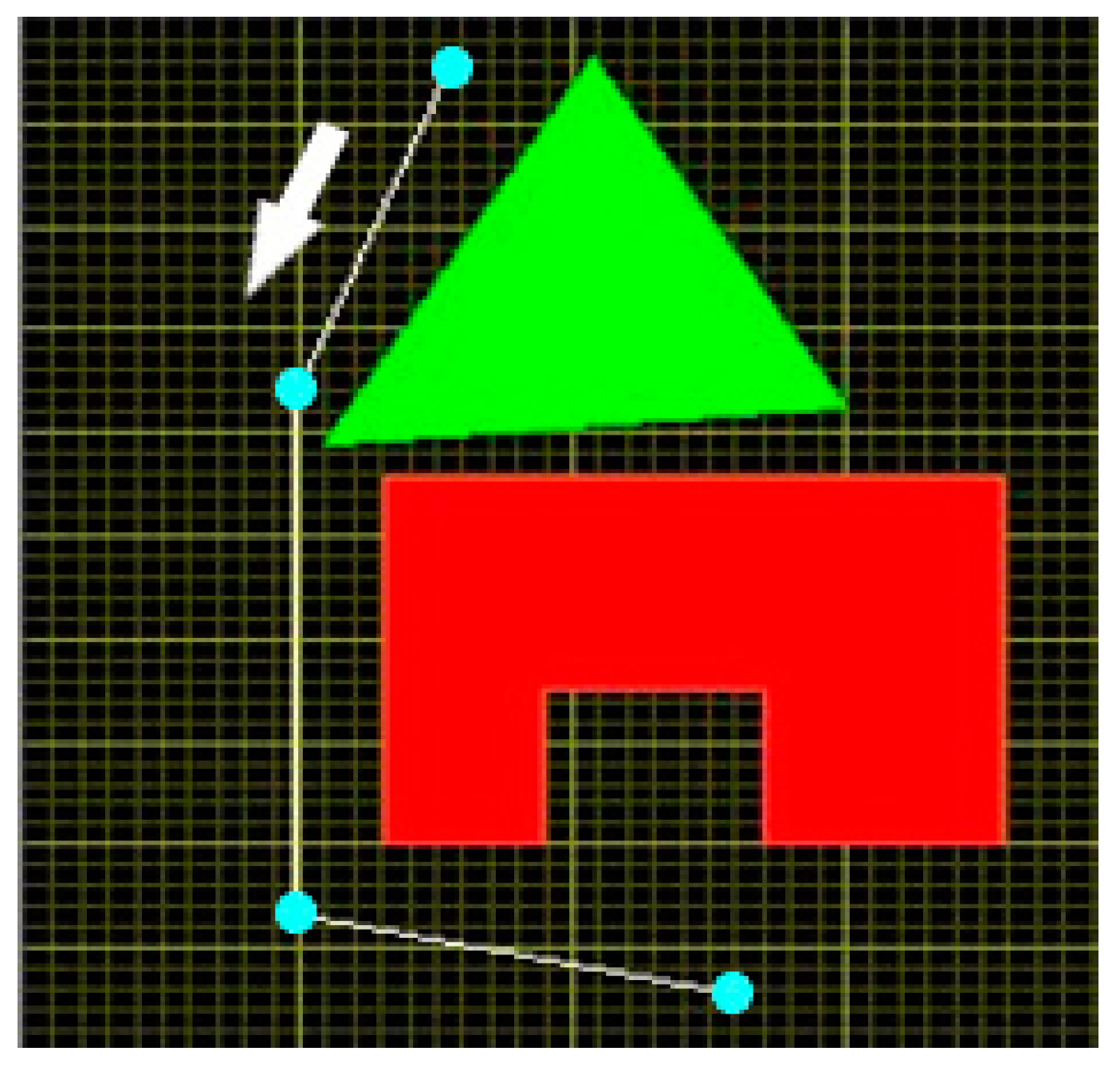
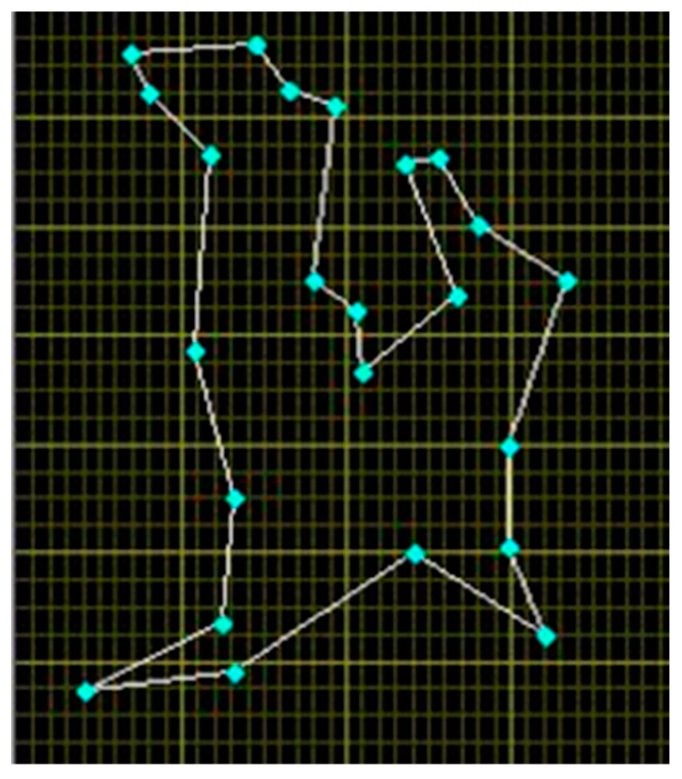
5.1.1. Test of the Path Bypassing the No-travel Zone

To ensure that the path programed by the A* search did not cross the no-travel zone, a double no-travel zone was implemented for this test. Figure 13 illustrates the test result; the car successfully bypassed the enlarged zone within the turning points set.

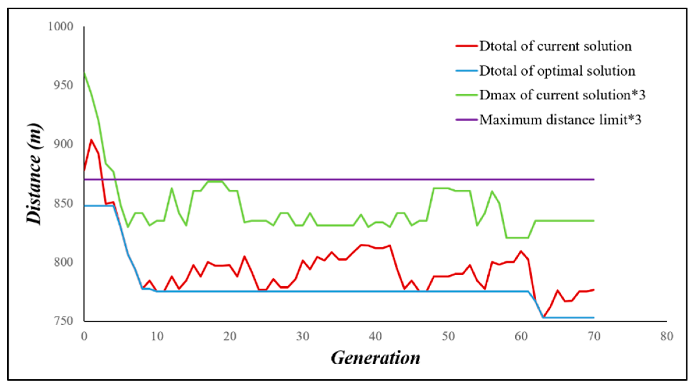
5.1.2. Test of Path Scheduling and Algorithm Convergence

A simple 22-point test was used to ensure algorithm convergence. The maximum distance limitation was set at 290 m. For single path programming, the optimal path generated is shown in Figure 14. With a total distance of 660.5 m, which exceeds the maximum value, it is clearly proven that no single vehicle is capable of completing this task. The optimal path in Figure 15 was generated by the algorithm designed in this research. It illustrates a total distance of 752.8 m and a maximum distance of 278.4 m, neither of which exceed the maximum limitation. As shown in Figure 16, the solution converged at the 63rd generation. The solution was not immediately improved in the first generation. The solution exceeded the maximum distance limit, and the Candidate List = N ( x i ) T S l m t = . Please note that N ( x i ) is the neighborhood solution set of the current solution, T is the Tabu list that collected the past solutions, and S l m t is the set of the maximum distance limits. In other words, the improved TS was followed, and the Candidate List = N(xi) − T was liberalized. The maximum distances of all paths were compared, and the solution with the minimum value in the candidate list was selected. The maximum distance limit is a function that constrains the maximum distance of all feasible solutions and is not allowed to exceed this threshold. Starting from the maximum distance, the minimum maximum distance of the neighborhood solution is selected, and then the current solution gradually becomes closer to the threshold (maximum distance limit) and eventually approaches the threshold. Finally, the current solution is eligible (see the green line in Figure 16, which is the distance variation of the current solution). At the same time, the current solution is improved and gradually moves closer to the feasible solution.

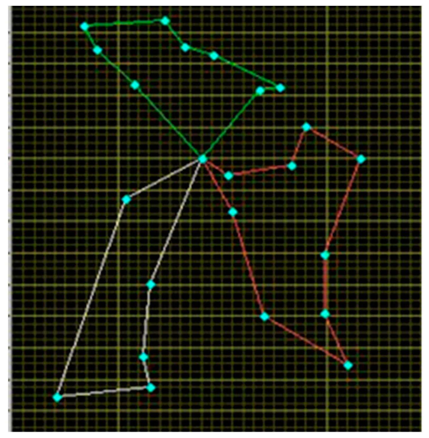
5.1.3. Test of Complementation of the Failed Task

The final test conducted for this study was the test of failure complementation. Failure occurred in the case mentioned in which one car failed to complete the task. As illustrated in Figure 17, the car running on the C path (red) failed. At this point, each robot car had run 135 m and still had 155 m remaining to hit the targets (yellow square); therefore, 155 m was set as the maximum distance limit for failure complementation path programming.
After re-allocating the path, the failed task and path were complemented by other active cars. The total distance was 246.7 m, while the maximum distance was 142.6 m, which was less than 155 m, the distance limit of the remaining path.

5.2. Benchmark Test and Comparison

The problem definition of this study is similar to MTSP except that this research is limited to the travel distance of each robot car. Therefore, the innovative algorithm developed for this research was used to solve the MTSP problem for comparisons. Mingji Xu et al. [11] set 50 target points to test the modified simulated annealing genetic algorithm (MSAGA). For this research, a new algorithm was tested with the same instance as in Xu’s research and was compared to the result of Xu’s algorithm.
Table 1 shows the results of the distance comparison to other three algorithms. The row named 2TS+2OPT is the improved two phase Tabu Search and 2-OPT algorithm which established in this research, n is the number of targets, m is the number of salesmen (or vehicles), and the unit for all distance values are in unit steps.
The algorithm used for this research runs on a system’s monitoring station, which is a laptop PC with Core I7 2.4 GHz CPU and 8 G RAM. Compared to the benchmark tests for HGA, SA, and MSAGA, the distance value for 2TS+2OPT is superior when the number of nodes (n) increases. By the comparison of the simulation results of the four algorithms in Table 1, it is clear that improved 2TS+2OPT is able to converge to a better solution that allows robot vehicle swarm operating in a more efficient way; however, it is difficult to compare CPU times due to a lack of information on this variable in relevant studies. Even so, because the present CPU time results seem to satisfy the immediacy of guiding the robot swarm, the improved 2TS+2OPT algorithm developed for this research proceeded to further tests and a full function validation.

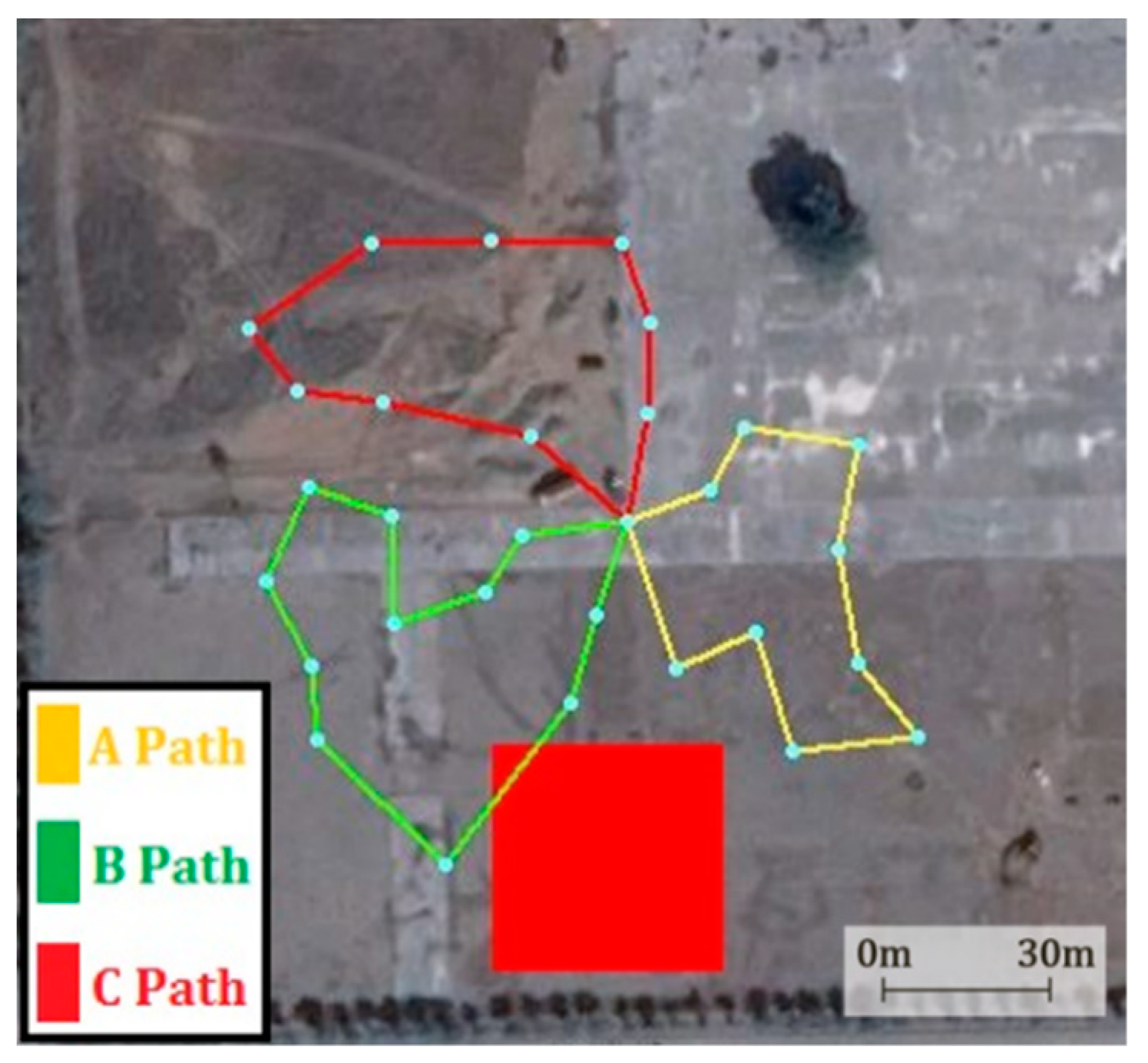
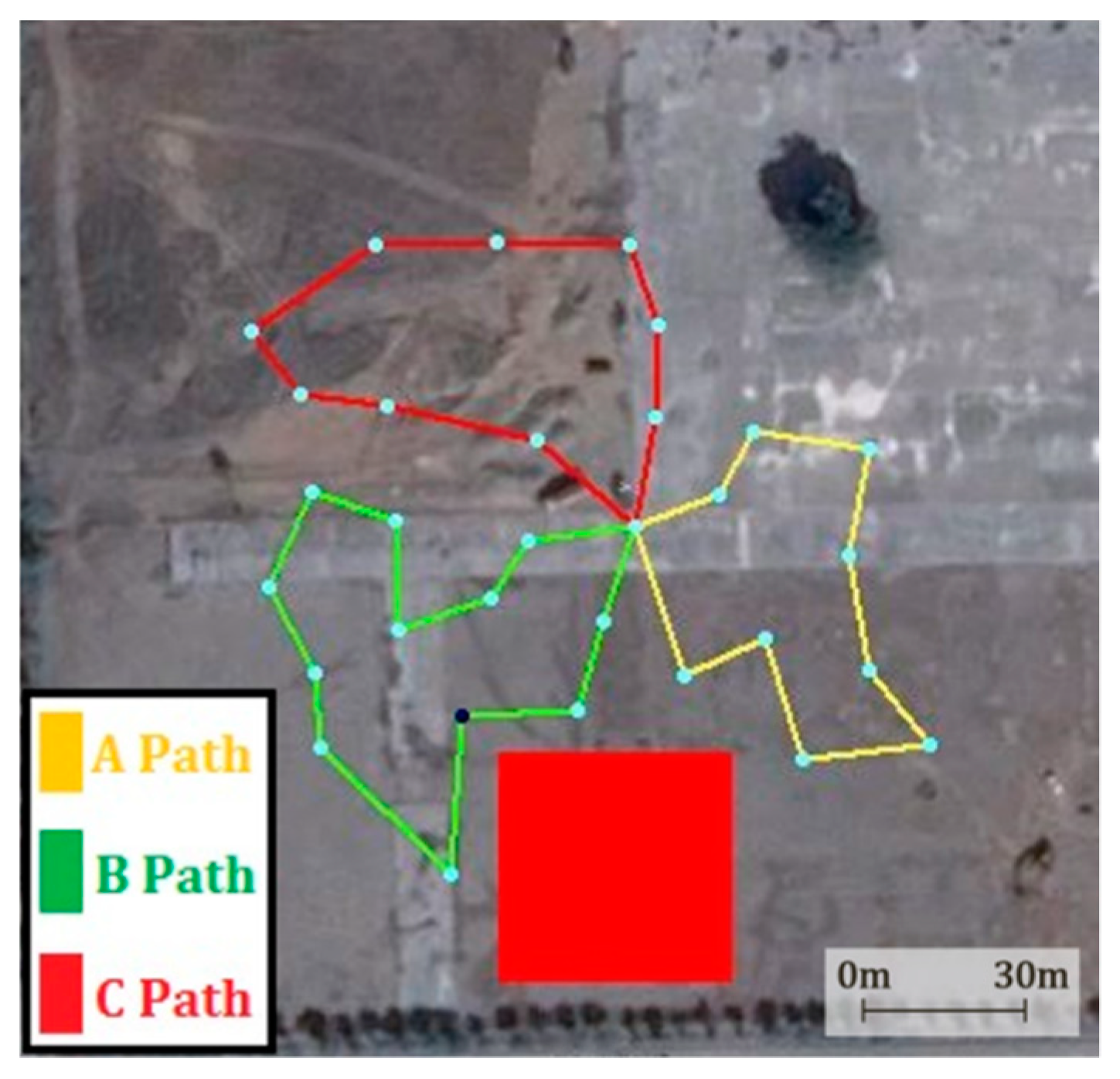
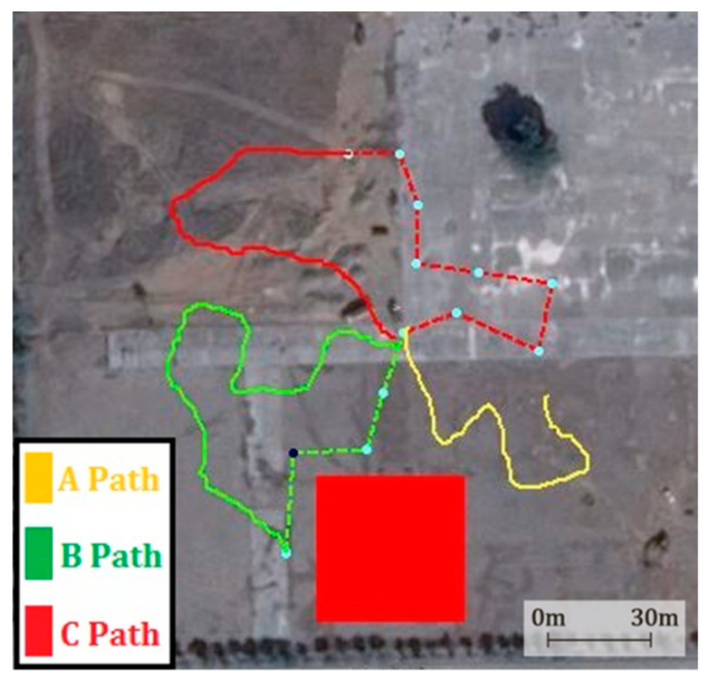
5.3. Tests and Results

This research included several simulations and a full function test. The maximum distance limit by battery capacity was set at 360 m only to fit the largest available size of the pavement field (150 × 150 m) for the experiment, and the shortest total distance paths and the total distance limits for each robot car were set so that they could not exceed these limitations (set as: ITL = 30, ISC = 50, IRTL = 30, CRTL = 30 IRSC = 50, CRSC = 50, and TSC = 2). After all these settings were completed, the paths were dispatched to the robot cars to make them run on their assigned optimum paths.
Figure 18; Figure 19 illustrate ideal paths generated by the algorithm to demonstrate the efficacy considering the “no-travel zone avoidance” function before real field experiments. The test began by randomly setting 30 target points that vehicles must visit and setting a no-travel zone marked as a red rectangle. It was assumed that the battery could only provide a maximum distance limit of 360 m for each car. As shown in Figure 18, the system automatically programed and then dispatched three routes using the 2TS+2OP algorithm without considering the no-travel zone. Consequently, the A path was 194.1 m, the B path was 236.2 m, the C path was 203.9 m, the shortest total distance path was 634.2 m, and the CPU time was 2.77 s.
Although none of the paths exceeded the maximum distance limit, the no-travel zone was touched by the B path. This issue can be solved by the improved no-travel zone algorithm of the next test. In Figure 18, the turning points generated for this case are indicated by the light-blue dots. As the test result, the A path was 194.1 m, the B path was 248.3 m, the C path was 203.9 m, the total distance path was 646.3 m, and the CPU time was 2.54 s. None of the paths exceeded the battery’s maximum distance limit (360 m), and all paths successfully bypassed the no-travel zone.
The next test was an actual full function field test (included path programming, no-travel zone avoidance, and failure complementation) run with scratch-build robot cars. In the beginning of this test, the monitoring station automatically dispatched three optimal paths to the robot cars to visit all target points; however, during the mission, Car-A’s battery was intentionally disconnected (at the point shown in Figure 20) to simulate a failure of a car, and the algorithm could reprogram the path so that the companion healthy cars could complete the remaining path successfully. The trajectory (before failure) of each robot car is shown in Figure 19. According to the log, Car-A failed during the mission at 127.1 m. Because the remote monitoring station did not receive the response from Car-A due to its power cut, the monitoring station automatically sent a command to stop all cars and began re-programming. At this point, Car-B had run 187.2 m, while Car-C was arriving at the 144.8 m mark, and failed Car-A had stopped with four targets unvisited. In this case, the unfinished A path was randomly inserted into another path, and path re-programming was immediately conducted to complement the failure. Figure 21 shows that the remaining path of Car-A was rapidly complemented by Car-B. The re-programming CPU time was 0.24 s, the B Path was 83.9 m, and the C Path was 145.4 m. The remaining paths were re-allocated to Car -B and Car-C to complete the task. The actual distance that Car-B ran after the failure was 90.9 m, while Car-C ran 150.2 m. In total, 241.1 m were run after the failure. The actual trajectory of each robot car in this experiment is shown in Figure 22.
For the final step, the individual distances run by each car (Car A: 127.1 m, Car B: 271.1 m, and Car C: 290.2 m) were obtained, and it was found that none exceeded the maximum distance limit (360 m). The total distance run by the three cars was 688.4 m.

6. Conclusions

In this research, a MAS was successfully developed and an improved algorithm was designed, which combined the A* search and the two-phased Tabu algorithm for multi-vehicle path programming. The programmed paths were able to bypass the no-travel zone by adopting the A* search and to optimize path scheduling by implementing the two-phased TS. Any viable solution could be modified and gradually converged by the improved TS, even if the initial solution exceeded the maximum distance limit.
In the final phase of this research, multiple robot cars were dispatched in a test field to complete multi-waypoint, long-range tasks, which is far beyond a single robot car’s endurance capability. This experiment successfully validated the effectiveness of multi-robot vehicles using the improved 2TS+2OPT algorithm to solve MTRP under the maximum distance limit (such as battery capacity). The experimental results showed that each target point was indeed visited by one of the robot cars without touching the no-travel zone. If any car failed in the middle of the task, the monitoring station reprogrammed the path automatically to re-assign the other healthy cars to complete the remaining path without exceeding the maximum distance limitation.
Multi-robot systems have recently attracted attention from roboticists due to the possibility of accomplishing a task that a single robot cannot. However, this also puts additional burden in setting up or deploying such systems as they can crash with higher probability during cooperation in harsh conditions. This research would provide essential capabilities to multi-robot system’s automation.

Author Contributions

Conceptualization, M.-T.L.; Formal analysis, B.-Y.C. and W.-C.L.; Methodology, M.-T.L.; Project administration, M.-T.L.; Software, B.-Y.C.; Writing—original draft, B.-Y.C.; Writing—review & editing, M.-T.L. and W.-C.L.

Funding

This research was funded by the Ministry of Science and Technology, Taiwan (ROC), grant number MOST 106-2221-E-150-028.

Conflicts of Interest

The authors declare no conflict of interest.

References

  1. Luan, Y.; Xue, H.; Song, B. The Simulation of the Human-Machine Partnership in UCAV Operation. In Proceedings of the 26th International Congress of the Aeronautical Sciences, Anchorage, AK, USA, 14–19 September 2008. [Google Scholar]
  2. Cai, B. Path Programming for Autonomous Unmanned Vehicle System. Bachelor’s Thesis, National Formosa University (NFU), Yunlin, Taiwan, 2015. [Google Scholar]
  3. Tsai, P.; Lin, Y.; Chou, L. Combining corner detection and Dijkstra algorithm for shortest path search and application. J. China Inst. Technol. 2008, 38, 65–83. [Google Scholar]
  4. Hart, P.; Nilsson, N.; Raphael, B. A formal basic for the heuristic determination of minimum cost paths. IEEE Trans. Syst. Cybern. 1968, 4, 100–107. [Google Scholar] [CrossRef]
  5. Lin, S. A Study of Pathfinding Algorithm in Game AI. Master’s Thesis, Lunghwa University of Science and Technology, Taoyuan, Taiwan, 2013. [Google Scholar]
  6. Xie, S.; Cheng, W. AGV path planning based on smoothing A* algorithm. IJSEA 2015, 6, 21–27. [Google Scholar]
  7. Maity, D.S.; Goswami, S. Multipath data transmission with minimization of congestion using ant colony optimization for MTSP and total queue length. IJLRST 2013, 2, 109–114. [Google Scholar]
  8. Sariel-Talay, S.; Balch, T.R.; Erdogan, N. Multiple traveling robot problem: A solution based on dynamic task selection and robust execution. IEEE/ASME Trans. Mechatron. 2009, 14, 198–206. [Google Scholar] [CrossRef]
  9. Yousefikhoshbakht, M.; Didehvar, F.; Rahmati, F. Modification of the ant colony optimization for solving the multiple traveling salesman problem. ROMJIST 2013, 16, 65–80. [Google Scholar]
  10. Necula, R.; Breaban, M.; Raschip, M. Performance Evaluation of Ant Colony System for the Single-Depot Multiple Traveling Salesman Problem. In Proceedings of the 10th International Conference on Hybrid Artificial Intelligence Systems, Bilbao, Spain, 22–24 June 2015; pp. 257–268. [Google Scholar]
  11. Xu, M.; Li, S.; Guo, J. Optimization of Multiple Traveling Salesman Problem Based on Simulated Annealing Genetic Algorithm. In Proceedings of the MATEC Web of Conferences 100, Zhengzhou, China, 20–21 April 2017. [Google Scholar]
  12. Côté, J.F.; Potvin, J.Y. A Tabu search heuristic for the vehicle routing problem with private fleet and common carrier. EJOR 2009, 198, 464–469. [Google Scholar] [CrossRef]
  13. Liao, T.; Huang, W. A study of dynamic logistics based on two-phased method. IJAIT 2008, 2, 76–94. [Google Scholar]
  14. Khamis, A.; Hussein, A.; Elmogy, A. Multi-robot task allocation: A review of the state-of-the-art. In Cooperative Robots and Sensor Networks 2015; Springer: Berlin, Germany, 2015; pp. 31–51. [Google Scholar]
  15. Balch, T.R. Social Entropy: A New Metric for Learning Multi-Robot Teams. In Proceedings of the 10th International FLAIRS Conference (FLAIRS-97), Daytona Beach, FL, USA, 12–14 May 1997; pp. 362–366. [Google Scholar]
  16. Bektas, T. The multiple traveling salesman problem: An overview of formulations and solution procedures. Omega 2006, 34, 209–219. [Google Scholar] [CrossRef]
  17. Hung, F. Vehicle Routing Problem of Integrated Supply Medical Materials in Strategic Alliance Hospitals: A Study of One Medical Center. Bachelor’s Thesis, National Yunlin University of Science and Technology, Yunlin, Taiwan, 2004. [Google Scholar]
  18. Lin, S. Computer solutions of the traveling salesman problem. BSTJ 1965, 44, 2245–2269. [Google Scholar] [CrossRef]
Figure 1. Schematic diagram of the multiple traveling salesman problem (MTSP).
Applsci 09 03756 g001
Figure 2. The full system.
Applsci 09 03756 g002
Figure 3. The system architecture.
Applsci 09 03756 g003
Figure 4. Architecture diagram of the sub-system of a robot car.
Applsci 09 03756 g004
Figure 5. Experimental robot car.
Applsci 09 03756 g005
Figure 6. The 2-opt in-route swap concept.
Applsci 09 03756 g006
Figure 7. The 2-opt swap method concept.
Applsci 09 03756 g007
Figure 8. Main flow chart.
Applsci 09 03756 g008
Figure 9. Schematic diagram of the turning points.
Applsci 09 03756 g009
Figure 10. Schematic diagram of avoiding the no-travel zone.
Applsci 09 03756 g010
Figure 11. Flowchart of path improvement.
Applsci 09 03756 g011
Figure 12. Flow of path programming for complementing the failed path.
Applsci 09 03756 g012
Figure 13. Path generated for bypassing adjacent no-travel zones.
Applsci 09 03756 g013
Figure 14. Optimal path generated for using one vehicle.
Applsci 09 03756 g014
Figure 15. Optimal path generated for using three vehicles.
Applsci 09 03756 g015
Figure 16. Solution convergence diagram.
Applsci 09 03756 g016
Figure 17. C path fail occurred (Left), and a new optimum path generated for covering remaining target (Right).
Applsci 09 03756 g017
Figure 18. The shortest route programmed by the algorithm without considering the no-travel zone.
Applsci 09 03756 g018
Figure 19. The shortest route programmed by the algorithm considering the no-travel zone.
Applsci 09 03756 g019
Figure 20. Trajectories at the moment Car-A failed (the red circle).
Applsci 09 03756 g020
Figure 21. The new path (two dashed lines) generated by failure complementation.
Applsci 09 03756 g021
Figure 22. Experiment trajectory when the task was accomplished.
Applsci 09 03756 g022
Table 1. Distance comparison of 2TS+2OPT to the other three algorithms.
m (vehicles)234567810
n (nodes)510152025304050
HGA198316456512612692828998
SA1853235567357768219961270
MSAGA193299413474576668778956
2TS+2OPT209291417472509569661784
CPU Time (Sec.)0.120.080.30.51.62.32.76.5
(Core I7 2.4 GHz CPU, 8 GB RAM)

