Intelligent Tennis Robot Based on a Deep Neural Network

Abstract

In this paper, an improved you only look once (YOLOv3) algorithm is proposed to make the detection effect better and improve the performance of a tennis ball detection robot. The depth-separable convolution network is combined with the original YOLOv3 and the residual block is added to extract the features of the object. The feature map output by the residual block is merged with the target detection layer through the shortcut layer to improve the network structure of YOLOv3. Both the original model and the improved model are trained by the same tennis ball data set. The results show that the recall is improved from 67.70% to 75.41% and the precision is 88.33%, which outperforms the original 77.18%. The recognition speed of the model is increased by half and the weight is reduced by half after training. All these features provide a great convenience for the application of the deep neural network in embedded devices. Our goal is that the robot is capable of picking up more tennis balls as soon as possible. Inspired by the maximum clique problem (MCP), the pointer network (Ptr-Net) and backtracking algorithm (BA) are utilized to make the robot find the place with the highest concentration of tennis balls. According to the training results, when the number of tennis balls is less than 45, the accuracy of determining the concentration of tennis balls can be as high as 80%.

1. Introduction

With the rapid progress of science and technology, the living standards of human beings are constantly improving, and the service robot market is booming day by day. This includes the development of sweeping robots and restaurant service robots. However, there are not many service robots for sports, especially tennis service robots, and such robots are still in a rudimentary stage of development. Tennis, as a worldwide sport, has many fans all over the world. However, the scattered tennis balls on the court are difficult to deal with, both during training and during matches. Picking up tennis balls is time-consuming and laborious. Based on these factors, we researched and designed an intelligent tennis robot to satisfy the requirements of tennis players. See details in [1].

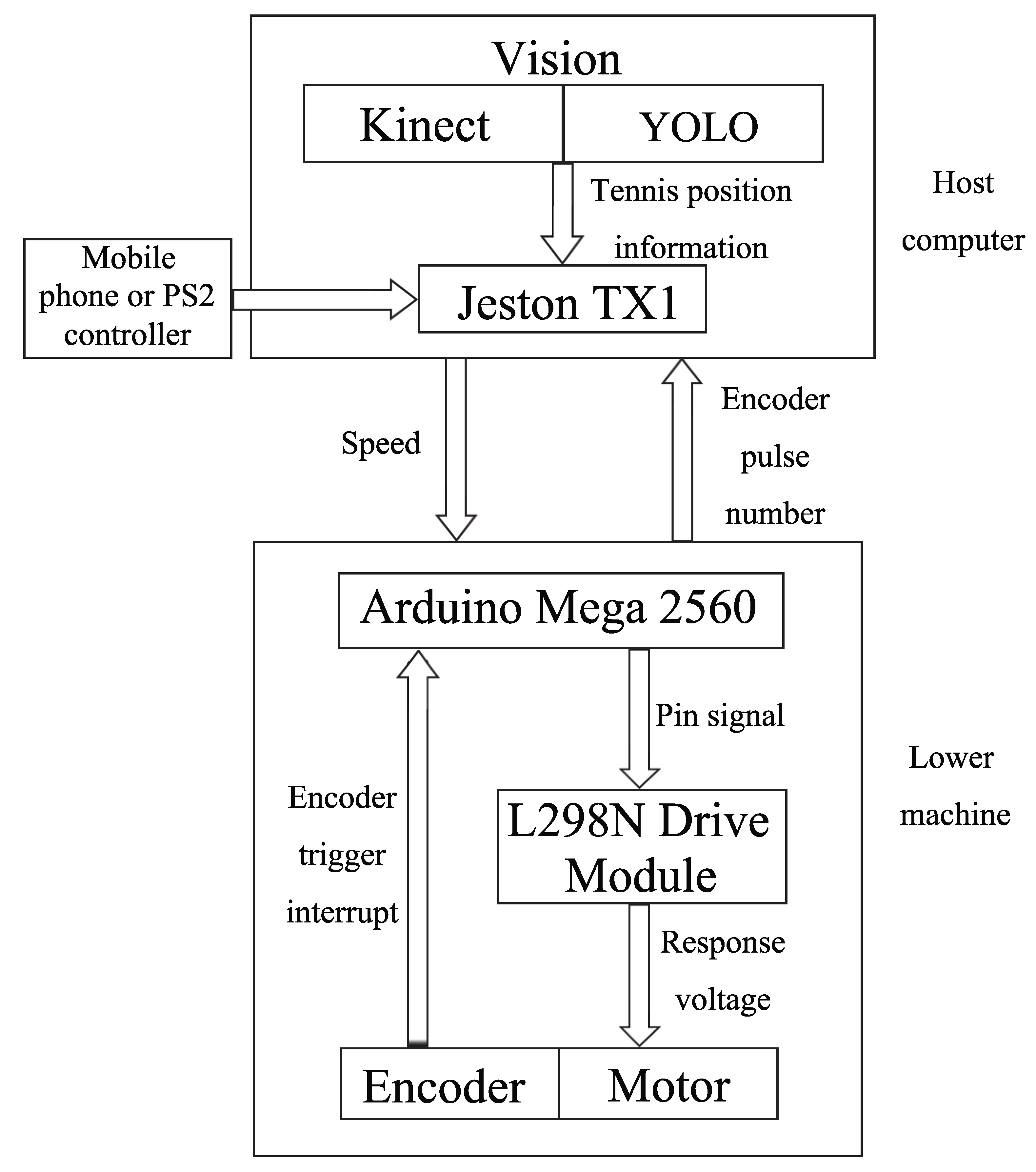
We applied the you only look once (YOLOv3) detection algorithm to design a tennis robot. The structural block diagram of our tennis robot is shown in Figure 1. The tennis robot can be divided into two parts: motion control and machine vision. In the motion control part, we used Arduino Mega 2560 as the control board of the slave computer to drive the DC motor with L298N and count the mileage of the two wheels by the encoder. It forms a closed-loop control system which composes the slave computer. The main function of the slave computer is to receive speed information from the host computer for movement and then feedback to the host. The task of the host computer includes two aspects: Proportional integral derivative (PID) control of the slave computer’s motion and processing of the visual information obtained by Kinect. The robot identifies objects (tennis balls here) by YOLO and then calculates the specific position of the target. We used a laptop or Jeston TX1 as the host computer. Through the unique mechanism of the robot operating system (ROS), communication is established between host computer and the slave computer.

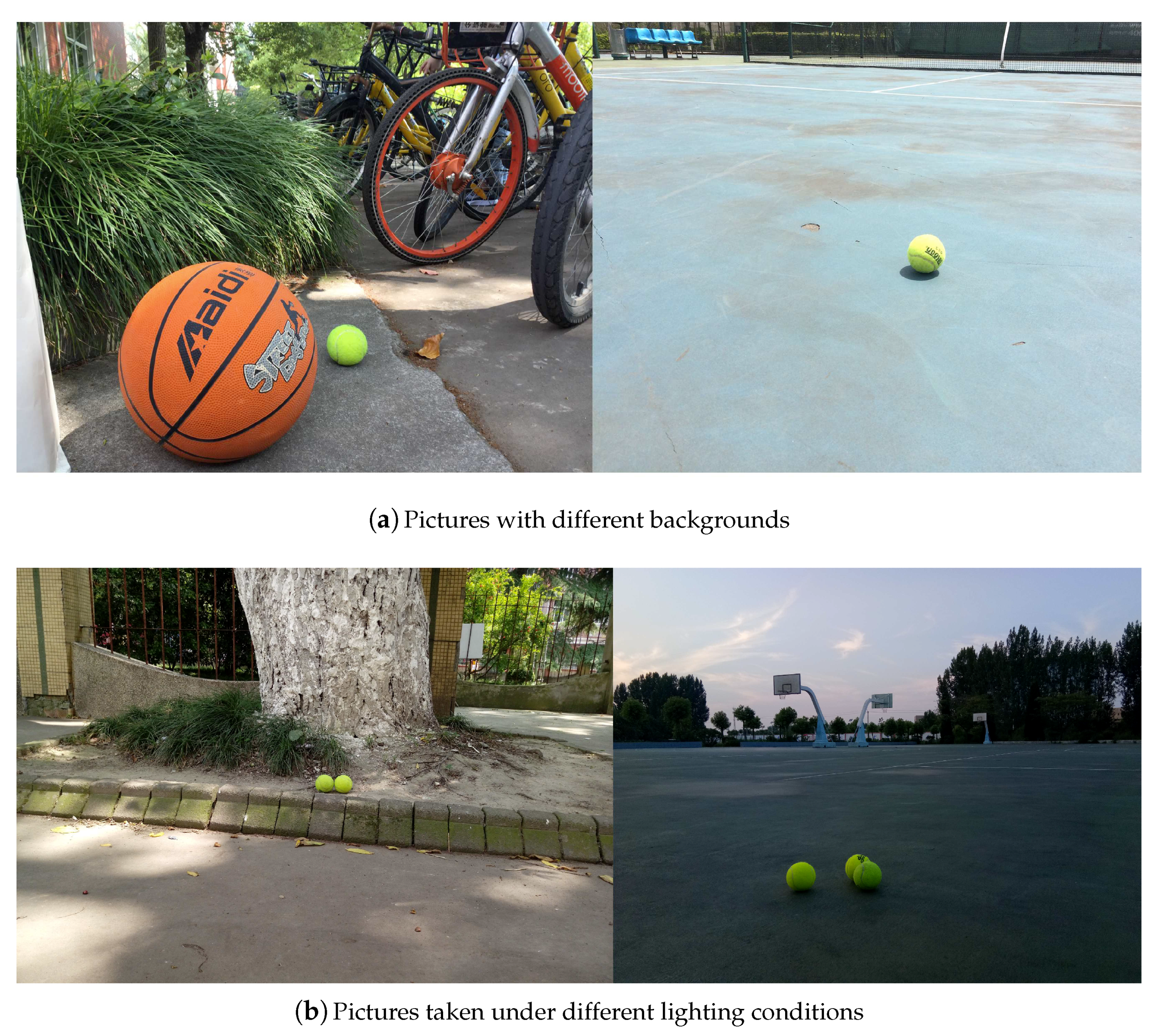
The deep neural network has a very good detection effect and is widely used in the field of target detection. However, many problems need to be considered when deploying the neural network to embedded devices, such as the multiple layers of the network and the huge number of model parameters. Meanwhile, to obtain a better recognition effect, a lot of time needs to be spent training with more data. YOLOv3 extracts features based on the Darknet-53 network, the volume of the convolution calculation is large, the network is deep and complex, and the number of weights is also very large. These features are not conducive to our application to mobile robots. For our usage scenario, we hope that the network model can be better deployed on mobile devices and embedded in development boards. We also hope that it will be lighter and more agile. On the other hand, the deep neural network usually needs to be iterated many times with a large data set to get a good recognition effect. For our research, we only need to recognize tennis balls. Since the images of tennis balls downloaded from the network are usually dissatisfactory, we need to take pictures manually when preparing the data sets, which is time-consuming and labor-intensive. Therefore, we want to only utilize a small number of iterations of mini data sets to train the network model to meet the basic identification requirements.

In our application scenarios, there are usually multiple tennis balls in the picture, and these balls are very likely to overlap. In addition, without the GPU, YOLOv3 detects a picture at a speed of about 12s, which is too slow for a robot. So, we wanted our detection algorithm to not only ensure high accuracy but also work at a faster speed.

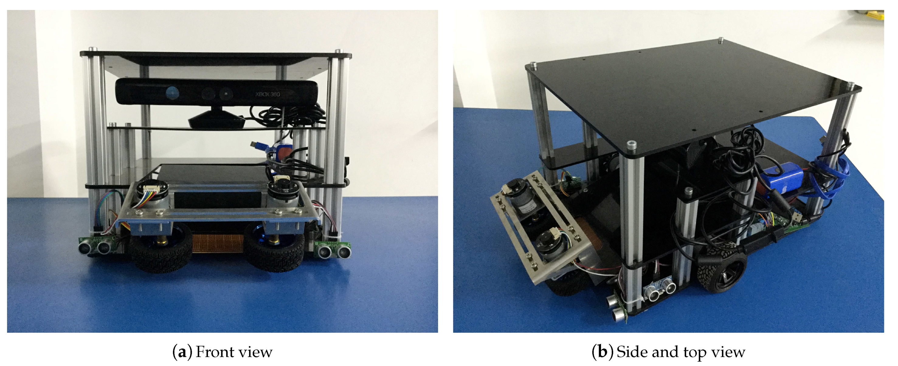
Based on the above factors, we made the following improvements to the YOLOv3 model. Our intelligent tennis robot is shown in Figure 2.

• We replaced the original Darknet-53 with the lightweight network MobileNetv1. We optimized the speed by reducing the number of convolution calculations, model depth, and weights.
• We designed the residual block which can be added to MobileNetv1. For the detection effect, we referred to the idea of the residual block in the DenseNet network and designed a residual block without increasing the network’s burden and depth. We added it to the network structure of MobileNetv1 and then got a good detection effect.

Considering that tennis balls may be scattered everywhere on the tennis court, if our robot can first find the most concentrated place of tennis balls and then identify and pick up tennis balls there, it will save a lot of time and improve efficiency. We drew on the idea of the maximum clique problem (MCP) to solve this problem.

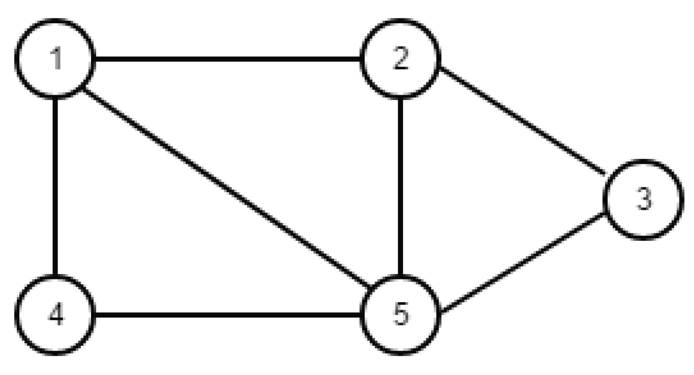
The MCP, also known as the maximum independent set problem, is a classical combinatorial optimization problem in graph theory. It is an important problem in the real world and is widely used in market analysis, scheme selection, signal transmission, computer vision, fault diagnosis, and other fields. The problem can be formally defined as follows: Given an undirected graph $G=(V,E)$, where V is a non-empty set, called a vertex set, E is a set of disordered binary tuples composed of elements in V, called edge sets. In an undirected graph, all disordered pairs of vertices are commonly represented by brackets “()”. If $U\in V$, for any two vertices u and v belonging to U, we can get $(u,v)\in E$. Then, U is a complete subgraph of G. The complete subgraph U of G is the group of G. The largest group of G is the largest complete subgraph of G.

In this paper, we regard each tennis ball scattered on the ground as a point, obtain their position coordinates with the depth camera, and calculate the distances between them. If the distance is less than the average value of the sum of all distances, it is considered that there is a connection between the two tennis balls, so the problem of picking up tennis balls efficiently can be modeled as the maximum clique problem. Under the framework of tensorflow, we use the method of combining the pointer network (Ptr-Net) with the backtracking algorithm (BA) to solve the MCP. After training the Pointer Network, we use the backtracking algorithm to deal with the network output prediction results, which not only reduces the dimensions of the original problem, but also greatly improves the accuracy of the output results. In this way, we can find the gathering point of the tennis balls and pre-process the motion path for the tennis robot.

The chapters of this paper are arranged as follows: firstly, Section 1 introduces the background and significance of this study and briefly introduces the function and principles of our tennis robot. Then, Section 2 briefly introduces YOLO, MobileNet, and ResNet and explains how to combine them to realize the function of tennis detection. Section 3 introduces the solution of MCP based on Ptr-Net and BA and explains how to apply it to the path preprocessing of the tennis robot. Section 4 introduces how to make data sets and compares the training and testing results of different models. It also introduces the training process and results of solving MCP with Ptr-Net and BA. Finally, Section 5 summarizes the work of this paper.

2. Tennis Ball Detection with Improved YOLOv3 Algorithm

With the development of computer vision, a large number of excellent research results have been achieved in the field of object recognition. These results not only have certain theoretical significance, but also have extraordinary practical value, which can provide us with great convenience. In particular, various detection algorithms based on deep learning have replaced the traditional object recognition methods.

Conventional object recognition methods include using a gradient vector histogram (HOG) [2] for pedestrians in a video, using various animal and vehicle detection methods in still images, face recognition using Haar features [3]. These types of traditional identification methods have low recognition rates. They usually take more time to complete the entire recognition process. Additionally, the generalization ability is poor. The emergence of a series of requirements, such as the diversification of recognition objects, diversity of recognition angles, and recognition of background complexity in identification tasks, has brought more challenges to the research of object recognition. Deep learning focuses on studying how to automatically extract multi-layer feature representations from data and uses a series of nonlinear transformations to extract features from raw data in a data-driven manner, avoiding the drawbacks of manual feature extraction. The convolutional neural network (CNN) [4] has been widely and successfully applied to image classification tasks, making it the gold standard for image classification.

Methods based on the convolution neural network can be divided into two categories: one is based on region nomination and the other is based on regression. The regional nomination-based approach is represented by the R-CNN series: R-CNN [5], SPP-Net [6], fast R-CNN [7], and faster R-CNN [8]. Although various improvements have been made, it still adopts the step-by-step detection strategy of first extracting candidate frames and then classifying based on candidate frames. The FPS of the faster R-CNN only reaches seven frames per second (f/s), which is far from reaching real-time requirements. YOLO is a regression-based detection algorithm [9]. It first uses the regression method to directly predict the bounding box coordinates and classification of an object from an image. The detection speed reaches 45 f/s. However, due to the single scale and proportion of the candidate frame selection, the accuracy is reduced when the speed is increased. Redmon J successively proposed the YOLOv2 [10] and YOLOv3 [11] detection algorithms, among which YOLOv3 has a better detection effect. It uses the depth residual network to extract image features and achieves multi-scale prediction, which is implemented on the COCO data set. Additionally, the mAP achieves an effect of 57.9%. In the target detection field, YOLOv3 can ensure accuracy and a detection rate of 51 ms, achieving better detection results.

2.1. Brief Introduction to YOLO

The main idea of YOLO is to use the whole picture as the input of the network, directly returning the position of the bounding box and the category to which the bounding box belongs in the output layer. YOLOv3 is the latest version of YOLO and has many important improvements. In terms of basic image feature extraction, YOLOv3 adopts a network structure called Darknet-53 (containing 53 convolutional layers) instead of using Darknet-19. It draws on the practices of the residual network and sets up shortcut connections between some layers. Besides, tail activation function is also changed from softmax to sigmoid, and the number of anchor boxes is changed from five to three.

The way to implement YOLO is that each grid is predicted to have bounding boxes, and each bounding box is predicted to have a confidence value in addition to its position. This confidence represents the confidence that the predicted box contains the object and the quasi-predictive information of the box prediction. The value is calculated as follows:

$$\mathrm{Pr}\left(\mathrm{Object}\right)\times {\mathrm{IOU}}_{\mathrm{pred}}^{\mathrm{truth}}.$$

(1)

If an object falls in a grid cell, the first item is taken as 1; otherwise, it is given a value of 0. The second item is the value of the predicted bounding box and the actual IoU.

In the test, the class information of each grid prediction is multiplied by the confidence information predicted by the bounding box to obtain the class-specific confidence score for each bounding box:

$$Pr\left({\mathrm{Class}}_i|\mathrm{Object}\right)\times Pr\left(\mathrm{Object}\right)\times {IOU}_{\mathrm{pred}}^{\mathrm{truth}}=Pr\left({\mathrm{Class}}_i\right)\times {\mathrm{IOU}}_{\mathrm{pred}}^{\mathrm{truth}}.$$

(2)

As shown in Equation (2), the product of the category information of each grid prediction and the confidence of each bounding box is the probability that the box belongs to a certain category. After obtaining the class-specific confidence score of each box, the threshold is set and filtered. The boxes with low scores are dropped and non-maximum suppression processing is performed on the reserved boxes to get the final test results.

YOLOv3 applies a residual skip connection to solve the vanishing gradient problem of deep networks and makes use of an up-sampling and concatenation method that preserves fine-grained features for small object detection.

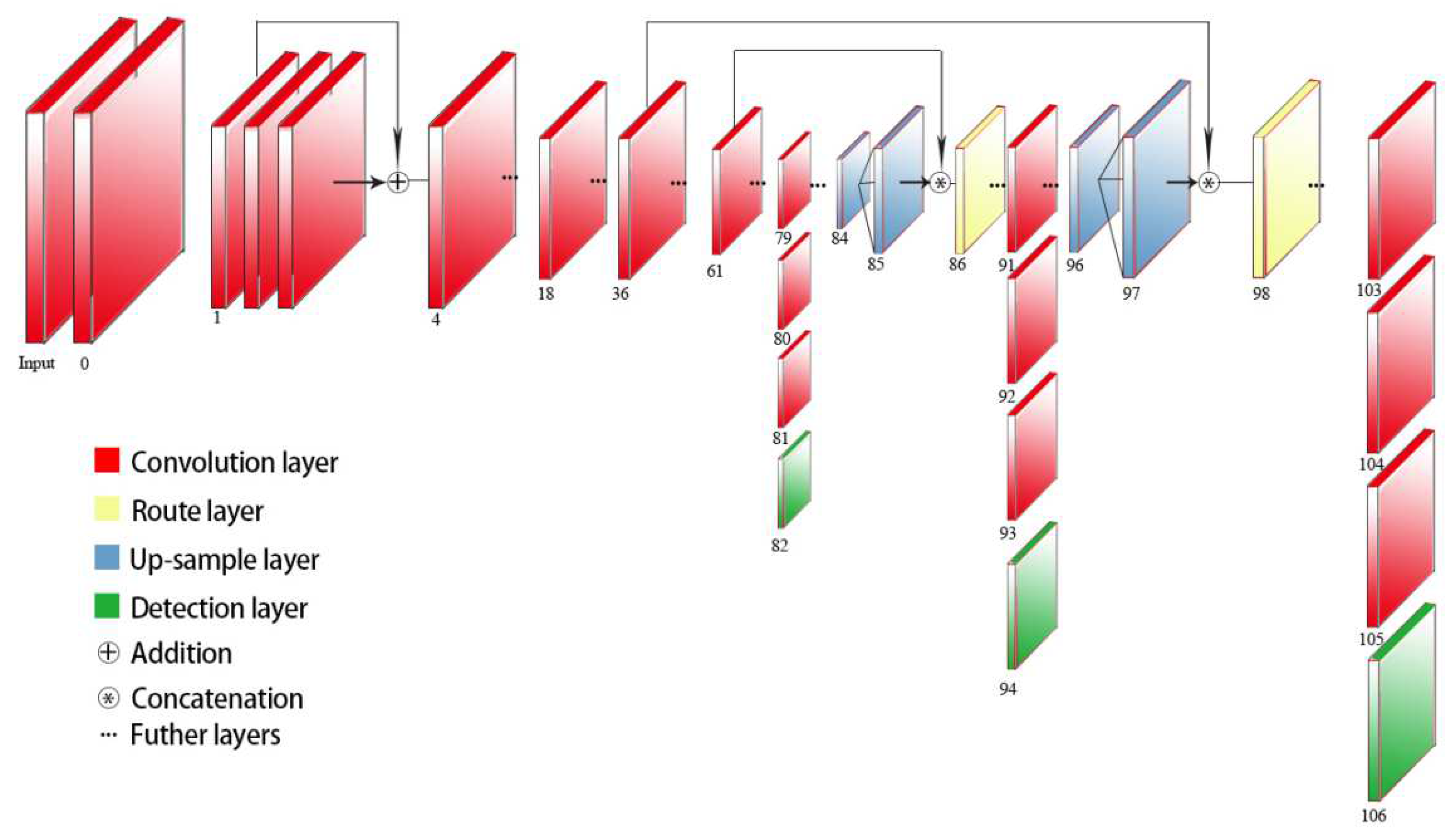
It is well known that YOLOv2 uses pass-through to detect the fine-grained features. However, in YOLOv3, object detection is done using three different scale feature maps. We can see from Figure 3 that after the 79th layer, the measurement result of a scale is obtained through the lower convolutional layers. The feature map used here for detection has 32 times down-sampling compared with the input image. For example, if the input is 416 × 416, the feature map here is 13 × 13. Since the down-sampling factor is high, the receptive field of the feature map is relatively large. Therefore, it is suitable for detecting objects with a relatively large size in the image. In order to achieve fine-grained detection, the feature map of the 79th layer starts to be up-sampled (upstream sampling convolution from the 79th layer to the right) and then merged with the 61st layer feature map, thus obtaining the 91st layer, which is thinner. The feature map of the granularity is also obtained through several convolutional layers to obtain a feature map which is down-sampled 16 times from the input image. It has a medium-scale receptive field and is suitable for detecting medium-scale objects. Then, the 91st layer feature map is again up-sampled and merged with the 36th layer feature map (concatenation). Finally, a feature map of eight down-samplings relative to the input image is obtained. It has the smallest receptive field and is suitable for detecting small objects. In YOLOv3, the k-means algorithm used in YOLOv2 also exists, and nine a priori boxes are clustered to detect objects of different sizes. In addition, for the classification of predicted objects, it is also changed from softmax to logistic, which can support the existence of multiple tags for an object [11].

2.2. Configuration of the Improved Network Structure

In order to solve the problem of the large computational complexity and low computational efficiency of traditional convolution operations, the standard convolution operation in the YOLOv3 model is transformed into a separable convolution operation. We utilize MobileNetv1 instead of Darknet-53 and YOLOv3 to extract features. The latter three resolution grafting networks further detect the possibility, confidence, and categories of targets in each cell. These three resolutions are still 13 × 13, 26 × 26, and 52 × 52, respectively.

However, if we use standard optimization algorithms, such as the gradient descent method, to train a general network or other popular optimization algorithms without these shortcuts or jump connections, we will find that with the deepening of the network, training errors will decrease first and then increase. In theory, the training performance will be better with a deeper theoretical network. However, if there is no residual network, it is more difficult to train a deeper theoretical network with an optimization algorithm. Actually, with the deepening of the network, the number of training errors will increase. So, while simplifying the network, we still consider a joining shortcut. The residual network can map equally through the following two alternatives when the dimensions do not match:

• Add channels directly by zero padding.
• Multiply the W matrix and project it into a new space. The implementation is implemented by 1 × 1 convolution, which directly changes the number of filters of 1 × 1 convolution.

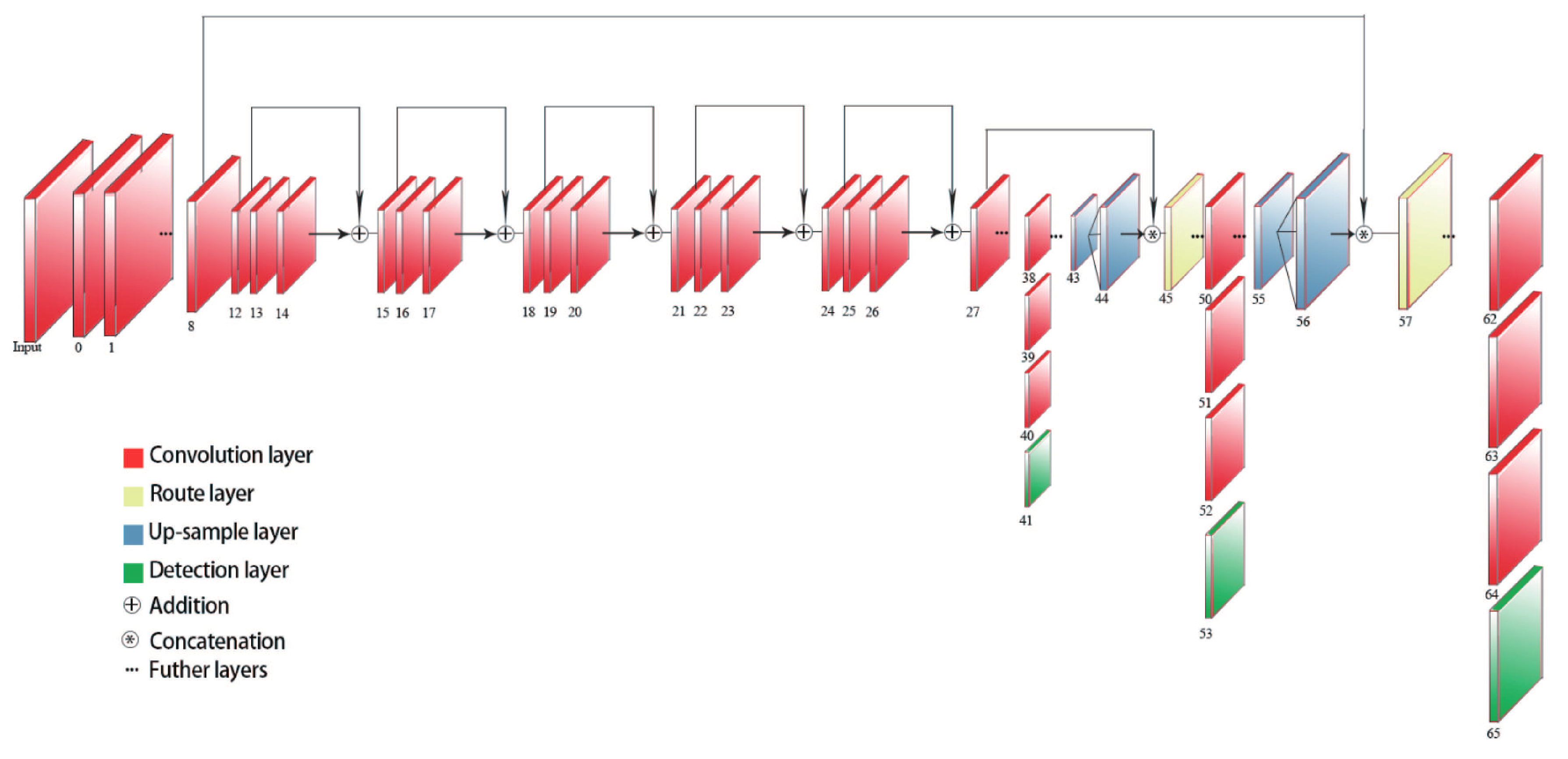
In order not to increase the network burden, we still choose to make a shortcut between the layers of dimension matching. Combined with the network structure of MobileNetv1, the convolution layer is the structure of step two and step one, alternately; the step size of layers 14–23 is one; and five jump connections are added between the 14th layer and the 23rd layer to form a new residual block. The final network structure is shown in Figure 4.

The 8th and 98th layers of the original network are route layers. The reason for this design is that the deep layer network has a good expressive effect. Compared with the deep layer network, the shallow layer network has a better performance. Based on this idea, this paper adjusts the parameters of the original network and retains the route layer.

The main contributions of our improvements are depth-wise separable convolution and residual block. Their principles are given in the following text.

2.2.1. Depth-Wise Separable Convolution

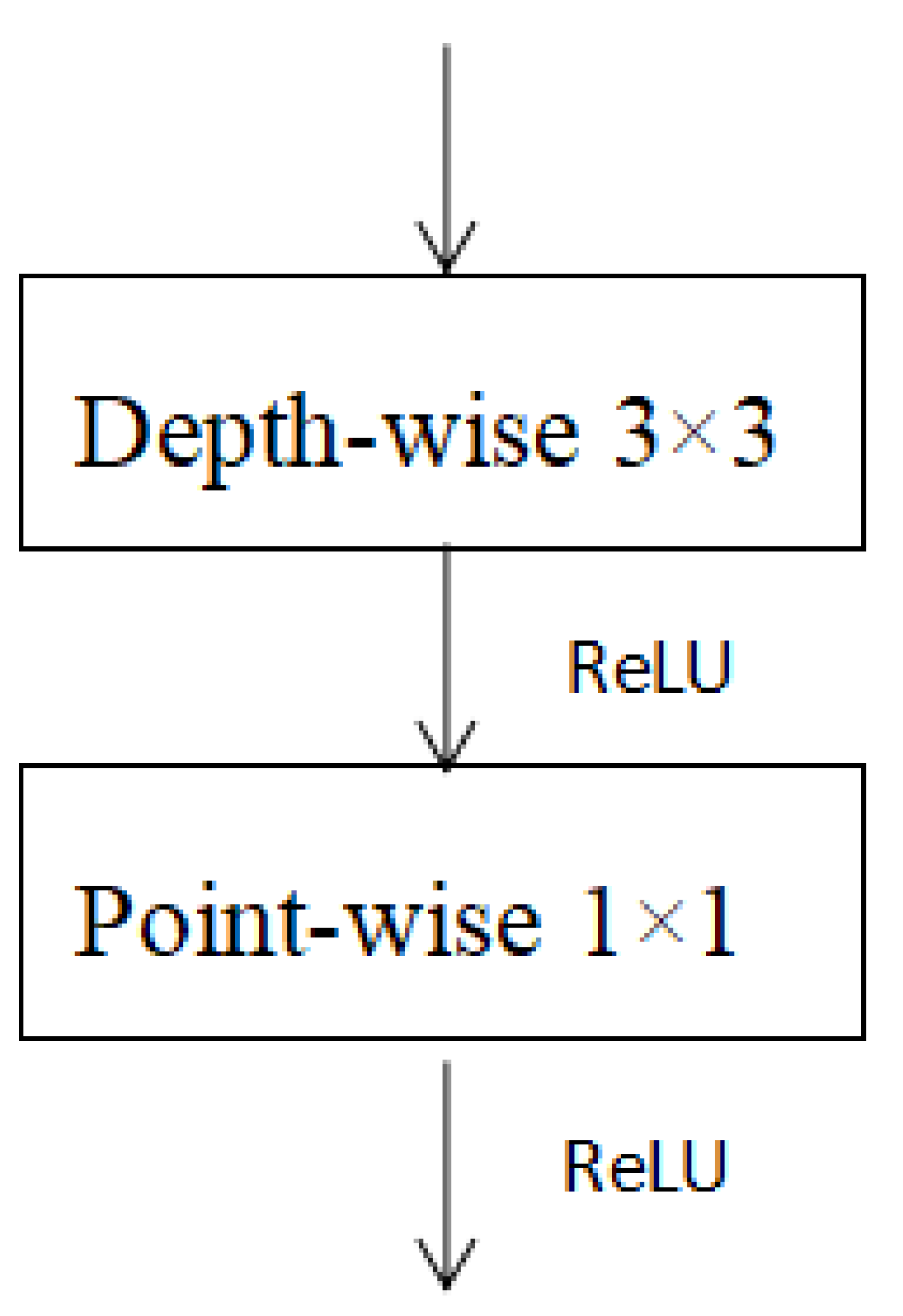
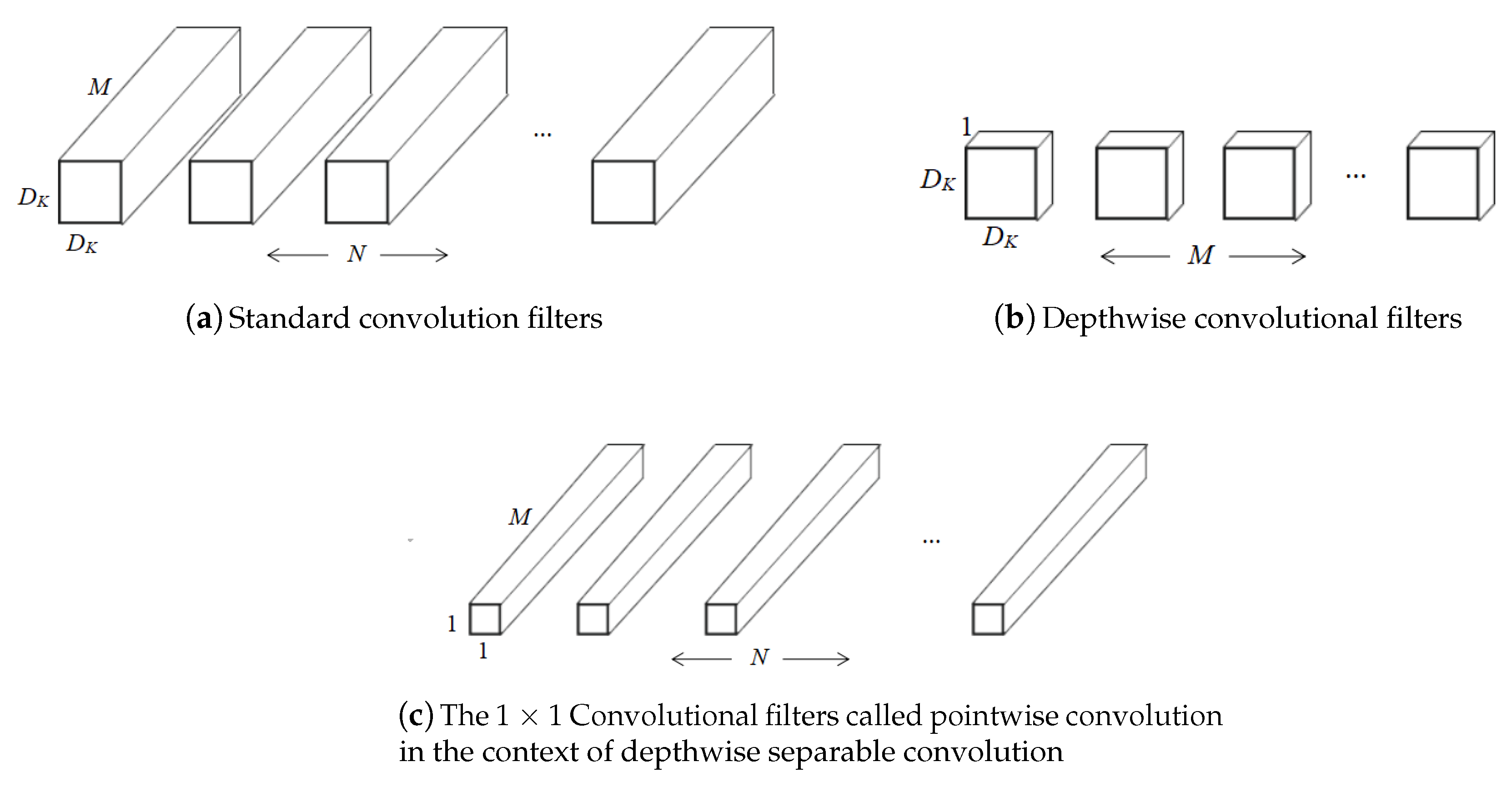
MobileNet is a model that reduces the size of the model and speeds up the inference. Depth-wise (DW) convolution and point-wise (PW) convolution are used to extract features. These two operations are also called depth-wise separable convolution, as shown in Figure 5. The benefit of this is that it is theoretically possible to reduce the time complexity and spatial complexity of the convolutional layer. It can be seen from Equation (3) that since size K of the convolution kernel is usually much smaller than the number of output channels $C_{out}$, the computational complexity of the standard convolution is approximately $K^2$ times that of the combination of DW and PW convolution [12].

$$Complexity=\frac{\text{Depth-wise}\mathrm{Separable}\mathrm{CONV}}{\mathrm{Standard}\mathrm{CONV}}=\frac{1}{K^2}+\frac{1}{C_{\mathrm{out}}}\sim \frac{1}{K^2}.$$

(3)

The main idea is to decompose the traditional volume integral into a depth separable convolution with 1 × 1 convolution. The depth separable convolution means that each channel of the input feature map corresponds to a convolution kernel, so that each channel of the output feature is only related to the channel corresponding to the input feature map. This convolution operation can significantly reduce the size of the model. As shown in Figure 6, for the original convolutional layer, the input feature map has M channels, $D_f$ × $D_f$ is the size of the output feature map, the number of channels is N, and there are N convolution kernels of size $D_k$ × $D_k$. The convolution kernel convolves each feature map of the input, and the convolution calculation of each feature map mainly depends on the size of the generated feature map. Since each pixel of the feature map is output, it is a convolution operation. When the output is $D_f$ × $D_f$, each feature map performs a $D_f$ × $D_f$ convolution operation. The amount of computation per convolution is related to the size of the convolution kernel. Convolution is the matrix multiplication, so the computation is $D_k$ × $D_k$. Then, the calculation required for a convolution kernel is $D_k$ × $D_k$ × $D_f$ × $D_f$ × M. If the number of convolution kernels is N, the total calculation amount is $D_k$ × $D_k$ × $D_f$ × $D_f$ × M × N. For MobileNet’s convolution calculation, when the input is a feature map of M channels, the operation is performed by $D_k$ × $D_k$ convolutions. The output feature map size is $D_f$ × $D_f$, and the operation amount is $D_f$ × $D_f$ × $D_k$ × $D_k$ × M. The number of convolution kernels is the same as that of the input channel, and there is no superimposition between channels, just one-to-one correspondence. In the traditional convolution, M feature maps are superimposed on each other, and all feature map inputs are convolved by N convolution kernels [13].

2.2.2. Resnet

The original network structure of YOLOv3 draws on the idea of the residual network. Darknet-53 goes from layer 0 to layer 74, including 53 convolution layers and 22 res layers. The res layers come from ResNet. When the network layer becomes deeper and deeper, the parameter initialization will generally move close to 0. When the parameters of the shallow network are updated during the training process, it is easy to cause gradient dispersion or the gradient explosion phenomenon, and shallow parameters cannot be updated. This phenomenon is not caused by over-fitting but by the learning parameters of the redundant network layers that are not constantly mapping.

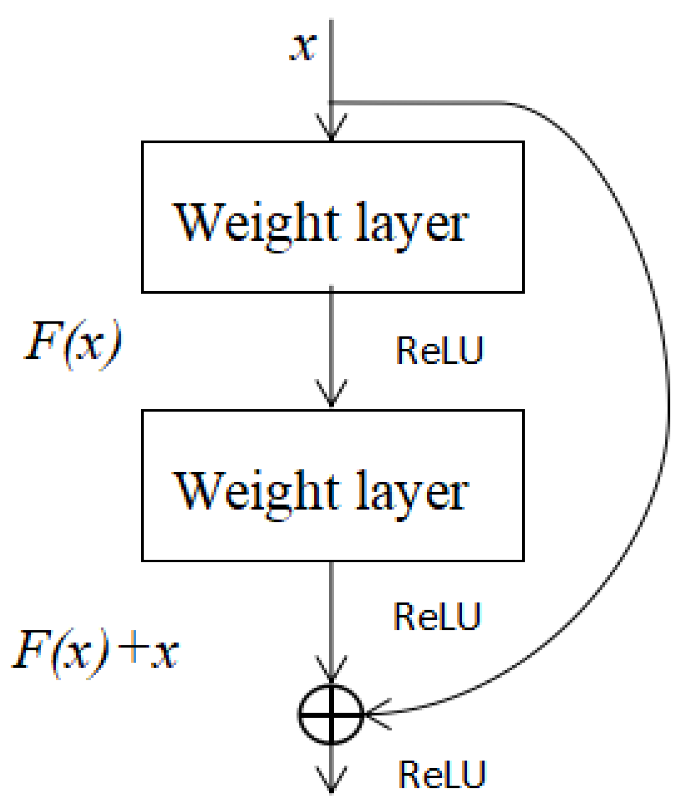
ResNet was jointly proposed by He K and Zhang X in 2015. ResNet takes inspiration from a new idea. If we design a network layer and there is an optimal network level, the designed deep network often has many redundant network layers. Then, we hope that these redundant layers can complete the identity mapping and ensure that the input and output through the identity layer are identical. The identity layer will be judged by the network when training. As shown in Figure 7, it can be seen that x is the input to this layer of residual blocks, also known as the residual of $F\left(x\right)$. x is the input value, and $F\left(x\right)$ is the output after the first layer of linear change and activation. Figure 7 shows that in the residual network, before the second layer is linearly changed and activated, $F\left(x\right)$ adds this layer of input value x, and then activates and outputs. Adding x before the second layer activates the output value. This path is called a shortcut connection. In general, ResNet changes the layer-by-layer training of deep neural networks to phase-by-stage training [14]. The deep neural network is divided into several sub-segments, each of which contains a relatively shallow number of network layers, and then the shortcut connection method is used to make each small segment train the residuals. Each small segment learns a part of the total difference (total loss) and finally reaches an overall smaller loss. It controls the spread of the gradient well, as well as avoids the situation where the gradient disappears or the explosion is not conducive to training [15].

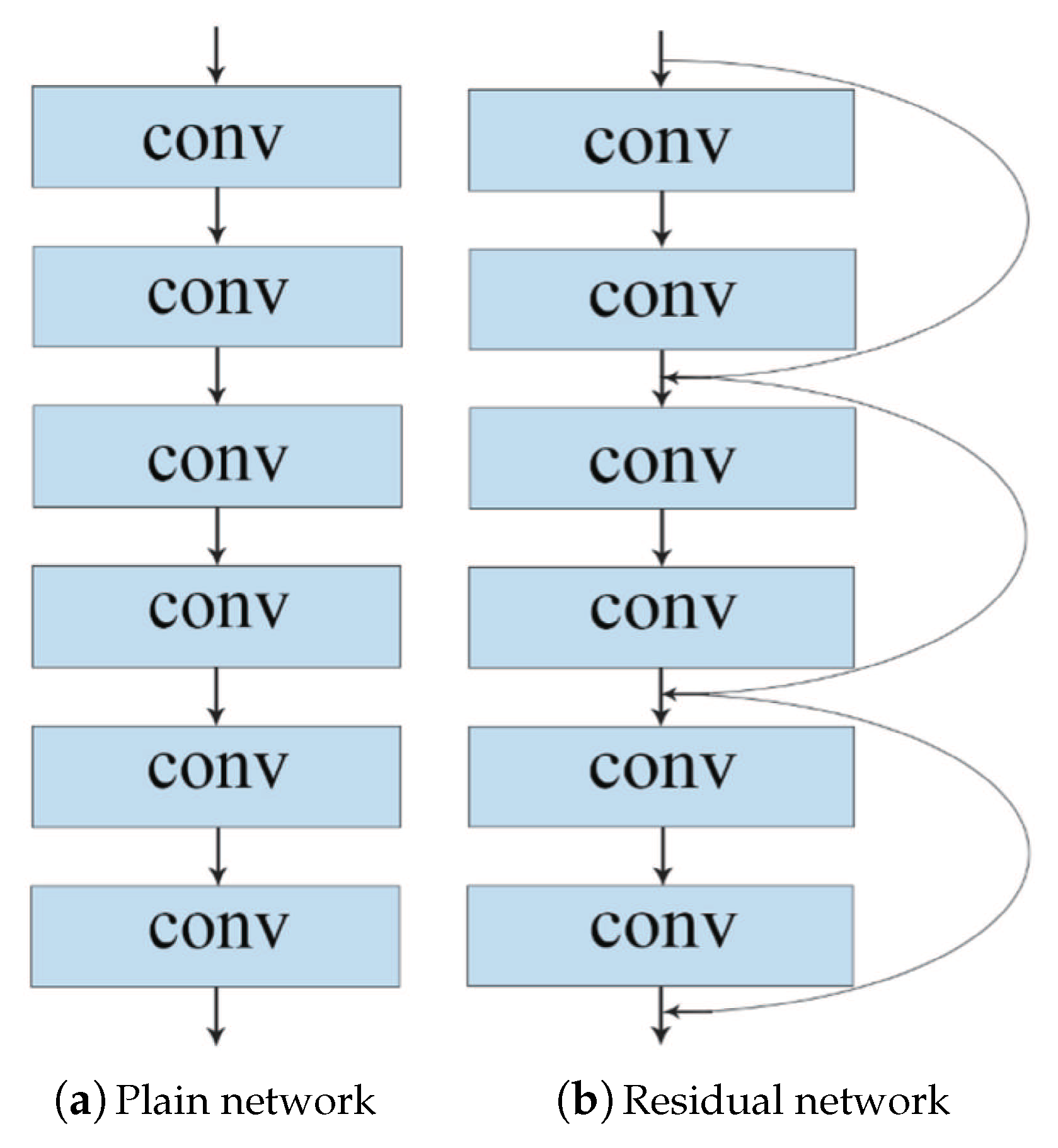
The architectures of the plain network and the residual network are shown in Figure 8. The difference is that, unlike the plain network, ResNet adds all jump connections and adds a shortcut every two layers to form a residual block.

3. Path Preprocessing of the Tennis Robot

After the detection of tennis balls, the improved YOLOv3 algorithm can print labels, confidence, coordinates, and other information on the terminal. The coordinates include x, y, w, and h. x and y represent the coordinates of the central point of the object, and w and h represent the width and height, as shown in Figure 9a. YOLOv3 recognizes the coordinate information of the obtained object and sends it to Kinect to extract the depth information. Kinect can acquire color image and depth information. It can also transform depth image data into the actual depth information of each pixel. According to the imaging principle of the Kinect camera, we can finally get the x, y, and z coordinates in the real world for every tennis ball, as shown in Figure 9b, and calculate the distances between them. Then, we can use the MCP method for path preprocessing.

3.1. Solving the Maximum Clique Problem by the Pointer Network and Backtracking Algorithm

In 1957, Hararv and Ross first proposed the deterministic algorithm for solving the maximum clique problem. Since then, researchers have proposed a variety of deterministic algorithms to solve the MCP. However, with the increase in the complexity of the problem, such as the vertices and edge density, the deterministic algorithm cannot effectively solve these NP-hard problems.

In the late 1980s, researchers began to use heuristic algorithms, such as the sequential greedy heuristic algorithm, genetic algorithm, neural network algorithm and so on, to solve the Maximum Clique Problem and achieved satisfactory results in terms of time performance and results. The only drawback is that it is not always possible to find the global optimal solution. Sometimes, we can only find near optimal values [16].

The main method used in this paper is to combine the backtracking algorithm with the pointer network.

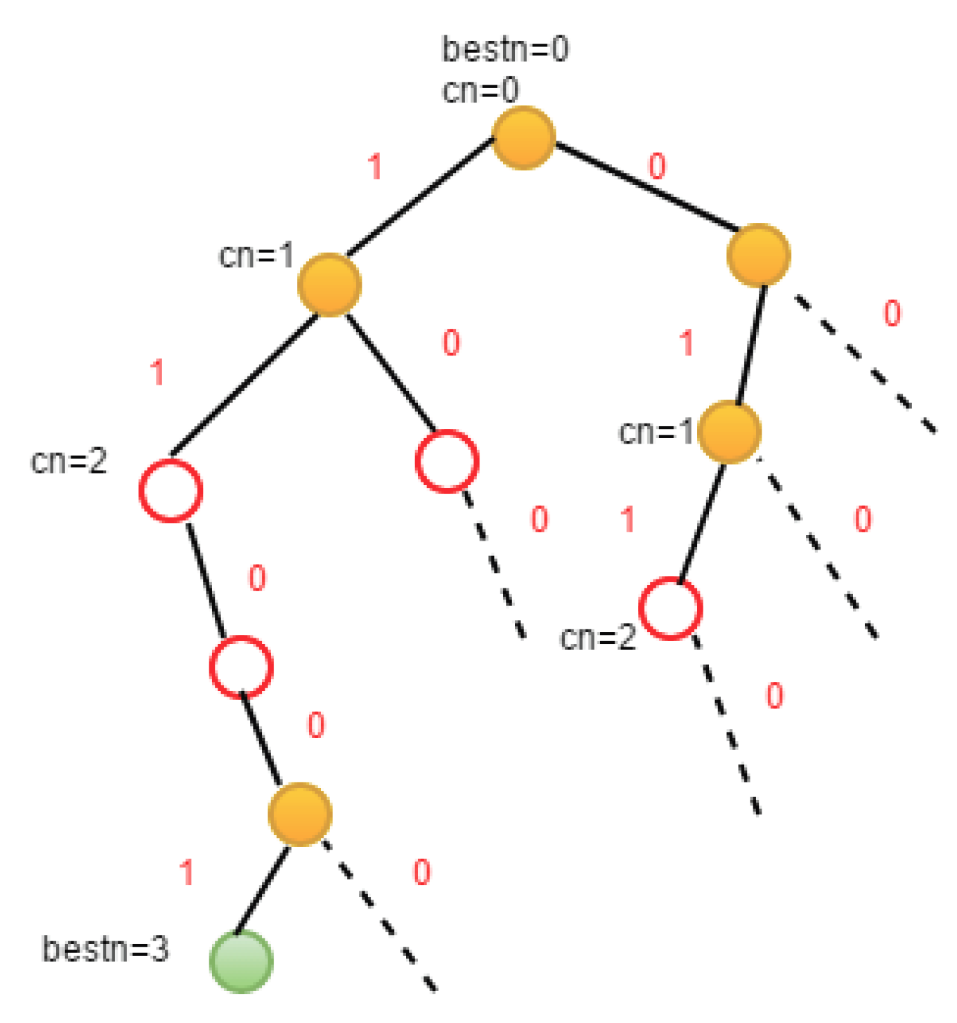
The backtracking algorithm is also known as the “general problem solving method”. It can search for all or any solution of a problem systematically. It is a systematic and jumping search algorithm. This method, based on the root node, traverses the solution space tree according to the depth-first strategy and searches for the solution satisfying the constraints. A process called “pruning” is used to select nodes. When searching for any node in the tree, it first determines whether the corresponding partial solution of the node satisfies the constraint conditions or exceeds the bounds of the objective function. Then, it judges whether the node contains the solution to the problem. If not, it skips the search for the subtree with the node as the root. The search continues along the subtree with the node as its root according to the depth-first strategy.

Pointer networks, referred to as Ptr-Nets, are variants of the attention model and sequence-to-sequence (Seq2seq) model. Instead of converting one sequence into another, they produce a series of pointers to the elements of the input sequence. The most basic usage is to sort elements of variable length sequences or collections. Pointer networks have been widely used to solve combinatorial optimization problems and have achieved good results [17]. For example, Oriol V solved TSP problems in [18] by using a pointer network. Gu S S solved the knapsack problem in [19]. Combining these papers, we find that pointer networks are effective for solving such problems. As a result, we applied them to solve the maximum clique problem in this paper [20].

After training the pointer network, the maximum clique solution given by the network can be obtained. However, since the prediction accuracy of the network is not satisfactory, sometimes, the output result is not a clique or the clique is contained in these nodes. Therefore, we should further use BA to solve the prediction results. In this way, we can not only reduce the dimensions of the original problem but also improve the accuracy of the output results.

3.1.1. Backtracking Algorithm

The basic steps of the Backtracking Algorithm for solving problems are as follows:

• Define the solution space of the problem.
• Determine the structure of the solution space that is easy to search.
• Search for the solution space by the depth-first method, and remove invalid searches with the Pruning function.

Given an undirected graph G, the problem of solving the MCP can be considered as the problem of selecting a subset of the vertex set V of graph G. So, the subset tree can be used to represent the solution space of the problem. The current extension node Z is located at the level i of the solution space tree. Before entering the left subtree, it is necessary to make sure that every vertex from vertex i to the selected vertex set has an edge connection. Before entering the right subtree, you must make sure that there are enough optional vertices to make it possible for the algorithm to find a larger clique in the right subtree.

The graph G is represented by the adjacency matrix, n is the vertex number of G, $cn$ stores the vertex number of the current clique, and $bestn$ stores the vertex number of the largest clique. Also, $cn+n-i$ is the upper bound function that enters the right subtree. When $cn+n-i$ < $bestn$, a larger clique cannot be found in the right subtree. The right node of Z can be cut off by the Pruning function [21].

For the graph shown in Figure 10, this process can be represented by Figure 11.

3.1.2. Architecture of Pointer Networks

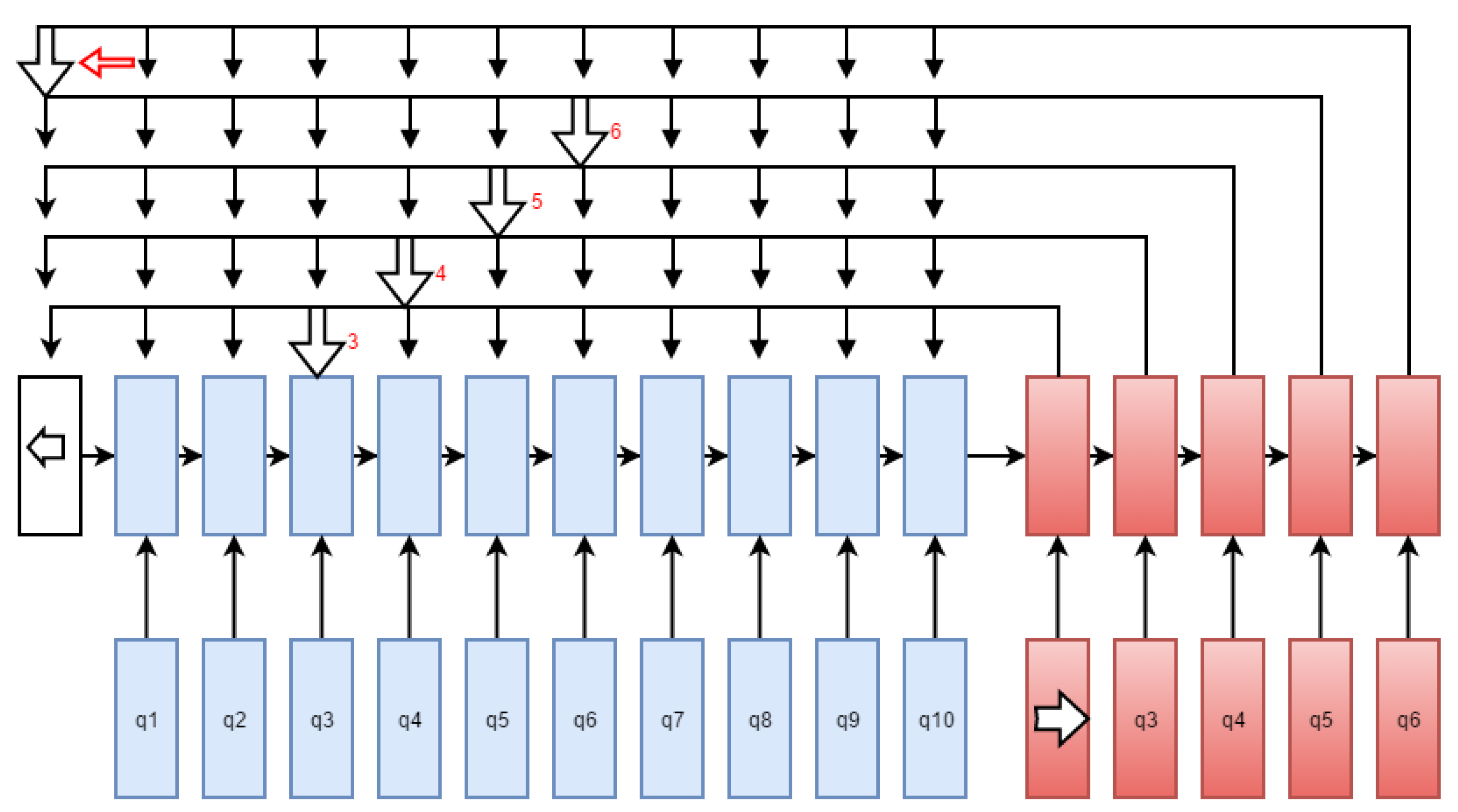
Pointer networks are also Seq2seq models. They are based on an improvement in the attention mechanism that overcomes the “output heavily dependent input” problem in the Seq2seq model. The meaning of “output heavily dependent on input” simply means that the output sequence is selected from the input. For different input sequences, the length of the output sequence depends on the length of the input.

As shown in Figure 10, the method of selecting a point is called pointer. This converts attention into a pointer to select elements in the original input sequence [22]. The attention mechanism learns the weight relationship and the implicit state and then predicts the next output according to them. Ptr-Net directly passes through softmax, pointing to the most likely output element in the input sequence selection.

For the training data set, each line is a piece of data, the input is separated from the output by the word “output”, and the input is a graph represented by a matrix. In the Pointer Network, the model first defines four input parts, which are the input and length of the encoder, the prediction sequence, and the length of the decoder. Then Ptr-Net processes the input and converts it to embedding, which is the same length as the number of hidden neurons in the long short-term memory (LSTM). The solution is to first extend the input and then call the function for 2D convolution. After processing the input, the input shape changes to [batch, max ${}_{-}$ enc ${}_{-}$ seq ${}_{-}$ length, hidden ${}_{-}dim]$ [23]. According to the number of LSTM layers in the configuration, we build the encoder and input the processed input into the model to get the output and the final state of the encoder [24]. After that, we add a start output to the front output, and the start output of the addition will also be the initial input to the encoder, as shown in Figure 12.

Unlike Seq2seq, the input to the Ptr-Net is not the embedding of the target sequence, but the output of the encoder at the corresponding location is based on the value of the target sequence. Similarly, a multi-layer LSTM network is built into the Ptr-Net, where we enter only one value for each batch for each decoder and then loop through the entire decoder process. In the Ptr-Net, two arrays are defined to hold the output sequence and softmax values for each output.

3.2. The Combination of Backtracking Algorithm and Pointer Networks

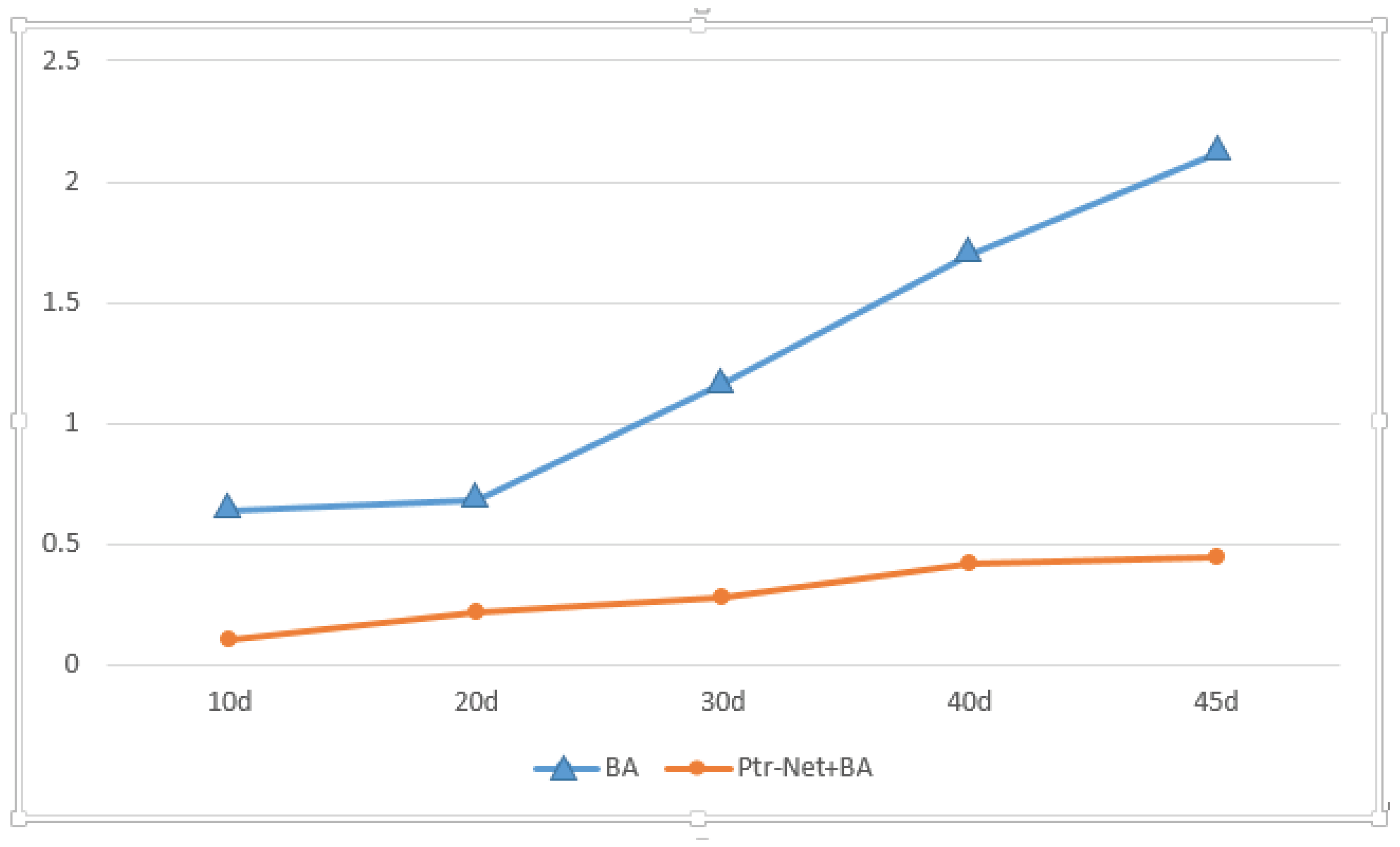
At first, we train the Ptr-Net to only get the solution to the MCP. We find that the accuracy is not so satisfactory. After comparing the predicted answers and the optimal values of the Ptr-Net, we find that the difference between them is not great. The output of the Ptr-Net very likely contains the largest group.

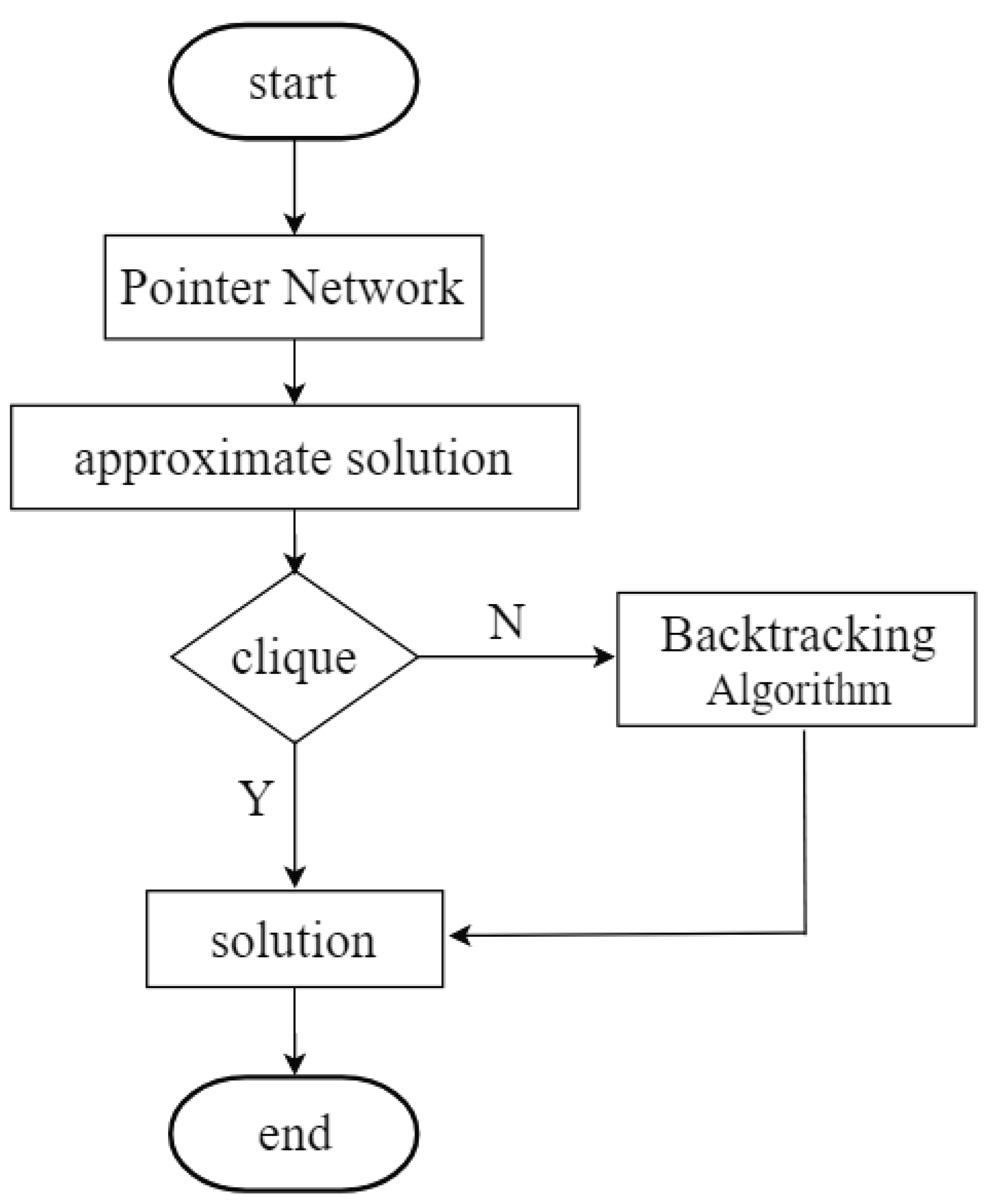
So, we use a method that combines the Ptr-Net with BA. After the Ptr-Net predicts the answer, a judgment is made on the result. If the output result is the optimal value of MCP, it is printed out directly. If not, the maximum clique is continuously found in the predicted selected points by the BA method. The flow chart is shown in Figure 13.

4. Experimental Results and Analysis

4.1. The Experiment of Tennis Ball Detection

4.1.1. Making the Tennis Ball Data Set

Our purpose was to make an intelligent robot that can automatically locate and pick up tennis balls. Because the perspective of the robot is different from that of human beings and the shape of the tennis balls is relatively singular, we did not use online tennis ball pictures to make data sets, but rather, used a manual shooting method. In the process of production, we changed the background, light, and angle and also the number of tennis balls on a picture to make the robot adapt to the situation of multiple tennis ball recognition. At the same time, the training model correctly distinguished tennis balls from other similar objects by using circular objects such as basketballs as the background. The Label Image tool was used to make label files for the data sets and to train data sets. We can see some examples of tennis ball data sets in Figure 14.

4.1.2. Experimental Results and Analysis

During the training process, all models were iterated 2000 times by the same data set. The batch was set to 64, and the number of subdivisions was set to 16. The initial learning rate of YOLOv3 was 0.001, and the rate of the other two models was 0.01. The evaluation criteria of the target detection algorithms were mainly divided into the following: Recall, IoU (intersection over union), and Precision. For a specific test set, P (Positive) target represents the detected target and correspondingly, N (negative) represents the non-detected target. T (true) represents the target being detected and the result being correct, and F (false) represents the target not being detected correctly. Thus, after a data set is detected, the following four target results will be generated: TP, FP, TN, and FN. Their meanings are as follows:

• TP (true positive): which should be detected and is detected.
• FP (false positive): which should not be detected but is detected.
• TN (true negative): which should be detected but is not detected.
• FN (false negative): which should not be detected and is not detected.

Recall refers to the percentage of correctly detected samples. The formula for calculating the ratio of total measurements is as follows:

$$R=\frac{TP}{TP+F\mathrm{N}}.$$

(4)

Precision refers to the correct detection of the detected target. The formula for calculating the proportion of the number of measurements is as follows:

$$\mathrm{P}=\frac{TP}{TP+FP}.$$

(5)

The value of IoU can be understood as the coincidence degree between the predicted frame and the marked frame in the original picture. It is a measure of the deviation of single target detection [15].

Figure 15, Figure 16 and Figure 17 provide the IoU and Loss curves of the YOLOv3 algorithm, the YOLOv3 algorithm after adding MobileNet, and the YOLOv3 algorithm with residual block and MobileNet separately.

From the above curves and images, it can be seen that the loss function decreases continuously with training and finally approaches saturation. The final results are all 0.1. Especially for the MobiletNet + ResNet + YOLO model, the final loss function is obviously less than 0.1. The IoU curves show that the improved algorithm can use a bounding box to mark objects in the image well, and the matching degree between the prediction frame and the actual frame is relatively high, which is basically similar to the results of the original YOLOv3 network.

We recorded the Recall, IoU, and precision of three different models with a threshold of 0.5, and also compared their running speeds and weights. The speed was based on the average time required to detect a picture, these two experimental results were compared under different conditions. One was run on a PC with Intel Core i7-7700K CPU and NVIDIA GeForce GTX 1070 GPU, 64-bit operating system. The other was run on a laptop with Intel Core i5-6200U CPU, 64-bit operating system without GPU.

Table 1. Performance comparison.

	Recall	IoU	Precision	Detection Speed(GPU/CPU) (s)	Weight (M)
YOLO	67.70%	93.19%	77.18%	0.0322/12.59	246.3
MobileNet + YOLO	75.22%	87.48%	83.91%	0.0160/6.46	138.6
MobileNet + ResNet + YOLO	75.41%	88.95%	88.33%	0.0163/6.13	138.7

shows that the biggest advantage of the improved algorithm is that its speed is about twice as fast as that of the original YOLOv3 algorithm, and the size of the model is reduced by half. Although the training parameters are reduced, the Precision of the model described in this paper is also greater than that of the original YOLOv3 model.

We compared the detection results of different lighting conditions using our improved model (MobileNet + ResNet + YOLOv3). There are three main situations:

• Good outdoor light;
• Dim background, such as a cloudy day or sunset;
• Artificial lighting.

The examples of the test data sets are shown in Figure 18.

The precision of these three situations was 88.33%, 62.97%, and 77.78%. From Figure 18c, we can see that in the case of dim light, the detection effect will become worse. If the light is very dim, even tennis balls can not be detected. However, the presence of artificial light sources with good illumination has little influence on the detection results. From these results, we can see that the detection network needs good lighting conditions. In the case of clear illumination, the artificial light has little influence on the detection results.

We also see that after training, the model can be well adapted to different detection environments and backgrounds. In the presence of multiple tennis balls, it can still accurately locate each tennis ball and obtain great detection results.

4.2. Experiment of the Solving Maximum Clique Problem

4.2.1. Data Structure and Generation of The MCP

In order to facilitate Ptr-Net training, we used a symmetric matrix to represent the connections among vertices: “1” represents an edge connection between two vertices, “0” represents no connection. According to this method, the graph shown in Figure 10 can be represented by the matrix shown below:

$$\begin{array}{c}\hfill \left[\begin{array}{ccccc}0& 1& 0& 1& 1\\ 1& 0& 1& 0& 1\\ 0& 1& 0& 0& 1\\ 1& 0& 0& 0& 1\\ 1& 1& 1& 1& 0\end{array}\right]\end{array}$$

(6)

When making training data sets and test data sets, the input matrix is separated from the answers of maximum cliques by the word “output”.

The steps of data set generation are as follows:

• The random matrix is used to represent the connections among nodes in the graph. At least two points in the graph are connected. When the Matlab program randomly generates the matrix, the probability of the value of each position in the matrix being “1” is more than 0.4.
• One hundred sets of data representing the connections among graphs are generated, and the MCP is solved by the backtracking algorithm method, and the answer obtained is regarded as the optimal value.
• The input matrix and the optimal result are stitched together into the text as the training data set.
• The above three steps are repeated to create the validation data set, which has the same format as the training data set.

Data in five different dimensions (10, 20, 30, 40 and 45) were trained and tested. The training data set and the test data set had one hundred sets of data respectively.

4.2.2. Experimental Results and Analysis

The maximum clique problem for different dimensions was trained at least 70,000 times with one hundred sets of data. Since we used the BA to calculate the optimal value, the corresponding accuracy rate was 100%. The results of the experiment for MCPs with 10, 20, 30, 40, and 45 dimensions are shown in

Table 2. Accuracy of results from different dimensions.

Dimension	Method	Time for 100 Groups (s)	Accuracy
10d	BA	0.636	/
	Ptr-Net + BA	0.107	72.25%
20d	BA	0.684	/
	Ptr-Net + BA	0.219	83.46%
30d	BA	1.166	/
	Ptr-Net + BA	0.282	88.9%
40d	BA	1.700	/
	Ptr-Net + BA	0.418	78.6%
45d	BA	2.120	/
	Ptr-Net + BA	0.447	81.5%

.

In order to evaluate the effect of the training result of the model, “Accuracy” is defined as follows: the sum of the number of points of the maximum clique solved by the model divided by the sum of the number of points contained in the optimal result of the MCP. Its mathematical expression is as follows:

$$\begin{array}{c}\hfill Accuracy=\frac{SumofB}{SumofC}\times 100\%,\end{array}$$

(7)

where B is the output answer after training and C is the optimal result.

It can be seen from the experimental data that the method of combining Ptr-Nets with BA can not only solve the MCP but can also achieve an accuracy level of more than 70% when the dimension is below 50. The performance is acceptable for real applications.

With the information shown in Table 2, we generated the time plots of the two algorithms for solving the MCP, as shown in Figure 19. We can clearly see the advantage of the algorithm in terms of time. For Ptr-Net, the solution of the problem can be calculated in batches after loading the model once. However, for the traditional deterministic algorithm, the total computation time was superimposed according to the amount of input data. As the dimension of the MCP increased, the time required for Ptr-Net increased slowly.

5. Conclusions

This paper used the lightweight network MobileNet with a separable convolution method and added residual blocks. We showed that under the condition that the network structure is reasonable, the redundant network parameters are removed and the operation speed is improved. Finally, the speed is twice as fast as before, and the weight of the network is reduced to half of the original. This will greatly speed up the rate of network model invocation for embedded devices and realize real-time detection. Of course, while improving the speed, we also ensured that the accuracy was satisfactory. In future work, we will continue to explore whether there are other methods to improve the accuracy of single target recognition without expanding the number of calculations required. The improved network will be more suitable for embedded development boards, such as the PYNQ development boards produced by XILINX. We also used the methods of pointer network and backtracking algorithm to pretreat the identified tennis balls, focused on the tennis balls by solving the maximum clique problem, and proved its feasibility through experiments. These results provide a good start for the application of the deep neural network in intelligent robots and hardware devices.