Article

A Statistical Performance Analysis of Named Data Ultra Dense Networks

1
Department of Electronics & Computer Engineering, Hongik University, Sejong City 30016, Korea
2
College of Science and Technology, Hongik University, Sejong City 30016, Korea
3
Department of Software and Communications Engineering, Hongik University, Sejong City 30016, Korea
*
Author to whom correspondence should be addressed.
Appl. Sci. 2019, 9(18), 3714; https://doi.org/10.3390/app9183714
Submission received: 28 June 2019 / Revised: 30 August 2019 / Accepted: 3 September 2019 / Published: 6 September 2019

Abstract

:
Named data networking (NDN) is a novel communication paradigm that employs names rather than references to the location of the content. It exploits in-network caching among different nodes in a network to provide the fast delivery of content. Thus, it reduces the backhaul traffic on the original producer and also eliminates the need for a stable connection between the source (consumer) and destination (producer). However, a bottleneck or congestion may still occur in very crowded areas, such as shopping malls, concerts, or stadiums, where thousands of users are requesting information from a device that resides at the edge of the network. This paper provides an analysis of content delivery in terms of the interest satisfaction rate (ISR) in ultra-dense network traffic situations and presents a final and an adequate statistical model based on multiple linear regression (MLR) to enhance ISR. A four-way factorial design was used to generate the dataset by performing simulations in ndnSIM. The results show that there is no significant interaction between four predictors: number of nodes (NN), number of interests (NI) per second, router bandwidth (RB), and router delay (RD). Moreover, the NI has a negative effect, and log(RB) has a positive effect on the ISR. The NN less than 10 has a significantly higher effect on the ISR compared with other nodes’ densities.

1. Introduction

The proliferation of Internet of Things (IoT) devices along with advances in wireless communication technologies, such as multi-access edge computing (MEC) [1], multiple-input and multiple-output (MIMO) [2], millimeter-wave (MMW) [3], and Fifth Generation (5G) and beyond, offer novel opportunities to support applications (e.g., smart cities [4], intelligent health-care systems [5], autonomous vehicles [6], and the industrial IoT [7]) that are becoming an integral part of our modern life. These smart applications further aid the transformation of IoT from concept to reality. The fourth industrial revolution, which is helping to build smart infrastructures, would not be able to happen without the help of the IoT [8]. The IoT can be a collection of diverse types of device, such as smartphones, daily household electronic equipment, radio frequency identification (RFID) tags, smart gadgets, sensors, and actuators. Connecting these devices to the Internet and human users may result in the production of massive amounts of useful data [9]. Currently, all of these devices employ the location-based transmission control protocol/Internet protocol (TCP/IP) networking model for communication, and they face many issues, as these devices could be numbered in the billions, producing zettabytes of data [10]. Moreover, IoT application users are always more interested in getting updated content rather than the location of that content.
The conventional Internet was designed to share resources and to enable communication among end-to-end hosts, which is called host-oriented communication. However, with the passage of time and technological development, the notion of the Internet has changed. In today’s Internet, a substantial amount of content is uploaded on the Internet from content-oriented applications such as Instagram, Facebook, Twitter, and YouTube. Hence, the content on the Internet is increasing exponentially, and such content needs efficient delivery and retrieval. Therefore, various solutions are provided such as content delivery networks (CDNs) and peer-to-peer (P2P) networks. However, such solutions are based on an end-to-end (host-oriented) architecture, which has many issues and is not a good fit for the contemporary requirements of the Internet such as mobility, security, and latency.
This paradigm shift in user demand and the limitations of the existing Internet architecture motivated researchers to look for an alternative for the future Internet. Named data networking (NDN) [11] is one of the future Internet architectures proposed under the umbrella of information-centric networking (ICN) [12]. It aims to provide an efficient content distribution mechanism in highly dense or congested network environments through its intrinsic property of dealing with content instead of hosts. NDN adopts a pull-based communication model and directly forwards an application layer name at the network layer along the best path to fetch the desired content. In NDN, each node maintains three types of data structure: (1) pending interest table (PIT), (2) content store (CS), and (3) forwarding information base (FIB). A consumer inserts the name of the desired content into an interest packet and forwards it to the network. When an interest arrives at the content router (CR) on its incoming face (the term face/interface is interchangeable and may refer to the physical interface of a router or an application face), the CR first checks the PIT entries to check whether a request for the same name is already in the queue. A single PIT entry maintains in and out records (sub-collections) of each incoming and outgoing interest that has arrived at the router, but has not yet been satisfied. The in-records maintains the incoming face id of an interest packet, whereas the out-records maintain the outgoing face id. If the router has a matching PIT entry, it merely updates the in-records and stores the incoming face information of the current request. However, if the PIT entry does not exist, it checks the CS for the desired content and may respond with the data packet on the interface from where the interest arrives. If desired content is absent from the CS, the router forwards the interest towards the producer using longest prefix matching on the FIB. The FIB data structure can have more than one interface for a single name prefix. Once the interest packet reaches the producer node, it may respond with the data packet, which comprises the name of content, the content itself, and optional fields. When the data packet arrives at the routers, it searches the corresponding PIT entry and forwards the data to all downstream face IDs. Finally, it stores the data in the CS and removes the PIT entry.
It is to be noted that in pure ICN and most of the literature, the CS lookup is the very first operation after the arrival of an interest packet. However, NDN follows the PIT operations first. The main reason behind this logic is to minimize the CS lookup delay because the PIT is considered to be significantly smaller than the CS. The initial implementation of NDN, which was Content Centric-Networking (CCN) also follows the CS lookup operation first. However, the CCN was then extended to the NDN architecture, and NDN is slightly different from CCN in the architectural perspective in a way that in CCN when a content request is received on a content router, then the very first operation is to check the CS. However, NDN checks the PIT at first, and then, the CS is checked [13,14,15,16]. Figure 1 presents the NDN communication process in a network.
NDN routers cache the incoming data based on the name of the content to satisfy future requests with low latency. Thus, they mitigate the backhaul traffic on a single provider. However, in the case of congestion, cache management is a challenging task [17]. Despite the use of caching in the network, a bottleneck may still occur in highly-crowded areas, such as shopping malls, concerts, or stadiums, where thousands of users and IoT devices are requesting information that may change over time (such as dynamic content) [18]. Thus, end users or devices may suffer from a poor packet delivery ratio (PDR). To overcome issues such as cache management, bottleneck mitigation, and congestion, statistical modeling of an ultra-dense network can be utilized to provide a broader view of the network topology and its characteristics.
In this paper, we provide an analysis of content delivery in terms of the interest satisfaction rate (ISR) in ultra-dense network traffic situations. Extensive simulation is carried out in two phases. In the first phase, we ran the simulations in order to select appropriate parameters for our statistical analysis. In the second phase, a four-way factorial design method was employed to generate the dataset for statistical analysis. The rationale of choosing the four-way design method is the higher-level models can be used to reveal the non-linearity of the data, unlike the two- or three-level models, which are used to present the first or second polynomial models. The primary statistical analysis started with the evaluation of the main and interaction effects of predictors and their influence on ISR. A multiple comparison test was conducted to analyze the difference in mean ISR according to the levels of each predictor. In our regression analysis, the initial model includes the candidate predictors with four levels, and their interactions are chosen from the mean plots, interaction plots, and multiple comparison tests. Finally, the best model is selected based on the AIC. Moreover, to validate the accuracy of the final model, residual graphs are employed.
In summary, the contributions of this paper are discussed as follows:
  • We present a four-way factorial design method, which is applied to generate the dataset, including various network parameters, in the ndnSIM simulator.
  • We provide a background and overview of the different statistical analysis methods that can be used to evaluate or enhance the interest satisfaction rate (ISR).
  • We evaluate various network parameters based on mean plots and interaction plots and use multiple comparison tests to analyze how the main effects and interaction effects influence the ISR.
  • We select an adequate multiple linear regression (MLR) model to fit the ISR based on both the Akaike information criterion (AIC) [19] and the coefficient of determination R 2 . A network may achieve a higher ISR in the final model.
The rest of the paper is organized as follows. In Section 2, the motivations of the paper are explained. Section 3 describes the simulation environment and dataset generation method. An overview of different statistical analysis methods is presented in Section 4. The results are presented in Section 5, and finally, the discussion and conclusion are in Section 6 and Section 7, respectively.

2. Motivation: Ultra-Dense Network

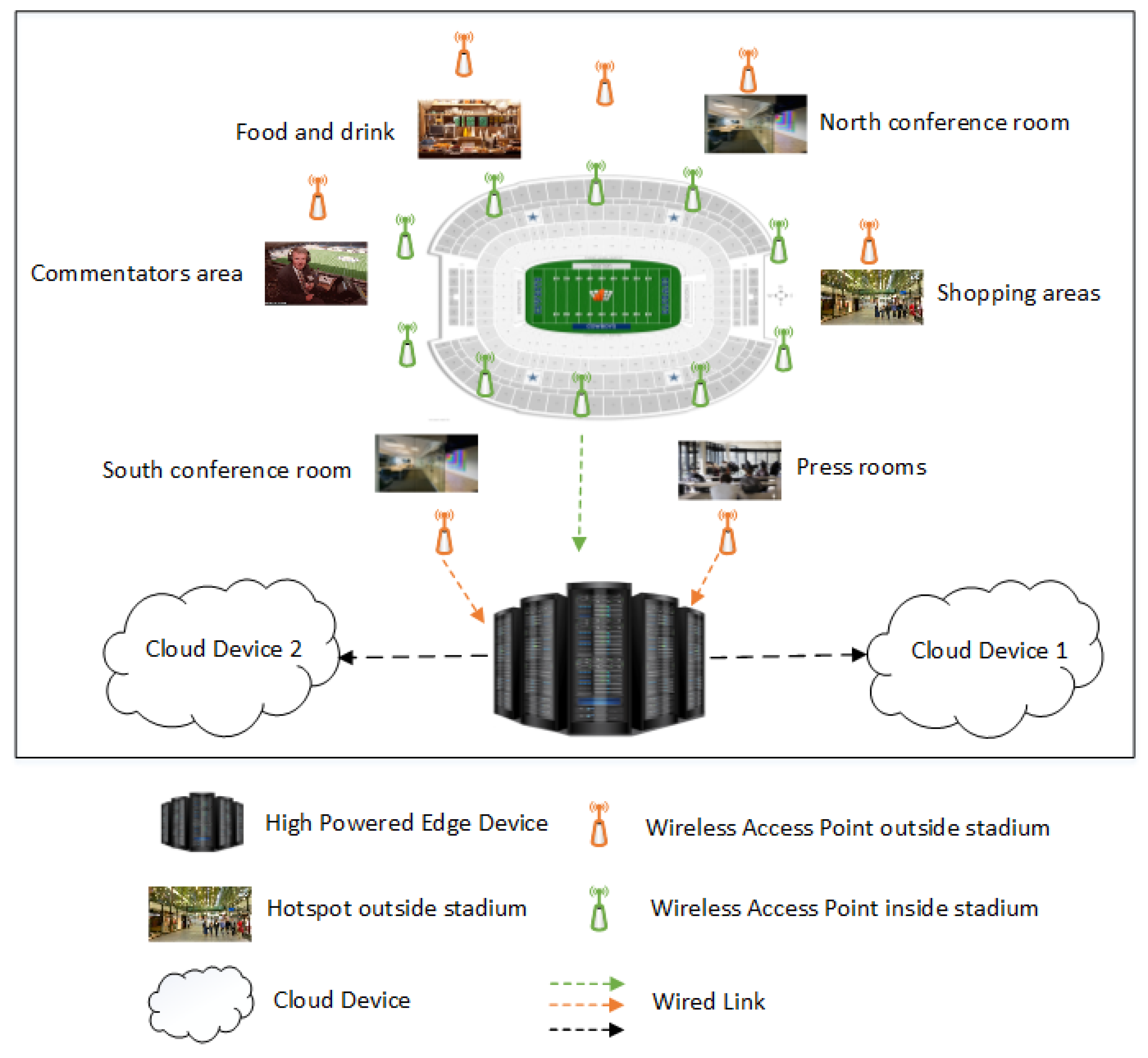
The motivation for this paper can be illustrated by an example shown in Figure 2, which shows a use case scenario for the ultra-dense network environment of a stadium. Generally, a stadium is considered to be a highly-crowded area, where communication may be affected by various factors, such as interference, congestion, and bottlenecks. According to the statistics presented in the case study [20], the largest stadium in the world is Pyongyang, North Korea, with a capacity of 150,000 people, whereas the second largest stadium is in Kolkata, India, with a capacity of 120,000 people. Moreover, as of 2014, 934 stadiums in the world have more than 30,000 seats. However, these numbers may be exceeded, since the hotspot must include those regions that are outside the bowl area, such as conference rooms, press rooms, shopping areas, and restaurants. Stadiums with such a capacity of people make the size and configuration of the network complex, and congestion and interference may often occur. Several conventional design and deployment considerations have been proposed in the literature [18,20]. Some of the design and deployment requirements that have been discussed in the literature so far are:
(1)
Radio frequency (RF) coverage: The RF coverage must be the same throughout the stadium so that the users are not affected by signal fading due to signal attenuation and obstacles.
(2)
Multimedia support: The stadium network must support all service types, such as audio or video streaming [20].
(3)
Real-time and reliable connection: The stadium network should support a real-time and extremely reliable connection so that a cooperative and intelligent communication system can handle emergency scenarios in such a crowded area.
(4)
Hands-off management: Users in the stadium may be mobile and may change their position very often, mainly if they are outside the bowl area. Therefore, reliable hands-off strategies should be established in these areas to avoid intermittent connectivity.
(5)
Interference management: Interference may occur in the stadium due to the deployment of multiple wireless access points (WAP) inside and outside the stadium. Minimizing interference may increase network capacity and throughput.
(6)
Edge computing: A stadium network must be facilitated with the emerging technology of edge computing. Edge computing offers cloud resources closer to the end-users, thereby improving the latency requirements and reducing the backhaul traffic on cloud devices [21].
(7)
Bottleneck mitigation: Ultra-dense networks with single edge computing devices are cost efficient. However, bottleneck or congestion may occur [22], since many WAPs may frequently and directly access the information from the edge node, as shown in Figure 2. Therefore, a stadium network must be capable of coping with such situations to give better services to its end users.
All of the design and deployment requirements as mentioned above are aimed at communication services that have a low delay, avoid interference and bottlenecks, increase the data rate, and support the real-time and multimedia transmission of data. Moreover, these requirements still rely on existing TCP/IP and server–client models. Therefore, communication may be inflexible in a mobile environment, and the network may be overloaded due to massive data transmission with static paths.
To address the TCP/IP limitations, there is a need to look for an alternative communication paradigm, such as NDN, which appears to be a promising network architecture. In NDN or general networks, the packet delivery ratio (refereed to as ISR in the NDN architecture) is a critical network performance metric. It describes the ratio of the number of data packets received by the consumer node to the total number of interest packets sent. Thus, compromising the ISR may lead to inadequate services and result in network performance degradation. Furthermore, statistical modeling for ultra-dense networks can be utilized, which provides a broader view of the network topology and network characteristics. Statistical models can be practically utilized in network measurements, planning, management, and design requirements [23]. In summary, the statistical analysis provides meaningful information by summarizing the entire dataset [24]. In addition, it can be used for the prediction of dynamic network traffic, which may change as time goes by. In summary, statistical modeling or analysis can have significant success in the cost optimization and maintenance of networks and the planning and designing of different network parameters [25].
To the best of our knowledge, this paper is the first to present a statistical analysis of ultra-dense networks in bottleneck situations and to consider NDN as a network layer protocol.

3. Simulations and Dataset Generation

This section discusses the simulation environment settings and the experimental design method used to obtain the dataset used in the statistical analysis.

3.1. Simulation Environment

To create the realization of the bottleneck scenario presented in the previous section, we performed a simulation for the four bottleneck topologies in ndnSIM (v2.7) [26]. There are alternatives available for NDN simulations such as NS2, ccnSim, Omnet++, and CCNPL-Sim. The motivation for choosing the ndnSIM simulation software was that ndnSIM is an open source and an official simulator for NDN experimentation and a widely-used network simulator tool by the NDN research community. It is based on the NS-3 simulation framework, and currently, it has become a popular platform used by hundreds of researchers around the world (i.e., about 116 public forks, 35 contributors, and 500 papers). Moreover, it offers support for diverse technologies, popular programming languages (C++ and Python), large-scale NDN experiments, extensive documentation, and active support. Specifically, the simulator provides the implementation of the data structure such as PIT, FIB, and CS.
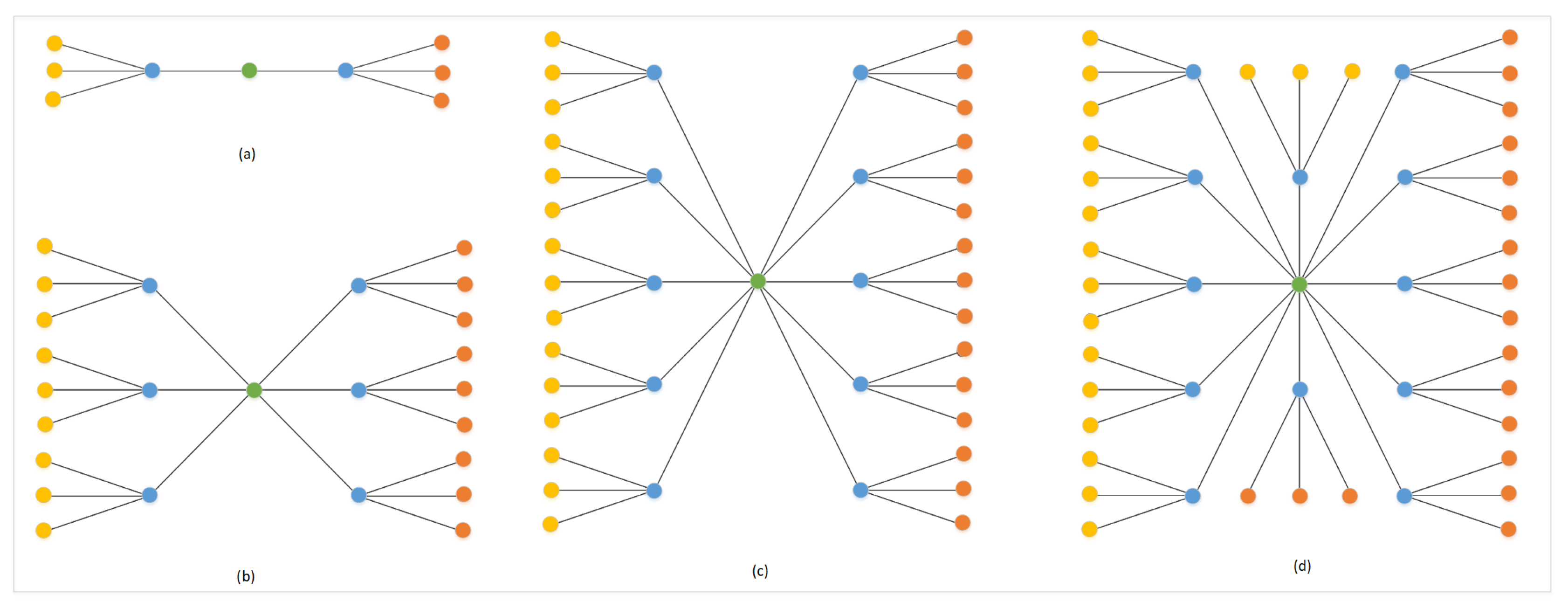
The network topologies employed in the simulations are presented in Figure 3. The orange-colored nodes show the WAPs deployed in an ultra-dense network to give Internet access to the end users. The WAPs are connected to the high-power cloud devices (red color) via a high-powered edge device (green color). The edge device is connected at a one-hop distance from the end-users and the cloud devices. It is to be noted that cloud devices are always located at multiple hops from the edge devices. However, for the sake of simplicity, we placed cloud devices at a one-hop distance from the edge device in our simulations and left the multihop statistical network analysis for future work.
We varied the number of WAPs and cloud devices and limited the edge device to one to create a bottleneck situation. These WAPs generated a large number of interest packets at a high frequency, i.e., 1000 interest packets per second. We chose to set the interest rate at a higher frequency to mimic massive traffic behavior in crowded areas.
To analyze the performance of the network, we calculated the ISR at each WAP. The ISR in a network is the ratio of the total number of satisfied interests to the total number of transmitted interests [27] and can be calculated using Equation (1), which is defined as follows:
I S R = 1 m satisfied interest 1 n transmitted interest × 100
where m is the total number of satisfied interests and n is the total number of transmitted interests.
The simulation was divided into two phases, to analyze the behavior of ISR. A detailed discussion of these two phases is explained in the following subsection.

3.1.1. Phase 1: Predictors Selection

In the first phase of simulation, multiple essential parameters, such as the number of nodes (NN), number of interests (NI), pending interest table (PIT), router bandwidth (RB), router delay (RD), content store (CS) capacity, and cache replacement strategies, were considered. A total of 90 simulation rounds were executed to analyze the behavior of the ISR thoroughly based on the aforementioned parameters. At first, the impact of the PIT timer was examined while holding all other parameters at their optimal values. A total of 20 simulation rounds were executed for the PIT timer. After analyzing the behavior of the PIT timer, we observed that it did not have much impact on the ISR. The reasons for this were: (1) the WAPs were at a one-hop distance from the edge device; (2) the link delay was a minimum of 10 ms; and (3) the RB was 20 Mbps; therefore, these values were satisfactory for satisfying the maximum number of packets. Moreover, the link was wired from the WAPs to the edge device. A wired link with no path loss or fading issues results in a higher packet delivery ratio, and hence, the network achieved a higher ISR. The reasons mentioned above led us to exclude the PIT timer parameter from our statistical analysis. In addition to the PIT timer, CS capacity (with various CS sizes) and various cache replacement policies were analyzed. A total of 40 rounds of simulations were executed to examine the impact of different cache replacement strategies and the cache capacity on the ISR. From the simulation results, we concluded that these two parameters were well suited for latency or round-trip time measurement analysis, since caching data closer to the client reduces latency and round-trip time. Therefore, we also excluded these two parameters from our current analysis and left the latency and round-trip time measurement analysis for future work.
In the second phase, we simulated 256 rounds, which included NN, NI, RB, and RD. The simulation rounds were based on a four-way factorial design. An overview of the factorial design method along with the details of the network parameters and their variations are presented in the following section.

3.1.2. Phase 2: Dataset Generation

In the second phase, we simulated 256 rounds, which included NN, NI, RB, and RD. The simulation rounds were based on a four-way factorial design. An overview of the factorial design method along with details of the network parameters and their variations are presented in the following section.

3.2. Four-Way Factorial Design

In experimental studies, there may be multiple factors that significantly impact the outcome. For an experiment, a quantitative variable can be designed to be qualitative, taking only a few pre-designed values, which are called levels.
For example, in ultra-dense networks, the bandwidth of a wireless or wired link can be considered as a factor with levels such as 1 Mbps, 2 Mbps, 10 Mbps, etc. In a factorial design, two or more factors can be involved in a single experiment. The number of levels for each of the factors can be different. In general, if K factors are used to design an experiment and the k th factor has lk levels, then the size of the experiment is given by N as in Equation (2).
N = k = 1 K l k
For the generation of the dataset, a complete four-way factorial design was used [28], where the four factors were NI with values at [250, 500, 750, 1000], NN with values at [9, 25, 41, 49], RB with values at [1, 5, 10, 20], and RD with values at [10, 50, 100, 200], as shown in Table 1. Four levels of each factor were used to reveal the non-linearity of the data. Including all the combinations of factors in the model, the linear model was as follows:
y i j k n q = μ + α i N I + α j N N + α k R B + α n R D + α i j N I × N N + α i k N I × R B + α i n N I × R D + α j k N N × R B + α j n N N × R D + α k n R B × R D + α i j k N I × N N × R B + α i j n N I × N N × R D α i k n N I × R B × R D + α j k n N N × R B × R D + α i j k n N I × N N × R B × R D + e i j k n q
In Equation (3), μ is the grand mean. α stands for fixed effects, with the superscripts denoting the factors and the subscripts denoting their levels. The interaction effect is indicated by × in the superscripts. Equation (3) tests the difference between levels of fixed effects since the fixed effects are considered as fixed categories.

4. Statistical Methods

This section briefly explains the statistical methods used in this paper.

4.1. Multiple Linear Regression

For the performance analysis of the ultra-dense network, this paper employs the MLR method [29]. MLR can often explain the relationship between a response variable and predictors by fitting a linear model to the observed experimental data. The response variable is often referred to as a dependent variable, whereas the predictor variables may be referred to as independent variables. The rationale for using MLR for the statistical analysis of an ultra-dense network is that (1) this reveals the impact magnitude of the predictor variables, such as NN, NI, RB, and RD on the response variable ISR; (2) how much the response variable changes according to the predictor variables; and (3) it predicts the future values of the response variable. For example, it may help to predict the values of ISR for different values of the factors not presented in Table 1. The linear regression model with n predictor variables x 1 , x 2 , ⋯, x n can be defined as follows:
y i = β 0 + β 1 x 1 i + β 2 x 2 i + + β n x n i + ϵ i for i = 1 , 2 , , n
where y i is a response variable (ISR), x 1 i i = 1 , 2 , , n are the predictor variables, and the ϵ i are random errors in the model. The coefficient β 0 is the y-intercept at Time 0. β 1 , 2 , , n are coefficients that measure the change in the response variable when x i ( 1 , 2 , , n ) changes by a unit. Equation (4) treats the difference between levels as a continuous; hence, it estimates the coefficients that can be interpreted as slopes.
In the analysis of variance (ANOVA) table for the MLR, the individual p-values were less than the significance level of 0.05, indicating that the corresponding predictor was significant. The magnitude and sign of the coefficient describe the size of the positive or negative relationship that exists between the predictor variables and the response variable. A positive sign of the coefficient estimate shows that as the value of the predictor variable increases, the mean value of the response variable also increases. A negative sign of the coefficient estimate indicates that as the predictor variable increases, the mean of response variable decreases. Moreover, the coefficient estimates can also be used to analyze the effect of an individual predictor on the response variable by holding all other predictors constant. The standard error measures the accuracy of the coefficient estimates. A small standard error shows that the observations are close to the fitted line.
As shown in Equation (4), there could be multiple predictor variables in the model that explain the response variable. Some of these are insignificant, while others are not. The existence of insignificant or irrelevant predictors in the model decreases the precision and conceals the genuine predictor. Most regression analyses repeatedly carry out the process of removing those irrelevant predictors from the model until only significant predictors are left in the model. Any variable with a p-value less than the significance level 0.05 is significant.

4.2. Akaike Information Criterion

The AIC measures the relative quality of statistical models when models are compared. The AIC is defined based on the maximum likelihood estimators of the parameters, as follows:
A I C = M L L + 2 k
where M L L is the maximum log-likelihood function and K is the number of parameters to be estimated in the model.
Among a set of candidate models for the given data, the model with the smallest AIC is the best. The AIC rewards goodness-of-fit assessed by MLL, but imposes a penalty on the number of parameters in the models. The penalty in the AIC discourages over-fitting caused by an excessive number of parameters in the model, which sometimes improves the goodness-of-fit.

4.3. Main and Interaction Effects

The main effect [30] is the average effect of a single predictor on the response variable across all other predictors involved in the experiment. In this study, we analyzed an individual predictor out of all the independent variables NN, NI, RB, and RD in order to find out whether it had a significant overall impact on the response variable ISR.
In more complex studies, however, it is possible that some predictors will interact with each other, and the effect of one predictor depends on the others. For example, if the means at the levels of NN significantly depend on the RD levels, then there is an interaction between NN and RD. The change of one predictor NN does not influence the effect of the other predictor RD on the response variable ISR if there is no interaction effect between the two predictors. Based on the conjecture derived from the mean plots of the main effects, interaction plots, and the multiple comparison test, candidate main effects and interaction effects were included as starting variables in the further regression analysis.

4.4. Multiple Comparison Test

As the start of analysis on which the predictor had a substantial impact on a response variable ISR, a multiple comparison test was conducted to find whether the notable difference in mean ISR arose according to the levels of each predictor. The multiple comparison test [31] involves N k pairwise comparison tests, each of which estimates and compares the two paired means.
Tukey’s honestly significant difference (HSD) [32] test is one of the most popular multiple comparison tests that detect the difference among the levels of a given factor. For each pair, Tukey’s HSD test is defined by:
H S D = M i M j M S w n h
where M i M j is the difference between the pair of means, M S w is within the mean sum of squares, and n h is the group or treatment number.

5. Results

5.1. Main Effect

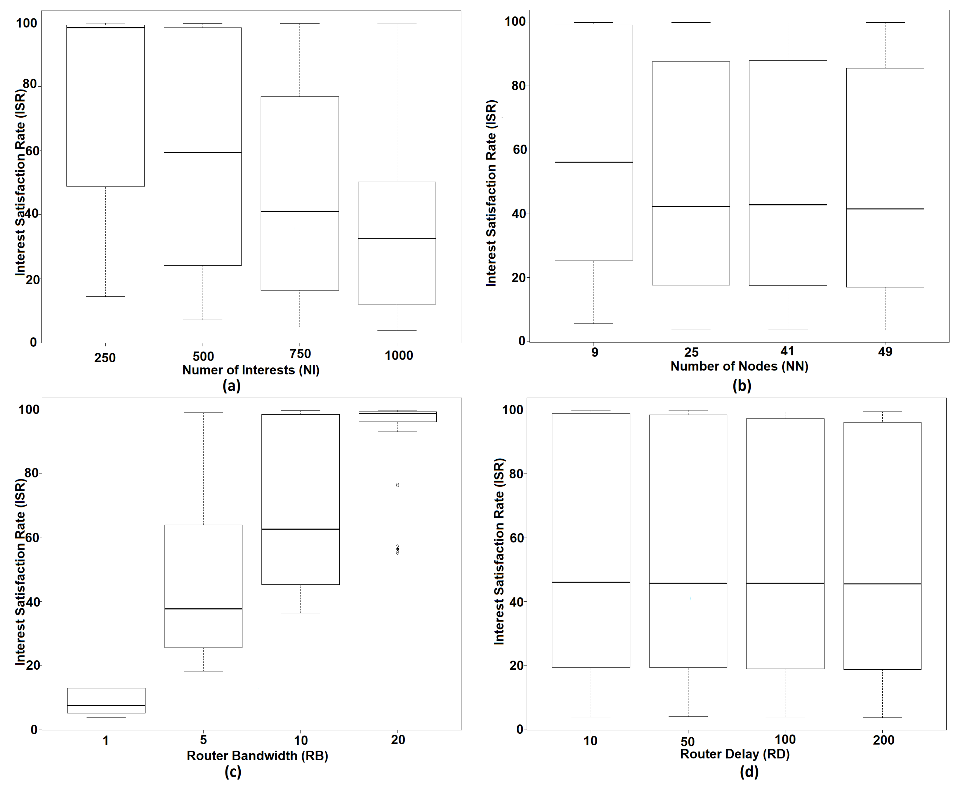
We first evaluated the main effects of predictors and how they influenced the response variable. Figure 4a shows the mean effect at the levels of NI. The mean ISR is approximately 98% when NI is 250, and it decreases to 59% when NI is increased to 500. The mean ISR is 40% and 33% at NI equal to 750 and 1000, respectively. From Figure 4a, NI shows a negative effect on the ISR.
Figure 4b shows the mean effect at the levels of NN. The mean ISR was approximately 58% when NN was nine, and it decreased to 43% when NN was 25, 41, and 49. In Figure 4b, the NN showed a non-linear effect on the ISR. By grouping NN into two categories NN less than 10 and NN greater than 10, NN showed a negative effect on the ISR.
Figure 4c shows the mean effect at the levels of RB. The mean ISR was approximately 9% when RB was 1 Mbps, and it increased to 38% when NI was 5 Mbps. The mean ISR was 65% and 99% at RB equal to 10 Mbps and 20 Mbps, respectively. In Figure 4c, RB shows a positive effect on the ISR. The ranges of the four boxplots were quite different compared to the other predictors. Although the ISR appeared to increase according to a line in view of their medians, it also seemed to increase according to a log(RB) in view of their ranges. There were some outliers at RB = 20, which is extremely small compared to other observations.
Figure 4d shows the mean effect at the levels of RD. The mean ISR was approximately 45% at each level of RD, which indicated the absence of a main effect. In Figure 4d, RD shows no effect on the ISR.
In addition to mean plots of the four main effects, we performed Tukey’s HSD test (Table 2). For NI, all pairs 250–500, 250–750, 250–1000, 500–750, 500–1000, and 750–1000 were significantly different from each other. For NN, Group 1, which included nine nodes, was significantly different from the group, which included 25, 41, and 49 nodes. For RB, all pairs 1–5, 1–10, 1–20, 5–10, 5–20, and 10–20 were significantly different. For RD, none of the pairs were significantly different. The estimates in Table 2 show the size of the difference in ISR means for the pairs.

5.2. Interaction Effects

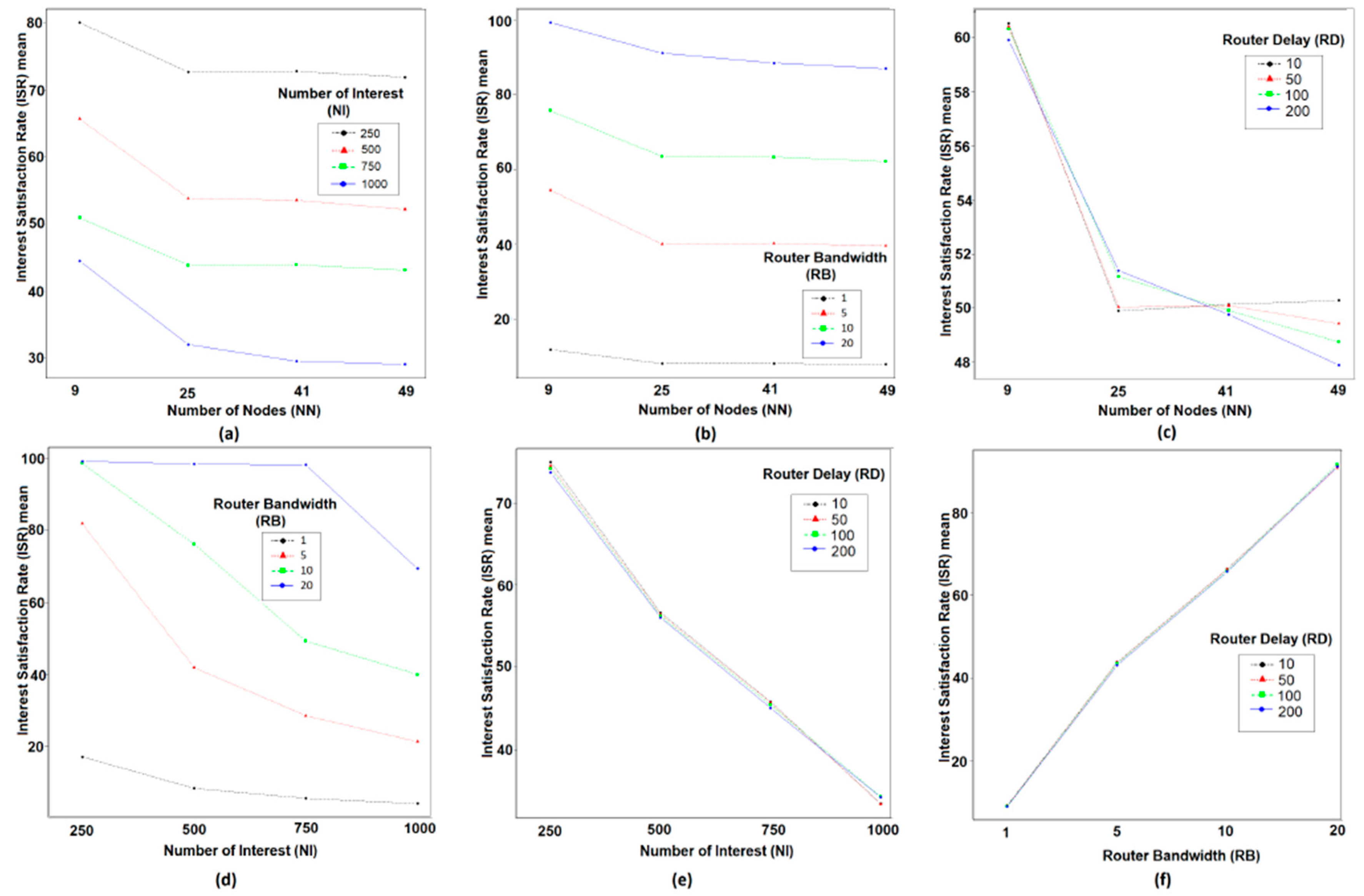
Figure 5 illustrates all six two-way interactions of the four predictor variables. In Figure 5a, the four parallel lines show similar trends. Since they did not intersect, there appeared to be no interaction effect between NN and NI. Similarly, in Figure 5b, the four almost parallel lines showed similar trends. Since they did not intersect, there appeared to be no interaction effect between NN and RB. The lines in Figure 5c intersected when NN was set at 12 and 38, which indicated the possible presence of an interaction effect between NN and RD. In Figure 5d, the lines were not parallel, even though they were not within the given range, which indicated the possible presence of an interaction effect. In Figure 5e,f, the lines almost overlapped, which indicated no interaction at all.

5.3. Model Selection

Starting from the initial model, including the candidate predictors with four levels and their interactions chosen from the mean plots, interaction plots, and multiple comparison tests, we selected the best model based on the AIC. The step AIC in R [33] was used to process a stepwise selection of variables, where the model with the smallest AIC was selected from among all possible models for given predictors. Once the best model was selected based on the AIC, we defined new variables using a transformation for better fit, and the linear models will again be fitted based on the newly-defined predictors. For each model, the ANOVA tables were presented with estimates of factors and their standard errors, p-values, and goodness-of-fit statistics, including F-statistics, R 2 , adjusted R 2 , and the AIC.

5.3.1. Initial Model

In the following initial model (Equation (7)), all predictors (NN, NI, RB, and RD) and all of their two-way interactions were included.
I S R = β 0 + β N N N N + β N I N I + β R B R B + β R D R D + β N N × N I N N × N I + β N N × R B N N × R B + β N N × R D N N × R D + β N I × R B N I × R B + β N I × R D N I × R D + β R B × R D R B × R D + ϵ
The coefficient estimates and their corresponding p-values are presented in Table 3. The coefficients in the MLR were the intercept and slopes. The intercept was the grand mean of the ISR, which became the baseline of all observations. The F-statistic for the model accuracy was significant (p < 2.2 × 10 16 ), implying that there was at least one predictor that had a significant effect on the ISR.
Model 1 included all candidate predictors with four levels and their interactions chosen from mean plots, interaction plots, and multiple comparison tests. In Model 1, the only significant predictors were NI and RB; this did not agree with the result from the previous mean plots and multiple comparison tests. An NN of nine is supposed to have a significantly different effect on the ISR compared to an NN of 25, 41, and 49. This phenomenon occurs when nuisance predictors with multicollinearity are included in the model. Therefore, stepAIC was employed to select significant predictors and remove unnecessary ones from the model.

5.3.2. Step AIC

The stepAIC function in R selects the model with the smallest AIC from among all possible linear models with provided predictors. Table 4 presents the coefficient estimates of the final selection of predictors and their corresponding p-values. The AIC of the model selected by stepAIC (AIC = 1369.39) was smaller than that of Model 1 presented in Table 3 (AIC = 1381.59).
Model 2 (Equation (8)) includes only three predictors (NN, NI, and RB), which have a significant impact on the ISR.
I S R = β 0 + β N N N N + β N I N I + β R B R B + ϵ
However, NN had less significant impact than RB and NI. Considering Figure 4b and Tukey’s HSD test in Table 2, NN was redefined into one of two categories: (1) NN less than 10 and (2) NN greater than 10.

5.3.3. Model with Categorical NN

Let us categorize NN to define N N F , which is a dummy variable.
N N F = 0   for   N N < 10   and   N N F = 1   for   N N 10
Model 3 (Equation (9)) was fitted with NI, N N F , and RB. Moreover, Model 3 had the smallest AIC value among the previously-presented Models 1 and 2.
I S R = β 0 + β N N F N N F + β N I N I + β R B R B + ϵ
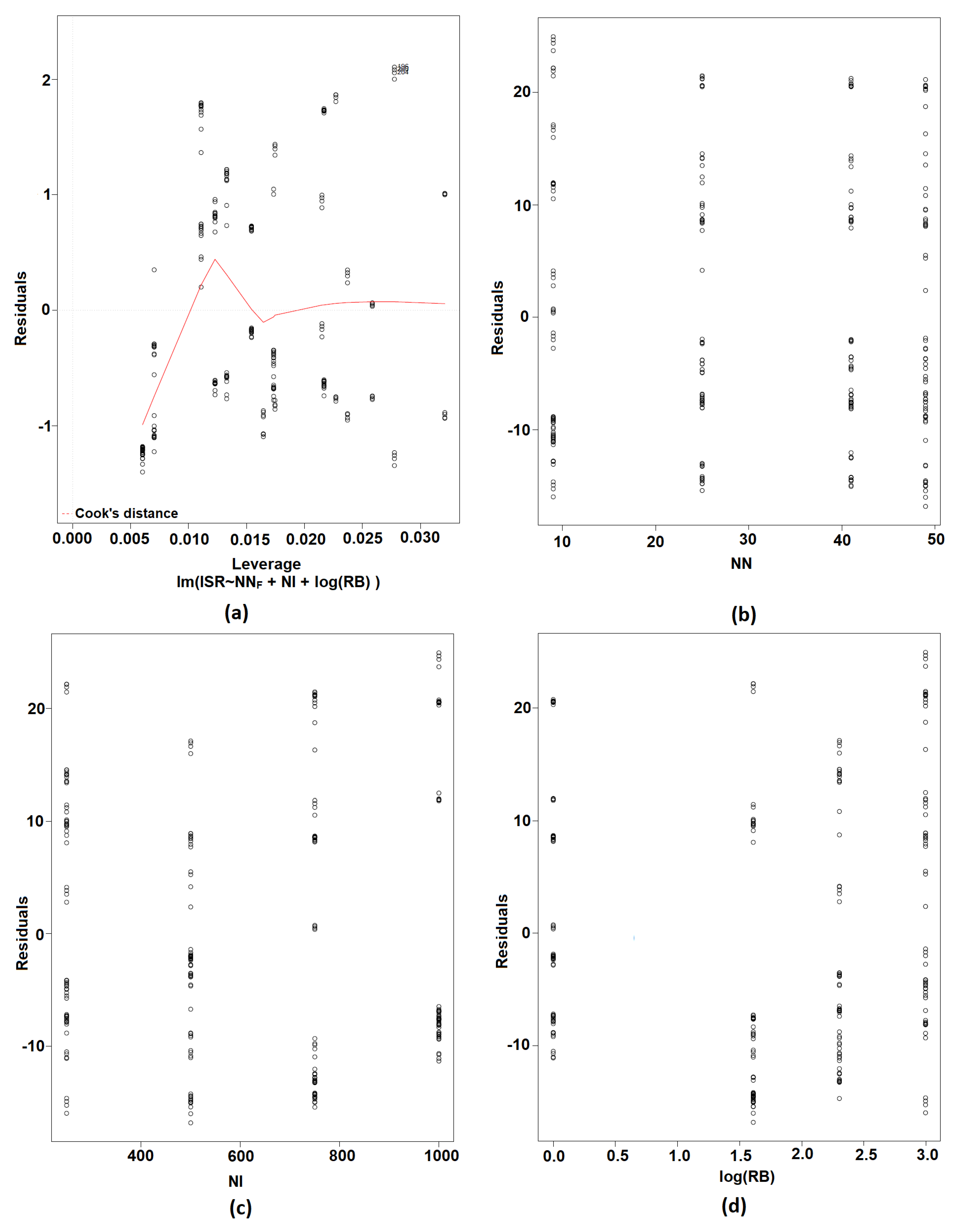
The β N N F = 10 . 402083 for Model 3, which was less than zero. This indicated that NN < 10 had a significantly greater impact on the ISR than NN > 10. Although all of the predictors ( N N F , NI, and RB) were significant, the residual plots of RB showed a quadratic curve.

5.3.4. Final Model

Due to the curve in the residual plot of RB of Model 3, R B 2 was used in an initial attempt to fit the model. The model with R B 2 , however, returned a concave downward quadratic function, which did not agree with the fact that an increase in RB would increase the ISR. Therefore, the final model (Equation (10)) was instead fitted based on log(RB).
I S R = 46 . 67 + ( 10.40 ) N N F + ( 0.05 ) N I + ( 27.05 ) l o g ( R B )
Table 5 presents the coefficient estimates of the final model and their corresponding p-values. The AIC of the final model selected by stepAIC (AIC = 1276.49) was much smaller than those of the previous models.
Moreover, the accuracy of the models was also validated by employing residual graphs. In Figure 6, the residual graph shows the residual on the vertical axis and the predictor variable on the horizontal axis. The residual plots for the final model showed adequate goodness of fit. There were no trends in the residual plots.

6. Discussion

In the following, we include a discussion of some aspects that detail our findings in the statistical analysis of the named data ultra-dense network.
First, take a look at individual predictors one by one. It is evident from the results that when NI was at 250, the network achieved a higher mean ISR of approximately 98%. The mean ISR decreased when NI was set higher than 250, and until NI = 500, the network achieved the maximum ISR value of 60%. If the aim was to get a higher ISR in the network, then the NI value should be equal to or less than around 250. In other words, if there were multiple users in the stadium, then a maximum of approximately 250 requests per second should be allowed from individual users towards the edge node. By doing this, the network may achieve a higher packet delivery ratio or ISR. However, if the requirement was exceeded and thus the network needed to allow more than 250 requests per second, then requests must be forwarded towards other edge nodes to ease the burden on the single edge node.
The NN had a significant impact on the ISR. Dividing the NN into two groups NN less than 10 and NN greater than 10 had a significantly different impact on the ISR. The mean effect on the ISR was relatively constant when the number of nodes was between 25 and 49. The network attained a maximum (third quartile) of 85% ISR when the NN was set at 25–49. However, when the number of nodes was less than 10, the network achieved the maximum (third quartile) 99% ISR. For the network goal to achieve at least 80% ISR, there should be approximately 25 WAPs, which are optimal for a single edge node. However, in this case, each WAP or IoT device should not forward more than 250 interests per second. Since 250 requests per second are in fact a very high number of requests from the 25 WAPs, including the NN and NI in the network analysis can provide a better prediction with a higher interest satisfaction rate.
RB had a very significant impact on ISR. When the RB was set at 1 Mbps, the network achieved a small degree of the ISR. However, when the RB was set at 20 Mbps, the network achieved higher ISR. When the RB was in the middle bandwidths of 5 and 10 Mbps, the range of the ISR was wide and shifted upward. Because of this phenomenon, the log(RB) better fit than the RB to predict the ISR. For the RB to be at 20 Mbps, the mean ISR and maximum ISR were raised to approximately 99%, which was optimal for the maximum ISR. In other words, the bandwidth from the WAP to the edge device should be at least 20 Mbps if the goal of the network was to achieve the highest packet delivery ratio with 250 requests per second from a maximum of 25 nodes.
Although the two interaction plots appeared to reveal slight interactions between NN and RD and NI and RB, they turned out to be insignificant. The nonexistence of interaction effects between selected predictors is a revealing discovery since the predictors can be considered independent in the design of the ultra-dense network. Based on the model that includes NI, NN with two categories of less than 10 or greater than 10 and log(RB), the behavior of ISR can be further predicted for the predictor values that are not used in the dataset or simulations.
All three factors, NN, NI, and RB, are essential and must be included in the design considerations of ultra-dense networks. The statistical analysis results presented in our paper had the potential to address the four essential design requirements (multimedia support, real-time and reliable connection, edge computing, and bottleneck mitigation) of ultra-dense networks by choosing an appropriate level of each predictor.

7. Conclusions

In this paper, we presented a statistical performance analysis of an ultra-dense network by considering NDN as a network layer protocol. The position of this paper was threefold. First, a four-way factorial design method was presented, which was applied to generate the dataset, including various network parameters, in the ndnSIM simulator. Second, we evaluated these network parameters based on mean plots and interaction plots and used multiple comparison tests to analyze how the main effects and interaction effects influenced the ISR. Third, we selected an adequate MLR model to fit the ISR based on both the AIC and the coefficient of determination R 2 . Results showed that the response variable ISR was strongly dependent on NN, NI, and RB. Any variation in these variables may result in a significant change in the ISR. An NN of less than 10 had a more significant effect on the ISR than an NN greater than 10. The NI had a negative effect on the ISR. Log(RB) worked better than RB itself to fit the ISR by reducing the significant amount of AIC. In the final model, R 2 was 88.95%, which was very high and indicated that the model explained almost all of the variability of the response data around its mean.
The current study considered the communication between WAPs and edge devices, as deployed in a crowded area, to analyze the behavior of ISR. In future work, we aim to extend the statistical performance analysis to wireless communications between end-users and WAPs to develop a suitable experimental design that could be helpful when designing a wireless network infrastructure for crowded areas.

Author Contributions

Conceptualization, M.A.U.R. and K.C.; methodology, M.A.U.R., K.C., and B.S.K.; validation, M.A.U.R., R.U., D.K., K.C., and B.S.K.; formal analysis, M.A.U.R., D.K., and R.U.; investigation, B.S.K., K.C., M.A.U.R., and R.U.; resources, B.S.K.; writing, original draft preparation, M.A.U.R.; writing, review and editing, M.A.U.R., R.U., K.C., and B.S.K.; supervision, K.C. and B.S.K.; funding acquisition, B.S.K.

Funding

This research was supported by the National Research Foundation of Korea (NRF) through the Korean Government (2018R1A2B6002399).

Conflicts of Interest

The authors declare no conflict of interest.

References

  1. Ullah, R.; Ahmed, S.H.; Kim, B. Information-Centric Networking with Edge Computing for IoT: Research Challenges and Future Directions. IEEE Access 2018, 6, 73465–73488. [Google Scholar] [CrossRef]
  2. Busari, S.A.; Huq, K.M.S.; Mumtaz, S.; Dai, L.; Rodriguez, J. Millimeter-Wave Massive MIMO Communication for Future Wireless Systems: A Survey. IEEE Commun. Surv. Tutor. 2018, 20, 836–869. [Google Scholar] [CrossRef]
  3. Wang, X.; Kong, L.; Kong, F.; Qiu, F.; Xia, M.; Arnon, S.; Chen, G. Millimeter Wave Communication: A Comprehensive Survey. IEEE Commun. Surv. Tutor. 2018, 20, 1616–1653. [Google Scholar] [CrossRef]
  4. Ullah, R.; Faheem, Y.; Kim, B. Energy and Congestion-Aware Routing Metric for Smart Grid AMI Networks in Smart City. IEEE Access 2017, 5, 13799–13810. [Google Scholar] [CrossRef]
  5. Parane, K.A.; Patil, N.C.; Poojara, S.R.; Kamble, T.S. Cloud based Intelligent Healthcare Monitoring System. In Proceedings of the 2014 International Conference on Issues and Challenges in Intelligent Computing Techniques (ICICT), Ghaziabad, India, 7–8 February 2014; pp. 697–701. [Google Scholar] [CrossRef]
  6. Rajasekhar, M.V.; Jaswal, A.K. Autonomous vehicles: The future of automobiles. In Proceedings of the 2015 IEEE International Transportation Electrification Conference (ITEC), Chennai, India, 27–29 August 2015; pp. 1–6. [Google Scholar] [CrossRef]
  7. Sisinni, E.; Saifullah, A.; Han, S.; Jennehag, U.; Gidlund, M. Industrial Internet of Things: Challenges, Opportunities, and Directions. IEEE Trans. Ind. Inform. 2018, 14, 4724–4734. [Google Scholar] [CrossRef]
  8. Cristina, G.N.; Gheorghita, G.V.; Ioan, U. Gradual Development of an IoT Architecture for Real-World Things. In Proceedings of the 2015 IEEE European Modelling Symposium (EMS), Madrid, Spain, 6–8 October 2015; pp. 344–349. [Google Scholar] [CrossRef]
  9. Cisco Visual Networking Index Predicts Near-Tripling of IP Traffic by 2020. Cisco, San Jose, CA, USA. 2017. Available online: https://newsroom.cisco.com/press-release-content?type=press-release&articleId=1771211 (accessed on 24 March 2019).
  10. Shang, W.; Yu, Y.; Droms, R.; Zhang, L. Challenges in IoT Networking via TCP/IP Architecture. NDN Project, Tech. Rep. NDN0038, February 2016. Available online: https://named-data.net/wp-content/uploads/2016/02/ndn-0038-1-challenges-iot.pdf (accessed on 13 March 2019).
  11. Jacobson, V.; Smetters, D.K.; Thornton, J.D.; Plass, M.F.; Briggs, N.H.; Braynard, R.L. Networking named content. In Proceedings of the 5th International Conference on Emerging Networking Experiments and Technologies (CoNEXT ’09), Rome, Italy, 1–4 December 2009; ACM: New York, NY, USA, 2009; pp. 1–12. [Google Scholar]
  12. Ahlgren, B.; Dannewitz, C.; Imbrenda, C.; Kutscher, D.; Ohlman, B. A survey of information-centric networking. IEEE Commun. Mag. 2012, 50, 26–36. [Google Scholar] [CrossRef]
  13. Afanasyev, A.; Shi, J.; Zhang, B.; Zhang, L.; Moiseenko, I.; Yu, Y.; Shang, W.; Li, Y.; Mastorakis, S.; Huang, Y.; et al. NFD Developer’s Guide; Technical Report, NDN-0021, NDN; University of California: Los Angeles, CA, USA, 2018. [Google Scholar]
  14. Ullah, R.; Rehman, M.A.U.; Kim, B. Design and Implementation of an Open Source Framework and Prototype For Named Data Networking-Based Edge Cloud Computing System. IEEE Access 2019, 7, 57741–57759. [Google Scholar] [CrossRef]
  15. Ahmed, S.H.; Bouk, S.H.; Yaqub, M.A.; Kim, D.; Song, H.; Lloret, J. CODIE: Controlled Data and Interest Evaluation in Vehicular Named Data Networks. IEEE Trans. Veh. Technol. 2016, 65, 3954–3963. [Google Scholar] [CrossRef]
  16. Ullah, R.; Rehman, M.A.U.; Kim, B.S. Hierarchical Name-Based Mechanism for Push-Data Broadcast Control in Information-Centric Multihop Wireless Networks. Sensors 2019, 19, 3034. [Google Scholar] [CrossRef]
  17. Din, I.U.; Hassan, S.; Khan, M.K.; Guizani, M.; Ghazali, O.; Habbal, A. Caching in Information-Centric Networking: Strategies, Challenges, and Future Research Directions. IEEE Commun. Surv. Tutor. 2018, 20, 1443–1474. [Google Scholar] [CrossRef]
  18. Osseiran, A.; Boccardi, F.; Braun, V.; Kusume, K.; Marsch, P.; Maternia, M.; Queseth, O.; Schellmann, M.; Schotten, H.; Taoka, H.; et al. Scenarios for 5G mobile and wireless communications: The vision of the METIS project. IEEE Commun. Mag. 2014, 52, 26–35. [Google Scholar] [CrossRef]
  19. Sakamoto, Y.; Ishiguro, M.; Kitagawa, G. Akaike Information Criterion Statistics; KTK Scientific Publishers: Tokyo, Japan; D. Reidel Publishing: Dodrecht, The Netherlands, 1986. [Google Scholar]
  20. How to Design Better Wireless Networks for Stadiums. Case Study, September 2015. Available online: https://www.cei-das.com/wp-content/uploads/iBwave-Case-Study-Stadiums.pdf (accessed on 8 March 2019).
  21. Guo, H.; Liu, J.; Zhang, J. Computation Offloading for Multi-Access Mobile Edge Computing in Ultra-Dense Networks. IEEE Commun. Mag. 2018, 56, 14–19. [Google Scholar] [CrossRef]
  22. Kamel, M.; Hamouda, W.; Youssef, A. Ultra-dense networks: A survey. IEEE Commun. Surveys Tutor. 2016, 18, 2522–2545. [Google Scholar] [CrossRef]
  23. Shreesha, S.; Routray, S.K. Statistical modeling for communication networks. In Proceedings of the 2016 2nd International Conference on Applied and Theoretical Computing and Communication Technology (iCATccT), Bangalore, India, 21–23 July 2016; pp. 831–834. [Google Scholar] [CrossRef]
  24. Routray, S.K. Statistical Analysis and Modeling of Optical Transport Networks. Ph.D. Thesis, University of Aveiro, Aveiro, Portugal, 2015. [Google Scholar]
  25. Korotky, S.K. Network global expectation model: A statistical formalism for quickly quantifying network needs and costs. IEEE/OSA J. Light. Technol. 2004, 22, 703–722. [Google Scholar] [CrossRef]
  26. Mastorakis, S.; Afanasyev, A.; Zhang, L. On the evolution of ndnSIM: An open-source simulator for NDN experimentation. ACM SIGCOMM Comput. Commun. Rev. 2017, 47, 19–33. [Google Scholar] [CrossRef]
  27. Arshad, S.; Shahzaad, B.; Azam, M.A.; Loo, J.; Ahmed, S.H.; Aslam, S. Hierarchical and Flat-Based Hybrid Naming Scheme in Content-Centric Networks of Things. IEEE Internet Things J. 2018, 5, 1070–1080. [Google Scholar] [CrossRef]
  28. Collins, L.M.; Dziak, J.J.; Li, R. Design of experiments with multiple independent variables: a resource management perspective on complete and reduced factorial designs. Psychol. Methods 2009, 14, 202–224. [Google Scholar] [CrossRef] [PubMed]
  29. Rice, J.A. Mathematical Statistics and Data Analysis, 3rd ed.; Cengage Learning: Boston, MA, USA, 2007. [Google Scholar]
  30. Weinberg, S.; Abramowitz, S. Statistics Using SPSS; Cambridge University Press: New York, NY, USA, 2008. [Google Scholar]
  31. McHugh, M.L. Multiple comparison analysis testing in ANOVA. Biochem. Med. 2011, 21, 203–209. [Google Scholar] [CrossRef]
  32. Tukey, J. Comparing Individual Means in the Analysis of Variance. Biometrics 1949, 5, 99–114. [Google Scholar] [CrossRef] [PubMed]
  33. CRAN: Manuals—The R Project for Statistical Computing. Available online: https://cran.r-project.org/manuals.html (accessed on 4 February 2019).
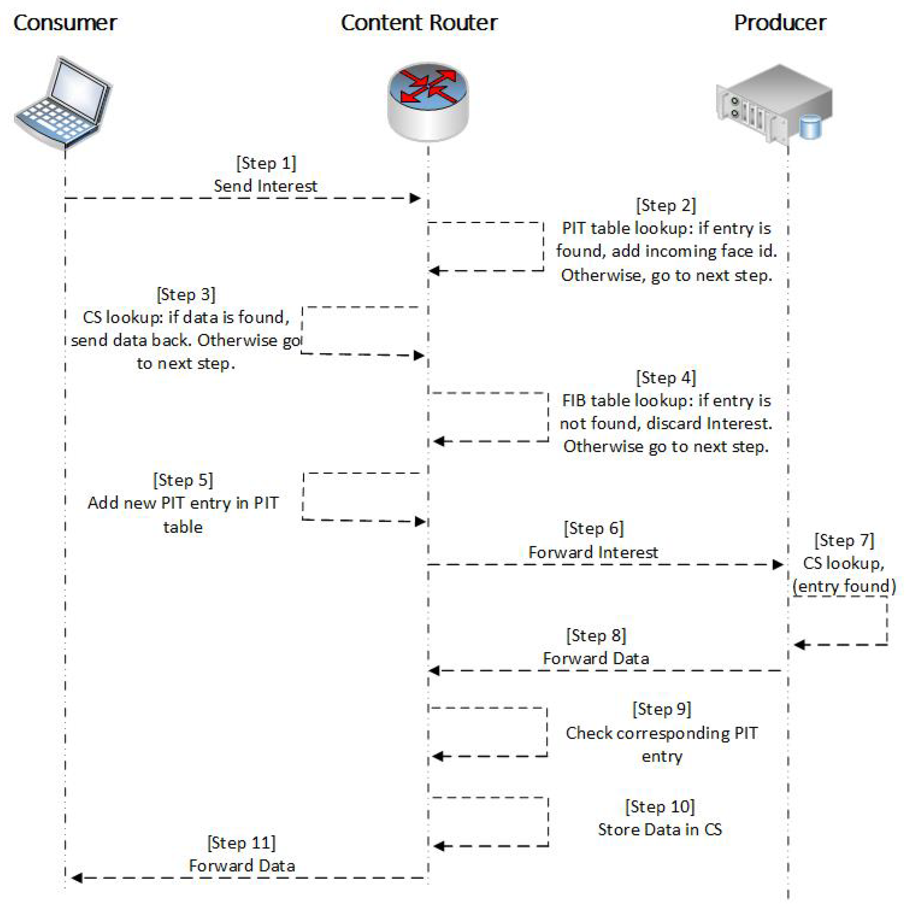
Figure 1. Named data networking (NDN) communication process. CS, content store; PIT, pending interest table; FIB, forwarding information base.
Applsci 09 03714 g001
Figure 2. Example of the communication scenario in a stadium.
Applsci 09 03714 g002
Figure 3. Network topologies: (a) 3 wireless access points, (b) 9 wireless access points, (c) 15 wireless access points, and (d) 21 wireless access points
Applsci 09 03714 g003
Figure 4. Mean plot for the main effect: (a) ISR as a function of the number of interest (NI), (b) ISR as a function of number of nodes (NN), (c) ISR as a function of router bandwidth (RB), and (d) ISR as a function of router delay (RD).
Applsci 09 03714 g004
Figure 5. Interaction effect plots: (a) NN vs. NI, (b) NN vs. RB, (c) NN vs. RD, (d) NI vs. RB, (e) NI vs. RD, and (f) RB vs. RD.
Applsci 09 03714 g005
Figure 6. Residuals plots: (a) residuals vs. leverage, (b) NN residuals, (c) NI residuals, and (d) log(RB) residuals.
Applsci 09 03714 g006
Table 1. Factors and the levels used in simulations.
FactorsLevels
Number of Interests (NI)250, 500, 750, 1000
Number of Nodes (NN)9, 25, 41, 49
Router Bandwidth in Mbps (RB)1, 5, 10, 20
Router Delay in ms (RD)10, 50, 100, 200
Table 2. Tukey’s honestly significant difference (HSD) test.
Levels250–500250–750250–1000500–750500–1000750–1000
NIp-values0008 × 10 7 01 × 10 7
estimates−18.01813−28.85063−40.51750−10.83250−22.49938−11.66688
Levels9–259–419–4925–4125–4941–49
NNp-values0.00001340.00000290.00000030.98816070.86837950.9706484
estimates−9.6742188−10.3223438−11.2096875−0.6481250−1.5354687−0.8873437
Levels1–51–101–205–105–2010–20
RBp-values000000
estimates34.5985957.2187582.5120322.6201647.9134425.29328
Levels10–5010–10010–20050–10050–200100–200
RDp-values0.99952040.99976710.99524380.99999520.99925160.9987582
estimates−0.2200000−0.1728125−0.47531250.0471875−0.2553125−0.3025000
Table 3. Model 1 (ANOVA table).
EstimateStd. Errort-ValuePr (>| t |)
(Intercept)5.104 × 10 1 7.348 × 10 0 6.9463.36 × 10 11 ***
NN−6.763 × 10 2 1.796 × 10 1 −0.3770.707
NI−4.744 × 10 2 9.360 × 10 3 −5.0687.93 × 10 7 ***
RD−4.195 × 10 3 4.372 × 10 2 −0.0960.924
RB4.402 × 10 0 4.372 × 10 1 10.069<2 × 10 16 ***
NN:NI−1.716 × 10 4 2.117 × 10 4 −0.8100.419
NN:RD−2.298 × 10 4 8.328 × 10 4 −0.2760.783
NN:RB−7.338 × 10 3 8.328 × 10 3 −0.8810.379
NI:RD1.281 × 10 5 4.577 × 10 5 0.2800.780
NI:RB−1.501 × 10 4 4.577 × 10 4 −0.3280.743
RD:RB1.194 × 10 4 1.800 × 10 3 0.0660.947
Signif.codes: 0 “***”; 0.001 “**”; 0.01 “*”; 0.05 “.”; 0.1 “”” 1; residual standard error: 14.55 on 245 degrees of freedom; multiple R-squared: 0.8423, adjusted R-squared: 0.8359 F-statistic: 130.9 on 10 and 245 DF, p-value: <2.2 × 10 16 ; AIC: 1381.59.
Table 4. Model 2 (ANOVA table).
EstimateStd. Errort-ValuePr (>| t |)
(Intercept)56.8798403.07414518.503<2 × 10 16 ***
NN−0.2616020.058563−4.4671.2 × 10 5 ***
NI−0.0529540.003219−16.452<2 × 10 16 ***
RB4.0913700.12659932.317<2 × 10 16 ***
Signif. codes: 0 “***”; 0.001 “**”; 0.01 “*”; 0.05 “.”; 0.1 “”” 1; residual standard error: 14.39 on 252 degrees of freedom; multiple R-squared: 0.8412, adjusted R-squared: 0.8393; F-statistic: 445 on 3 and 252 DF, p-value: <2.2 × 10 16 ; AIC: 1369.39.
Table 5. Final Model (ANOVA table).
EstimateStd. Errort-valuePr (>| t |)
(Intercept)46.6774462.53529418.411<2 × 10 16 ***
factor(newNN)1−10.4020831.732878−6.0036.72 × 10 9 ***
NI−0.0529540.002685−19.725<2 × 10 16 ***
log(RB)27.0516920.67538740.054<2 × 10 16 ***
Signif. codes: 0 “***”; 0.001 “**”; 0.01 “*”; 0.05 “.”; 0.1 “”” 1; residual standard error: 12.01 on 252 degrees of freedom; multiple R-squared: 0.8895, adjusted R-squared: 0.8882; F-statistic: 676.5 on 3 and 252 DF, p-value: <2.2 × 10 16 ; AIC: 1276.49.