The Direct Integration Method with Virtual Initial Conditions on the Free and Forced Vibration of a System with Hysteretic Damping

Abstract

The energy dissipated in hysteretic damping is independent of cyclic frequency, which agrees with the experimental results of energy dispersion of many materials under cyclic loading. Despite these desirable properties, hysteretic damping suffers from a notable drawback; the direct integration solution of the equation of motion is divergent. In this paper, a virtual initial condition is proposed to address the instability of the solution. The new method develops virtual initial conditions associated to the real initial conditions, which make the direct integration solution eliminate the divergence term of the complementary solution and converge to the exact solution. The stability and accuracy of the proposed direct integration method are demonstrated to be effective in solving the divergence problem by the comparison of the numerical and theoretical solutions on the free and forced vibration of a system with hysteretic damping.

1. Introduction

Damping is the natural property of a vibration system, which dissipates vibration energy. The widely used models to represent damping in a system are the viscous model and the hysteretic model [1,2,3]. Viscous damping, whose force is proportional to the velocity, is the most popular model due to the mathematical convenience. However, it implies a dissipated energy per a vibration cycle depending on the frequency. Hysteretic damping, whose force is proportional to the displacement and in phase with the velocity, leads to a dissipated energy per cycle which is independent of the frequency [4,5]. Experiments on structural materials indicate that the energy dissipation is independent of the cyclic frequency [6,7,8]. In those cases, the hysteretic damping is more precise. However, there are some drawbacks in the solution of the equation of motion with hysteretic damping for both the frequency domain analysis and the direct integration method in the time domain, which hinders the wider application of hysteretic damping models.

The frequency domain approach solves the hysteretic damping system by using the Fourier transform for the equation of motion [9,10,11], but it has two main drawbacks [12,13]. (1) Part of transient response may be neglected which may underestimate the response at the initial time and (2) in theory, it is only applicable for the linear elastic system due to the application of the superposition principle, so it cannot be used to analyze the true nonlinear response. For the approximate solution of a nonlinear system, Idriss and Seed [14] proposed an equivalent linearization method, which was widely used in the nonlinear seismic response of soil site and soil-structure interaction [15,16,17,18].

In a time-domain analysis, the numerical method is widely used because of its high efficiency, and because it can analyze the nonlinear problems as well [19,20,21,22,23]. However, the result from the numerical method is divergent when the direct integration method is used to solve the hysteretic damping systems, even if the integration procedure is unconditionally stable [24]. To develop the hysteretic damping in the time domain, a common method is to transfer the hysteretic damping into the approximate viscous damping. Henwood [25] used the forcing frequency to replace the natural frequency. Thus, the hysteretic damping matrix can be transferred to a viscous damping matrix, which is independent of frequency. Chen [26] proposed an integral-differential equation (IDE) in the time domain for the free vibration of a single degree-of-freedom (SDOF) system by using viscous damping depending on the frequency to equivalent hysteretic damping. Zhou [27] combined the standard linear constitutive models to approximate the hysteretic damping constitutive model in the time domain, and then applied the time-step integral calculation to hysteretic damping model.

However, until now, the improvement in the direct integration of a hysteretic damping system is still very slow, and the divergence of the results of the direct integral method has not been solved. In theory, there are two kinds of unstable solutions for the direct integration method. One is caused by the instability of the numerical method, and the other is caused by the divergent solution of the equation itself. The instability of the direct integration method of the hysteretic damping model is caused by the latter one since the pair of eigenvalues of the SDOF hysteretic damping are complex numbers and opposite to each other. The complementary solution of the equation is a linear combination of the two eigenvalue exponential functions. Therefore, the eigenvalue with a positive real part will cause a divergent solution, which is contrary to the natural and physical phenomenon. In the theoretical solution, the divergent term can be arbitrarily omitted, but it is kept in the direct integration procedure. Recently, Sun [28] proposed a time-domain numerical method based on the interpolation of excitation, which is a semi-analytic direct integration method, by using the theoretical solution in each step.

Therefore, the key to the stability of the direct integration method of a hysteretic damping system is to eliminate the divergent term in the recursive process. In this paper, we propose to use virtual initial conditions to address the instability of the solution. The proposed method constructs virtual initial conditions by the real part of the displacement and velocity of the previous step, as well as the load condition, so that the direct integration solution converges to the exact solution. Except for the initial conditions, all the procedures of the proposed method are the same as the direct integration method for the governing equation of motion with viscous damping. Then, the stability and accuracy of the proposed direct integration method are demonstrated by the comparison of numerical and theoretical solutions on the free and forced vibration of the SDOF system with hysteretic damping.

2. Equation of Motion and the Direct Integration Method

The governing equation of motion of a single-degree-of-freedom (SDOF) system with hysteretic damping in forced vibration can be expressed as [29]

$$m\ddot{u}+(1+i\eta )ku=f\left(t\right),$$

(1)

where m and k are the mass and stiffness, respectively, η is the hysteretic damping factor, $i=\sqrt{-1}$, $\ddot{u}$ and $u$ are the acceleration and displacement of the SDOF, respectively, and $f(t)$ is the applied force. This equation is to be solved for the displacement, u(t), subjected to the initial conditions as

$$u(0)=u_0\mathrm{and}\dot{u}(0)=v_0,$$

(2)

where $u_0$ and $v_0$ are the displacement and velocity at the time t = 0.

For the direct integration method, let the time axis be divided into small intervals of equal length $\Delta t$, and let $t_n=n\Delta t$(n = 0, 1, 2, …. N) be the division times. The response of displacement, velocity, and acceleration at the discrete time instants $t_n$ are $u_n$, ${\dot{u}}_n$, and ${\ddot{u}}_n$. The applied force $f(t)$ at $t_n$ is $f_n$.

So far, several direct integration methods have been proposed to obtain the solution at time $t_{n+1}$ assuming that the solutions at times t_i (i = 0, 1, 2, …. n) are known. The Newmark method is used to investigate the stability of the solution of the hysteretic damped equation in the following illustration. In the Newmark method, the velocity and acceleration at time $t_{n+1}$ can be expressed as

$${\dot{u}}_{n+1}=\frac{\gamma }{\beta \Delta t}(u_{n+1}-u_n)+(1-\frac{\gamma }{\beta }){\dot{u}}_n+(1-\frac{\gamma }{2\beta }){\ddot{u}}_n\Delta t,$$

(3)

$${\ddot{u}}_{n+1}=\frac{1}{\beta \Delta t^2}(u_{n+1}-u_n)-\frac{1}{\beta \Delta t}{\dot{u}}_n-(\frac{1}{2\beta }-1){\ddot{u}}_n,$$

(4)

in which parameter $\gamma$ and $\beta$ are parameters that can be determined to obtain integration accuracy and stability. Substituting Equation (4) into Equation (1) gives:

$$\widehat{k}{u}_{n+1}={\widehat{f}}_{n+1},$$

(5)

where $\widehat{k}=(1+i\eta )k+\frac{1}{\beta \Delta t^2}m$ and ${\widehat{f}}_{n+1}=f_{n+1}+[\frac{1}{\beta \Delta t^2}{u}_n+\frac{1}{\beta \Delta t}{\dot{u}}_n+(\frac{1}{2\beta }-1){\ddot{u}}_n]m$. Solve the displacement, $u_{n+1}$, by Equation (5), then ${\dot{u}}_{n+1}$ may be determined from Equation (3) and the acceleration may be determined from the following expression deduced from Equation (1):

$${\ddot{u}}_{n+1}=\frac{f_{n+1}-(1+i\eta )k{u}_{n+1}}{m}.$$

(6)

It is well known that the Newmark method is unconditionally stable for $\gamma =\frac{1}{2}$ and $\beta =\frac{1}{4}$, which is called the average acceleration method. However, the results obtained by the average acceleration method will blow up for the hysteretic damping system, giving meaningless results. The reason is that the solution will converge to the divergent solution which is caused by the divergent member of the complementary solution of Equation (1) if the real-valued initial condition is used directly in the Newmark method. Therefore, in this paper, a modified initial condition in each time step is proposed to address the unstable phenomenon for direct integration.

3. The Formulation for the Virtual Initial Condition

3.1. The Virtual Initial Condition for Free Vibration

For a system in free vibration, the right-hand member of Equation (1) vanishes and gives

$$m\ddot{u}+(1+i\eta )ku=0.$$

(7)

The solution for the homogeneous equation is

$$u=C{e}^{\lambda t},$$

(8)

in which C is a constant and λ is eigenvalue. Substituting Equation (8) into Equation (7) leads to the algebraic equation:

$${\lambda }^{2}m+(1+i\eta )k=0.$$

(9)

The solutions of Equation (9) are

$${\lambda }_1=s,{\lambda }_2=-s,$$

(10)

$$s=\omega (a-ib),$$

(11)

where $\omega =\sqrt{k/m}$ is the undamped natural frequency, $a=\sqrt{\frac{-1+\sqrt{1+{\eta }^2}}{2}}$, $b=\sqrt{\frac{1+\sqrt{1+{\eta }^2}}{2}}$. The two eigenvalues are opposite numbers to each other. The general solution of Equation (7) is

$$u=C_1{e}^{st}+C_2{e}^{-st}.$$

(12)

The constant C₁ and C₂ in terms of the real-value initial conditions of Equation (2) may be determined from

$$C_1=\frac{s{u}_0+v_0}{2s},C_2=\frac{s{u}_0-v_0}{2s}.$$

(13)

Since the real part of s is a positive quantity, there would be a growing response along the time for the right-hand first member $C_1{e}^{st}$, which is a divergent term which is contrary to the physical rule and should be omitted. Therefore, by introducing $C_1=0$ the correct general solution can be expressed as

$$u=C{e}^{-st},$$

(14)

where C is a complex constant. Applying the initial condition of Equation (2) gives

$$C=u_0-i\frac{v_0+\omega a{u}_0}{\omega b}.$$

(15)

In the analytical solution, the divergent member can be omitted to obtain the exact solution of Equation (14). However, the direct integration solution converges to Equation (12). Therefore, it is crucial to make Equation (12) equal to Equation (14). In this paper, the virtual initial conditions $u_0^{v1}$ and $v_0^{v1}$ are proposed to achieve this goal. The total initial conditions are the sum of the real initial conditions and corresponding virtual initial conditions, that is

$$u_0^t=u_0^{}+u_0^{v1},v_0^t=v_0^{}+v_0^{v1}.$$

(16)

Substituting Equation (16) into Equation (13), and making Equation (12) equal to Equation (14), gives

$$\frac{s(u_0+u_0^{v1})+(v_0+v_0^{v1})}{2s}=0,$$

(17)

$$\frac{s(u_0+u_0^{v1})-(v_0+v_0^{v1})}{2s}=u_0-i\frac{v_0+\omega a{u}_0}{\omega b}.$$

(18)

Solving the two algebraic Equations (17) and (18) leads to

$$u_0^{v1}=-i\frac{v_0+\omega a{u}_0}{\omega b}.$$

(19)

$$v_0^{v1}=i[\frac{a}{b}(v_0+\omega a{u}_0)+\omega b{u}_0].$$

(20)

It can be seen that the virtual initial conditions are purely imaginary. The usual real initial conditions are

$$u_0^{}=\mathrm{Re}(u_0^t),v_0^{}=\mathrm{Re}(v_0^t).$$

(21)

It can be observed that the complete initial conditions are complex, but only the real parts can be observed and measured. The corresponding unobserved imaginary part should be the indivisible member of the initial condition. After introducing the virtual initial conditions, the general solution of Equation (7) is naturally exact, the real part of which is the observable solution and free decay.

3.2. The Virtual Initial Conditions for Harmonic Force

If f(t) is a harmonic force with forcing frequency θ, written as $A{e}^{i\theta t}$, the particular solution of Equation (1) is

$$u=X{e}^{i\theta t},$$

(22)

where $X=\frac{A}{-{\theta }^{2}m+(1+i\eta )k}$ The complementary solution is the free vibration response given by Equation (12). The complete solution is the sum of the complementary and particular solutions.

$$u=D{e}^{st}+E{e}^{-st}+X{e}^{i\theta t}.$$

(23)

The constants D and E are determined by the initial conditions. To illustrate conveniently, the virtual initial conditions associated with the real zero initial condition are deduced first. On applying the zero initial condition with $u(0)=0$ and $\dot{u}(0)=0$ to Equation (23), the constants D and E are deduced.

$$D=\frac{-s-i\theta }{2s}X,E=\frac{i\theta X-sX}{2s}.$$

(24)

Similar to the free vibration, the right-hand first term $D{e}^{st}$ is the divergent term and contrary to the physical rule, which should be omitted. The complete solution that is satisfied with physical meaning is

$$u=C_f{e}^{-st}+X{e}^{i\theta t}.$$

(25)

On making use of $u(0)=0$ and $\dot{u}(0)=0$ to Equation (25), the constant C_f is deduced as

$$C_f=-\mathrm{Re}(X)-i\frac{\theta \mathrm{Im}(X)-a\omega \mathrm{Re}(X)}{b\omega },$$

(26)

where $\mathrm{Re}(X)$ is the real part of X, and $\mathrm{Im}(X)$ is the imaginary part of X.

The direct integration solution converges to Equation (23), therefore, let Equation (23) be equal to Equation (25) by making use of the virtual initial condition $u_0^{v2}$ and $v_0^{v2}$. Subjected to initial displacement $u_0^{v2}$ and initial velocity $v_0^{v2}$, the constants D and E in Equation (23) are determined from

$$D+E+X=u_0^{v2},$$

(27)

$$sD-sE+i\theta X=v_0^{v2}.$$

(28)

Solving the two algebraic Equations (27) and (28) leads to

$$D=\frac{s{u}_0^{v2}+v_0^{v2}-sX-i\theta X}{2s},E=\frac{s{u}_0^{v2}-v_0^{v2}-sX+i\theta X}{2s}.$$

(29)

On making use of the identity between Equations (23) and (25), one obtains

$$\frac{s{u}_0^{v2}+v_0^{v2}-sX-i\theta X}{2s}=0,\frac{s{u}_0^{v2}-v_0^{v2}-sX+i\theta X}{2s}=C_f.$$

(30)

Then, it leads to

$$u_0^{v2}=C_f+X=i\frac{(b\omega -\theta )\mathrm{Im}(X)+a\omega \mathrm{Re}(X)}{b\omega },$$

(31)

$$v_0^{v2}=-s{C}_f+i\theta X=i\frac{a\theta \mathrm{Im}(X)+(b\theta -a^2\omega -b^2\omega )\mathrm{Re}(X)}{b}.$$

(32)

The virtual initial conditions $u_0^{v2}$ and $v_0^{v2}$ are also purely imaginary. The member $C_f{e}^{-st}$ in Equation (25) is free adjoint vibration which is independent of the real initial conditions but depends on the load. $u_0^{v2}$ and $v_0^{v2}$ are artificial load-dependent initial conditions which are developed to make the direct integration solution converges to the exact solution.

Equations (31) and (32) are deduced by the assumption that the system is initially at rest. For a system with non-zero initial conditions, the virtual initial conditions defined by Equations (31) and (32) should be augmented by the addition of the free vibrational solution defined by Equation (19) and (20). Then the total initial conditions of harmonic responses are

$$u_0^t=u_0^{}+u_0^{v1}+u_0^{v2},v_0^t=v_0^{}+v_0^{v1}+v_0^{v2}.$$

(33)

3.3. The Virtual Initial Conditions for Arbitrary Force

Assuming the SDOF system with hysteretic damping is subjected to real-valued force g₁(t), which varies arbitrarily with time, it is necessary to establish a dual force in the time domain analysis [30]. Then, the governing equation of motion can be written as

$$m\ddot{u}+(1+i\eta )ku=f(t)=g_1(t)+i{g}_2(t),$$

(34)

in which g₁(t) is the observable force, and g₂(t) is the corresponding dual force. By using discrete Fourier transforms (DFT), g₁(t) can be expanded to the sum of a series harmonic function, that is

$$g_1(t)=\frac{A_0}{2}+{\displaystyle \sum _{j=1}^{N/2-1}\left(A_j\cos {\theta }_{j}t+B_j\sin {\theta }_{j}t\right)}+\frac{A_{N/2}}{2}\cos {\theta }_{N/2}t,$$

(35)

where ${\theta }_j=\frac{2\pi j}{N\Delta t}$ (j = 0, 1, 2, …, N/2−1,N/2), $\Delta t$ is time intervals of discrete, Fourier coefficients $A_0$, $A_1$, $A_2$,…, $A_{N/2}$ and $B_1$, $B_2$,…, $B_{N/2-1}$ can be determined from

$$A_j=\frac{2}{N}{\displaystyle \sum _{l=0}^{N-1}{g}_1(t_l)}\cos ({\theta }_j{t}_l),j=0,1,2,\dots ,N/2-1,N/2,$$

(36)

$$B_j=\frac{2}{N}{\displaystyle \sum _{l=0}^{N-1}{g}_1(t_l)}\sin ({\theta }_j{t}_l),j=1,2,\dots ,N/2-1,$$

(37)

where $t_i=l\Delta t$ (l = 0, 1, 2, …, N−1) is the discrete value of t, g₁(t_l) is the discrete value of g₁(t).

Then dual loading g₂(t) can be expressed as

$$g_2(t)=\eta \frac{A_0}{2}+{\displaystyle \sum _{j=1}^{N/2-1}\left(A_j\sin {\theta }_{j}t-B_j\cos {\theta }_{j}t\right)}+\frac{A_{N/2}}{2}\sin {\theta }_{N/2}t.$$

(38)

So,

$$f(t)=\frac{A_0}{2}(1+i\eta )+{\displaystyle \sum _{j=1}^{N/2-1}\left(A_j-i{B}_j\right)e^{i{\theta }_{j}t}}+\frac{A_{N/2}}{2}{e}^{i{\theta }_{N/2}t}.$$

(39)

Equation (39) denotes that arbitrary force can be expressed as the sum of a series of harmonic forces, so the complete solution is the sum of a series of harmonic forces.

$$u={\displaystyle \sum _{j=0}^{N/2}\left(D_j{e}^{st}+E_j{e}^{-st}+X_j{e}^{i{\theta }_{j}t}\right)}.$$

(40)

The right-hand first term $D_j{e}^{st}$ is a divergent term and contrary to the physical rule and should be omitted, so the complete solution which is satisfied with physical meaning is

$$u={\displaystyle \sum _{j=0}^{N/2}\left(C_{fj}^{}{e}^{-st}+X_j{e}^{i{\theta }_{j}t}\right)},$$

(41)

where $X_0=\frac{A_0}{2k}$, $X_j=\frac{A_j-i{B}_j}{-{\theta }_j^{2}m+(1+i\eta )k}$(j = 1, 2, …, N/2−1), and $X_{N/2}=\frac{A_{N/2}}{2(-{\theta }_{N/2}^{2}m+(1+i\eta )k)}$.

On making use of $u(0)=0$ and $\dot{u}(0)=0$ to Equation (41), the constant C_fj is deduced.

$$C_{fj}=-\mathrm{Re}(X_j)-i\frac{{\theta }_j\mathrm{Im}(X_j)-a\omega \mathrm{Re}(X_j)}{b\omega }(j=0,1,2,\dots ,N/2).$$

(42)

Similar to the harmonic force, the virtual initial condition associated with each term can be determined from Equations (31) and (32) for the zero initial condition. Therefore, the virtual initial condition for arbitrary force can be expressed as

$$u_0^{v3}={\displaystyle \sum _{j=0}^{N/2}\left(C_{fj}+X_j\right)},$$

(43)

$$v_0^{v3}={\displaystyle \sum _{j=0}^{N/2}\left(-s{C}_{fj}+i{\theta }_j{X}_j\right)}.$$

(44)

Then the total initial conditions for a system with non-zero initial conditions are

$$u_0^t=u_0^{}+u_0^{v1}+u_0^{v3},v_0^t=v_0^{}+v_0^{v1}+v_0^{v3}.$$

(45)

Algorithm 1 summarizes the above-described procedure, which can be implanted into the computer. The procedure can also be used to calculate the free vibration and harmonic force with slight modification. Let $f_n=u_n^{v3}=v_n^{v3}=0$ for free vibration. The harmonic force is the particular example of the arbitrary force, which only keeps one term with the with forcing frequency θ to calculate $u_n^{v3}$ and $v_n^{v3}$. It is noted that step 2.4 is used to calculate the virtual initial condition for each time step n to eliminate the effect of the round-off and improve the accuracy. Then the stability is dependent on the β, γ.

Algorithm 1 Newmark method with the virtual initial condition for arbitrary force.

Step 1.0 Initial calculation

1.1 DFT for g1(t) to calculate coefficients Aj and Bj by Equations (36) and (37).

$1.2u_0^t=u_0^{}+u_0^{v1}+u_0^{v3},v_0^t=v_0^{}+v_0^{v1}+v_0^{v3}$

1.3 ${\ddot{u}}_0^t=\frac{f_0-(1+i\eta )k{u}_0^t}{m}$

1.4 $\mathrm{select}\Delta t,\mathsf{\beta },\mathsf{\gamma }$

1.5 $\widehat{k}=(1+i\eta )k+\frac{1}{\beta \Delta t^2}m$

Step 2.0 Calculations for each time step

2.1 ${\widehat{f}}_{n+1}=f_{n+1}+[\frac{1}{\beta \Delta t^2}{u}_n^t+\frac{1}{\beta \Delta t}{\dot{u}}_n^t+(\frac{1}{2\beta }-1){\ddot{u}}_n^t]m$

$2.2u_{n+1}={\widehat{f}}_{n+1}/\widehat{k}$

$2.3{\dot{u}}_{n+1}=\frac{\gamma }{\beta \Delta t}(u_{n+1}-u_n)+(1-\frac{\gamma }{\beta }){\dot{u}}_n+(1-\frac{\gamma }{2\beta }){\ddot{u}}_n\Delta t$

$2.4u_{n+1}^{v1}=-i\frac{\mathrm{Re}(v_{n+1})+\omega a\mathrm{Re}(u_{n+1})}{\omega b},v_{n+1}^{v1}=i[\frac{a}{b}(\mathrm{Re}(v_{n+1})+\omega a\mathrm{Re}(u_{n+1}))+\omega b\mathrm{Re}(u_{n+1})]$

$2.5u_{n+1}^t=\mathrm{Re}(u_{n+1})+u_{n+1}^{v1}+u_0^{v3},v_{n+1}^t=\mathrm{Re}(v_{n+1})+v_{n+1}^{v1}+v_0^{v3}$

$2.6{\ddot{u}}_{n+1}^t=\frac{f_{n+1}-(1+i\eta )k{u}_{n+1}^t}{m}$

Step 3.0 Repetition for the next time step. Replace n by n + 1 and implement step 2.1 to 2.6 for next time step.

4. Example Case Study

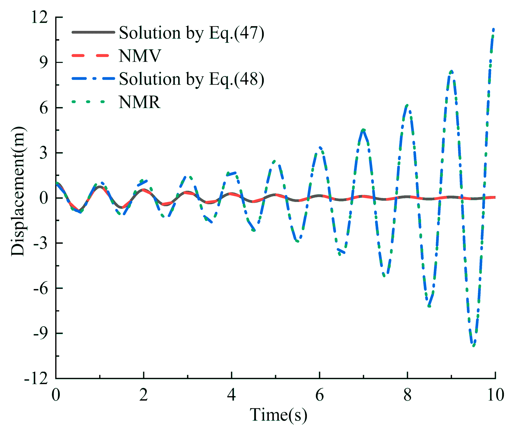
4.1. Free Vibration

This example case study analyzes an SDOF with free vibration, which has m = 1, k = 4π², and η = 0.1, considering the free vibration with the initial condition:

$$u_0=1\mathrm{and}{v}_0=0.$$

(46)

From Equation (14), the correct theoretical solution is

$$u=(1-0.05i)e^{(-0.314+6.291i)t}.$$

(47)

However, the wrong solution by Equation (12) with only the real initial conditions is

$$u=\frac{1}{2}{e}^{(0.314-6.291i)t}+\frac{1}{2}{e}^{(-0.314+6.291i)t}.$$

(48)

In this example, the problem was solved by the Newmark method with $\gamma =\frac{1}{2}$, $\beta =\frac{1}{4}$. The numerical results obtained using $\Delta t=0.01s$ are compared with the theoretical solution, as shown in Figure 1, in which NMV is numerical result obtained by algorithm 1, NMR is numerical result obtained by the Newmark method with real-valued initial conditions.

It can be seen from Figure 1 that if directly using the real initial conditions $u_0=1$ and $v_0=0$ by the Newmark method, the displacement blows up to give meaningless results which converge to the wrong solution of Equation (48). However, the displacement with initial conditions $u_0^t$ and $v_0^t$ by Equation (16) converges to the correct theoretical solution of Equation (47). Therefore, the Newmark method is stable, but the solution is unstable for the real initial conditions. After applying the proposed virtual initial condition, the divergent term is eliminated to make the solution stable.

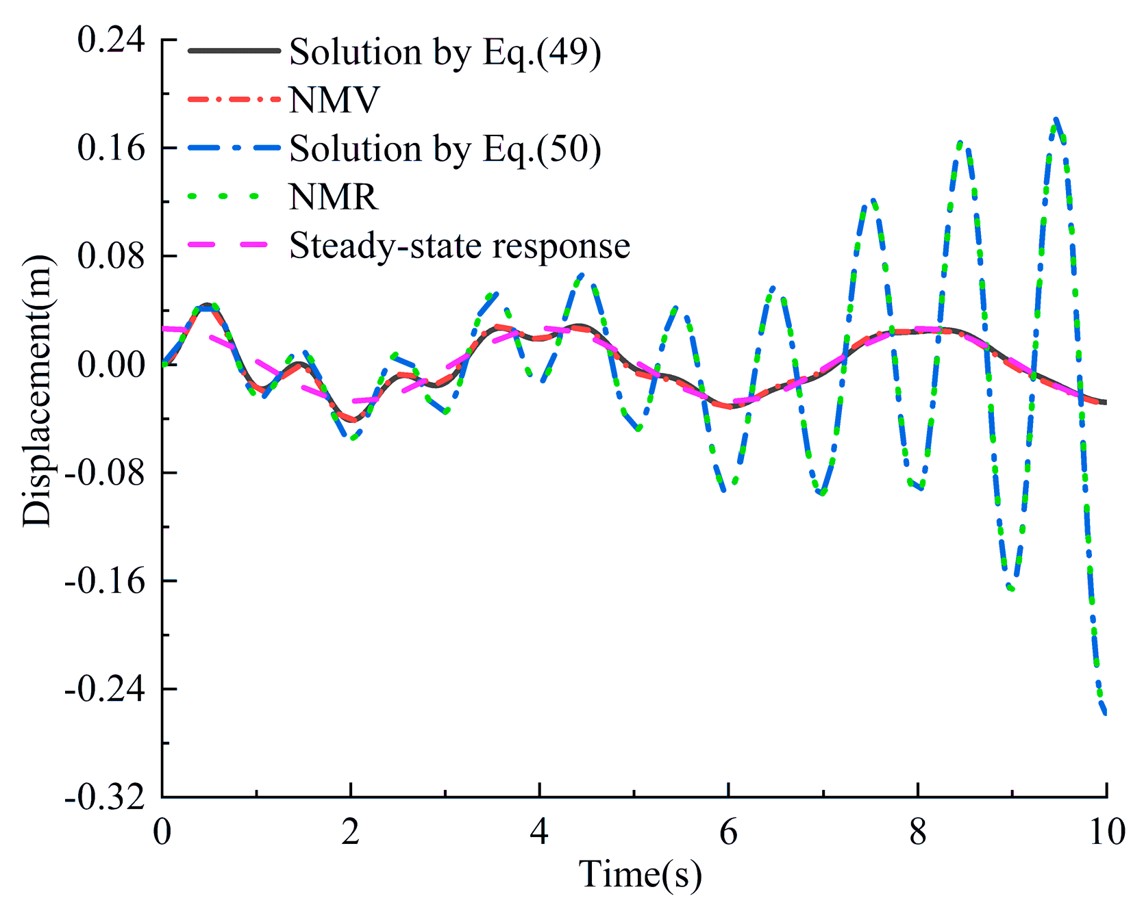
4.2. Harmonic Vibration

This example case study analyzed an SDOF subjected to harmonic force, $e^{i\theta t}$, with $\theta /\omega =0.25$, η = 0.1, m = 1, k = 4π², $u_0^{}=0$, $v_0^{}=0$. The correct theoretical solution by Equation (25) is expected to be

$$u=(-0.027+0.002i)e^{(-0.314+6.291i)t}+(0.027-0.0028i)e^{1.571it},$$

(49)

and the wrong solution by Equation (23) with only the real initial conditions is

$$u=(-0.01+0.0009i)e^{(0.314-6.291i)t}+(-0.0167+0.0019i)e^{(-0.314+6.291i)t}+(0.027-0.0028i)e^{1.571it}.$$

(50)

The solution of the steady-state response is

$$u=(0.027-0.0028i)e^{1.571it}.$$

(51)

The problem was also solved by the Newmark method with $\gamma =\frac{1}{2}$, $\beta =\frac{1}{4}$. The numerical results obtained using $\Delta t=0.01s$ are compared with the theoretical solution, as shown in Figure 2, as well as the solution of steady-state response. Obviously, the displacement blows up again for initial conditions $u_0=0$ and $v_0=0$, and it converges to the wrong solution of Equation (50). The result is stable and converges to the correct theoretical solution of Equation (49) for initial conditions $u_0^t$ and $v_0^t$. Therefore, for forced vibration, the unstable numerical solution is induced by the free adjoint vibration, which includes the divergent term. The virtual initial condition removed the divergent term so that the numerical solution is the same as the theoretical solution.

The numerical results of NMV are the total response which includes transient vibration and steady-state vibration. The transient response will decay exponentially with time, and only the steady-state vibration will remain. However, the peak displacement of the correct theoretical solution by Equation (49) is about 1.6 times than that of steady-state response at the initial stage. Since the solution in the frequency domain is only the steady-state vibration, it represents that neglecting the effects of transient response would lead to unreliable results in engineering design.

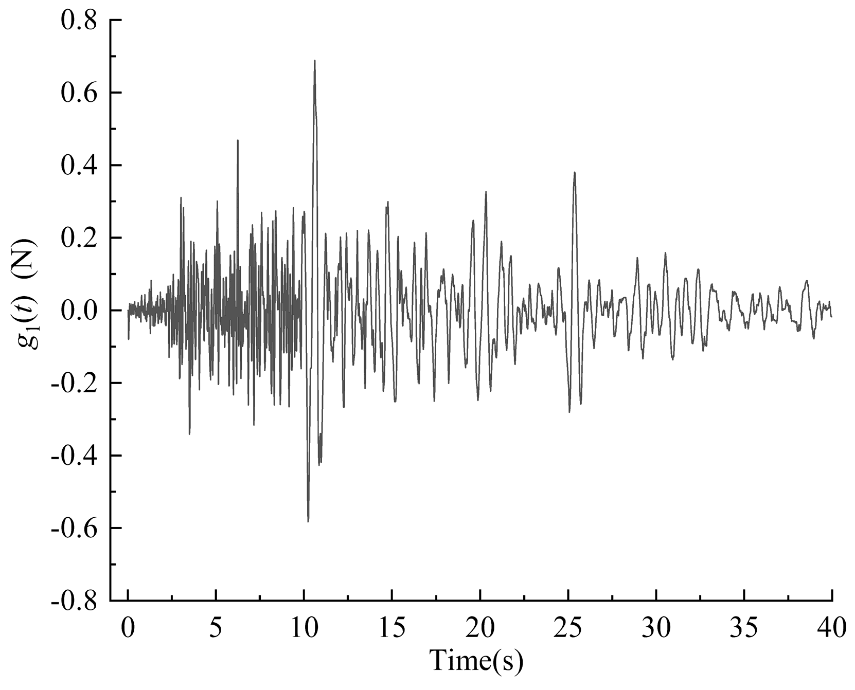
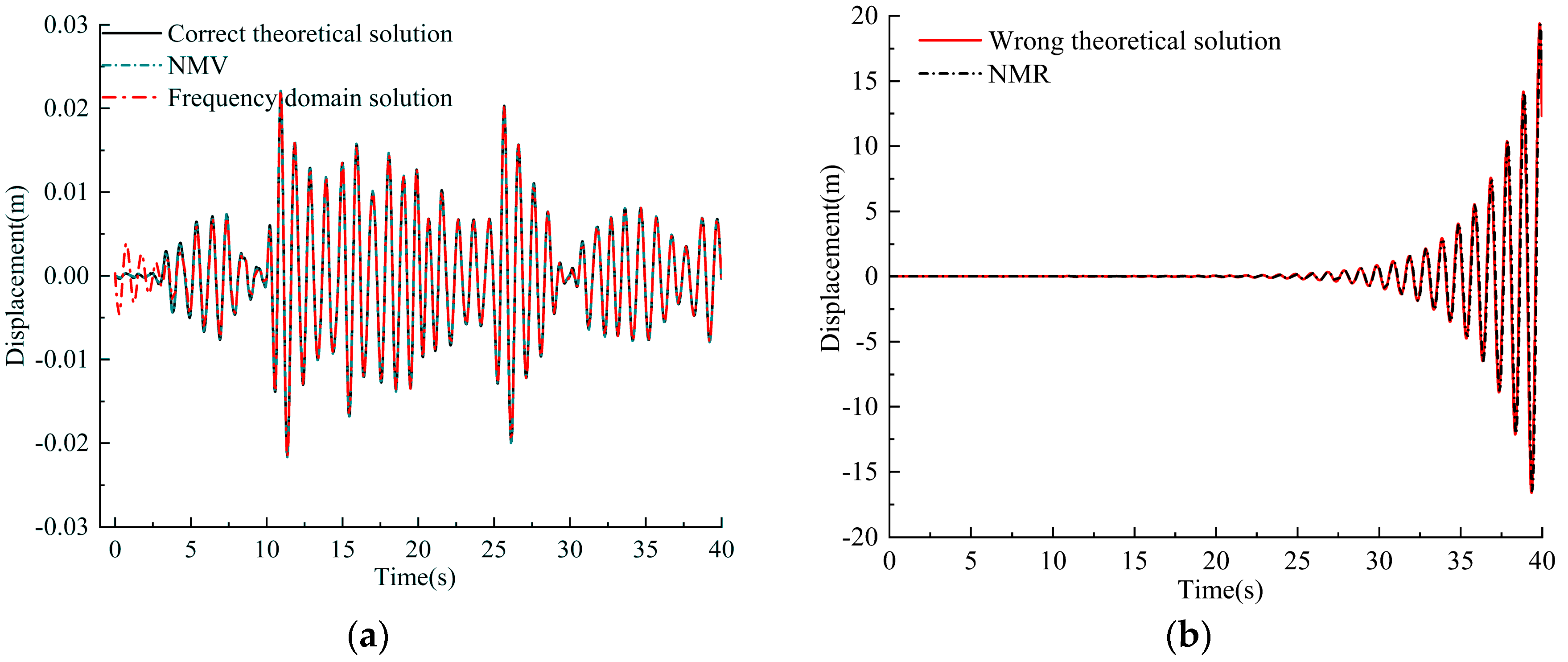
4.3. Seismic Excitation

This example case study analyzed an SDOF with m = 1, k = 4π², and η = 0.1 subjected to seismic excitation with ground acceleration ${\ddot{u}}_g(t)$. The equivalent real-valued force g₁(t) is

$$g_1(t)=-m{\ddot{u}}_g(t).$$

(52)

In this example, acceleration ${\ddot{u}}_g(t)$ was the ground motion recorded at a site in Whittier Narrows, California during the Whittier earthquake of 1 October 1987. The force g₁(t) is shown in Figure 3.

Figure 4a compares the proposed Newmark method with virtual initial conditions with the correct theoretical solution by Equation (41) and the frequency domain method, and Figure 4b shows the Newmark method with the real-valued initial conditions (NMR) and the wrong solution by Equation (40) with the real initial conditions. The Newmark method’s parameters are $\gamma =\frac{1}{2}$, $\beta =\frac{1}{4}$, and the integration time interval is $\Delta t=0.02s$.

Figure 4a,b further confirm that the divergence of the numerical solution is caused by the divergent term of complementary solution. The Newmark method would converge to the wrong theoretical solution for initial conditions $u_0=0$ and $v_0=0$. However, after introducing the virtual initial conditions, the Newmark method would converge to the correct theoretical solution. The difference between the NMV and frequency domain method is in the initial stage. Therefore, the frequency domain method would obtain reasonable results if the response is relatively small at the beginning of vibration.

5. Conclusions

In this paper, a direct integration virtual initial conditions method is developed for the numerical solution of the free or forced vibration of a hysteretic damped system. Based on extensive theoretic derivations and numerical analysis, the following conclusions can be drawn:

(1)

For free or forced vibration of a hysteretic damped system, the stability of numerical methods is the same as that of a viscously damped system. The divergence of numerical results is caused by the divergent term of the complementary solution if using the real-valued initial conditions. The virtual initial conditions can remove the divergent term, and make the numerical solution converge to the exact theoretical solution.

(2)

The virtual initial conditions are purely imaginary. For free vibration, the virtual initial conditions depend on the real-valued initial conditions, and for forced vibration, the virtual initial conditions depend on the amplitude of the force.

(3)

The solution in the frequency domain can only obtain the steady-state vibration. However, the proposed direct integration method can accurately calculate the transient response, which results in a reasonable estimation for whole vibration history and is, thus, recommended for practical applications.

In the future, the direct integration virtual initial conditions method is recommended to be further developed for the multi-degree-of-freedom system with hysteretic damping and non-linear dynamic response.

References

1. Chopra, A.K. Dynamics of Structures: Theory and Applications to Earthquake Engineering; Prentice-Hall: Englewood Cliffs, NJ, USA, 1995. [Google Scholar]
2. Bert, C.W. Material damping: An introductory review of mathematical models, measures, and experimental techniques. J. Sound Vib. 1973, 29, 129–153. [Google Scholar] [CrossRef]
3. Lazan, B.J. Damping of Material and Members in Structural Mechanics; Pergamon Press: London, UK, 1968. [Google Scholar]
4. Rinaldin, G.; Amadio, C.; Fragiacomo, M. Effects of seismic sequences on structures with hysteretic or damped dissipative behaviour. Soil Dyn. Earthq. Eng. 2017, 97, 205–215. [Google Scholar] [CrossRef]
5. Maiti, S.; Bandyopadhyay, R.; Chatterjee, A. Vibrations of an Euler-Bernoulli beam with hysteretic damping arising from dispersed frictional microcracks. J. Sound Vib. 2018, 412, 287–308. [Google Scholar] [CrossRef]
6. Zhou, L.; Su, Y.S. Cyclic Loading Test on Beam-to-Column Connections Connecting SRRAC Beams to RACFST Columns. Int. J. Civ. Eng. 2018, 16, 1533–1548. [Google Scholar] [CrossRef]
7. Sheng, M.; Guo, Z.; Qin, Q.; He, Y. Vibration characteristics of a sandwich plate with viscoelastic periodic cores. Compos. Struct. 2018, 206, 54–69. [Google Scholar] [CrossRef]
8. Martakis, P.; Taeseri, D.; Chatzi, E.; Laue, J. A centrifuge-based experimental verification of Soil-Structure Interaction effects. Soil Dyn. Earthq. Eng. 2017, 103, 1–14. [Google Scholar] [CrossRef]
9. Singiresu, S.R. Mechanical Vibrations; Addison-Wesley Publishing Company: New York, NY, USA, 1990. [Google Scholar]
10. Pavlou, E.A. Dynamic Analysis of Systems with Hysteretic Damping; Rice University: Houston, TX, USA, 1999. [Google Scholar]
11. Chakraborty, G. On Response of a Single-Degree-of-Freedom Oscillator with Constant Hysteretic Damping Under Arbitrary Excitation. J. Inst. Eng. (India) Ser. C 2016, 97, 579–582. [Google Scholar] [CrossRef]
12. Lacayo, R.; Pesaresi, L.; Groß, J.; Fochler, D.; Armand, J.; Salles, L.; Schwingshack, C.; Allen, M.; Brake, M. Nonlinear modeling of structures with bolted joints: A comparison of two approaches based on a time-domain and frequency-domain solver. Mech. Syst. Signal Process. 2019, 114, 413–438. [Google Scholar] [CrossRef] [Green Version]
13. Schriefer, T.; Hofmann, M. A hybrid frequency-time-domain approach to determine the vibration fatigue life of electronic devices. Microelectron. Reliab. 2019, 98, 86–94. [Google Scholar] [CrossRef]
14. Idriss, I.M.; Seed, H.B. Seismic response of horizontal soil layers. J. Soil Mech. Found. Div. 1968, 94, 1003–1031. [Google Scholar]
15. Star, L.M.; Tileylioglu, S.; Givens, M.J.; Mylonakis, G.; Stewart, J.P. Evaluation of soil-structure interaction effects from system identification of structures subject to forced vibration tests. Soil Dyn. Earthq. Eng. 2019, 116, 747–760. [Google Scholar] [CrossRef]
16. Khodakarami, M.I.; Lashgari, A. An equivalent linear substructure approximation for the analysis of the liquefaction effects on the dynamic soil–structure interaction. Asian J. Civ. Eng. 2018, 19, 67–78. [Google Scholar] [CrossRef]
17. Nampally, S.; Padhy, S.; Trupti, S.; Prasad, P.P.; Seshunarayana, T. Evaluation of site effects on ground motions based on equivalent linear site response analysis and liquefaction potential in Chennai, South India. J. Seismol. 2018, 22, 1075–1093. [Google Scholar] [CrossRef]
18. Sonmezer, Y.B.; Bas, S.; Isik, N.S.; Akbas, S.O. Linear and nonlinear site response analyses to determine dynamic soil properties of Kirikkale. Geomech. Eng. 2018, 16, 435–448. [Google Scholar] [CrossRef]
19. Clough, R.W.; Penzien, J. Dynamics of Structures; McGraw-Hill: New York, NY, USA, 1975; pp. 194–198. [Google Scholar]
20. Poul, M.K.; Zerva, A. Efficient time-domain deconvolution of seismic ground motions using the equivalent-linear method for soil-structure interaction analyses. Soil Dyn. Earthq. Eng. 2018, 112, 138–151. [Google Scholar] [CrossRef]
21. Liang, F.; Chen, H.; Huang, M. Accuracy of three-dimensional seismic ground response analysis in time domain using nonlinear numerical simulations. Earthq. Eng. Eng. Vib. 2017, 32–43. [Google Scholar] [CrossRef]
22. Coleman, J.; Bolisetti, C.; Whittaker, A. Time-domain soil-structure interaction analysis of nuclear facilities. Nucl. Eng. Des. 2016, 298, 264–270. [Google Scholar] [CrossRef] [Green Version]
23. Rostami, S.; Shojaee, S. Development of a Direct Time Integration Method Based on Quartic B-spline Collocation Method. Iran. J. Sci. Technol. Trans. Civ. Eng. 2019, 43 (Suppl. 1), 615–636. [Google Scholar] [CrossRef]
24. Zhu, M.; Zhu, J. Studies on stability of step-by-step methods under complex damping conditions. Earthq. Eng. Eng. Vib. 2001, 21, 59–62. (In Chinese) [Google Scholar] [CrossRef]
25. Henwood, D.J. Approximating the Hysteretic Damping Matrix by a Viscous Matrix for Modelling in the Time Domain. J. Sound Vib. 2002, 254, 575–593. [Google Scholar] [CrossRef]
26. Chen, J.T.; You, D.W. An integral–differential equation approach for the free vibration of a SDOF system with hysteretic damping. Adv. Eng. Softw. 1999, 30, 43–48. [Google Scholar] [CrossRef]
27. Zhou, Z.; Liao, Z.; Ding, H. A time-domain complex-damping constitutive equation. Earthq. Eng. Eng. Vib. 1999, 19, 37–44. (In Chinese) [Google Scholar] [CrossRef]
28. Sun, P.; Yang, H.; Zhao, W.; Liu, Q. The time-domain numerical calculation method based on complex damping model. Earthq. Eng. Eng. Vib. 2019, 39, 203–211. (In Chinese) [Google Scholar] [CrossRef]
29. Ribeiro, A.M.R.; Maia, N.M.M.; Silva, J.M.M. Free and Forced Vibration with Viscous and Hysteretic Damping: A Different Perspective. In Proceedings of the 5th International Conference on Mechanics and Materials in Design, Porto, Portugal, 24–26 July 2006. [Google Scholar] [CrossRef]
30. Zhu, M.; Zhu, J. Some problems in frequency domain solution of complex damping system. World Earthq. Eng. 2004, 1, 23–28. (In Chinese) [Google Scholar] [CrossRef]
Figure 1. Free vibration solutions.
Applsci 09 03707 g001
Figure 2. Forced vibration solution with harmonic force.
Applsci 09 03707 g002
Figure 3. Equivalent real-valued force g1(t).
Applsci 09 03707 g003
Figure 4. Forced vibration solution with arbitrary loading: (a) correct theoretical solution, NMV, frequency domain solution; (b) wrong theoretical solution and NMR.
Applsci 09 03707 g004