Weak Fault Feature Extraction and Enhancement of Wind Turbine Bearing Based on OCYCBD and SVDD


Abstract
:1. Introduction
2. Optimized Cyclostationary Blind Deconvolution
2.1. Theoretical Background of Cyclostationary Blind Deconvolution
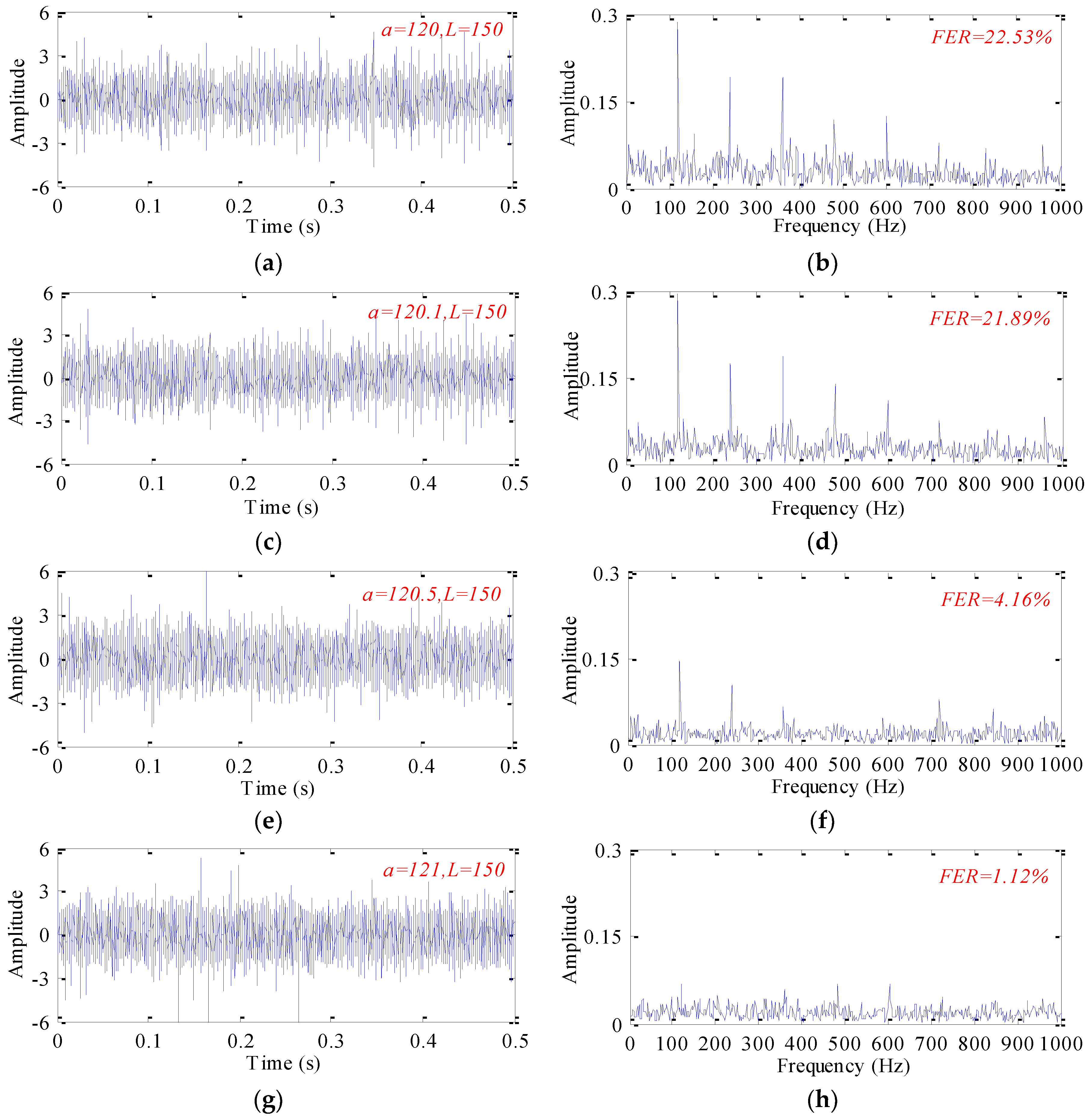
2.2. Research on the Influences of Key Parameters
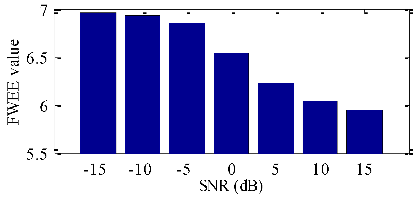
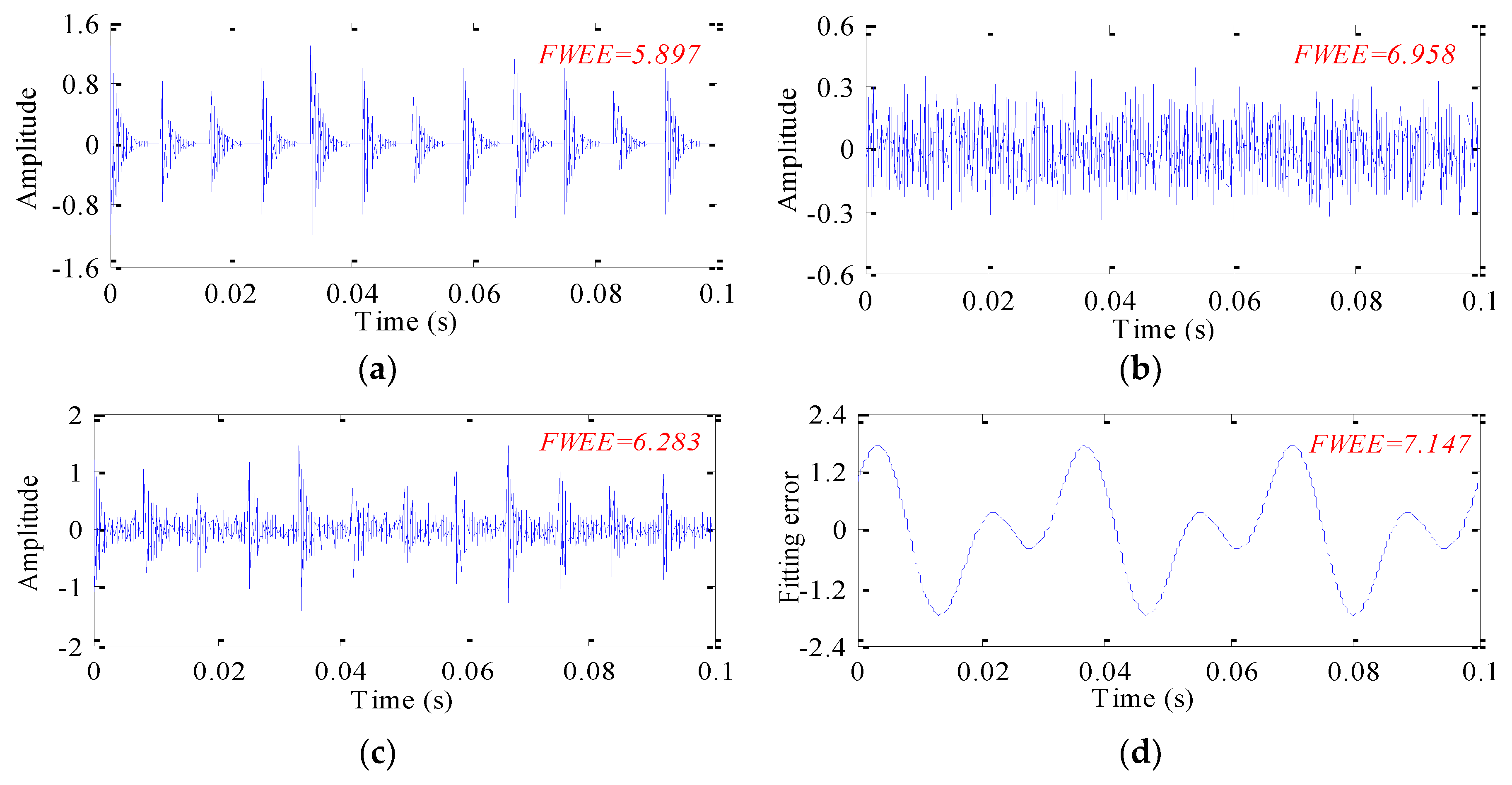
2.3. Frequency Weighted Energy Entropy Indicator
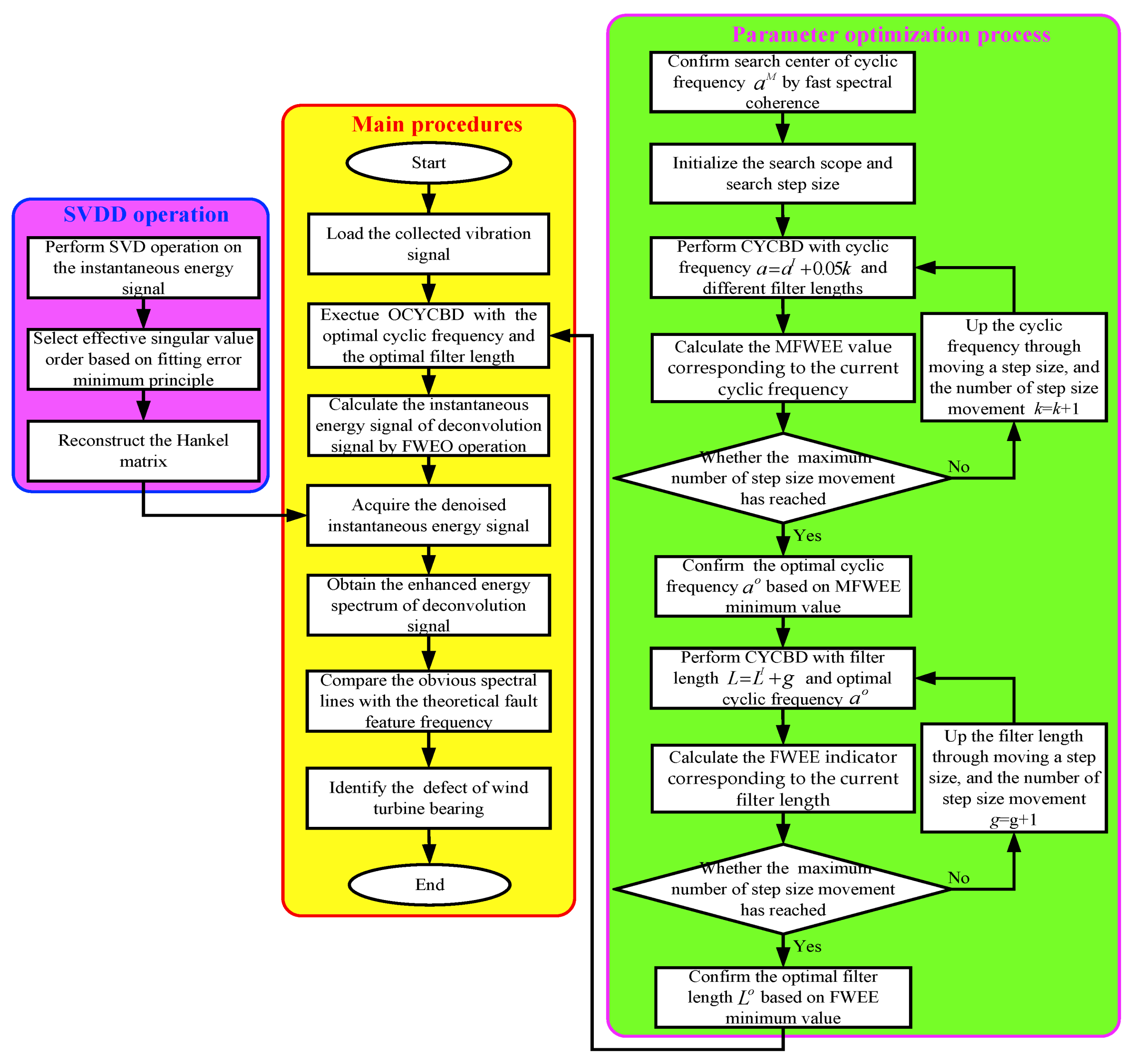
2.4. Optimal Parameter Selection Stragegy Guided by FWEE Indicator
- Step 1
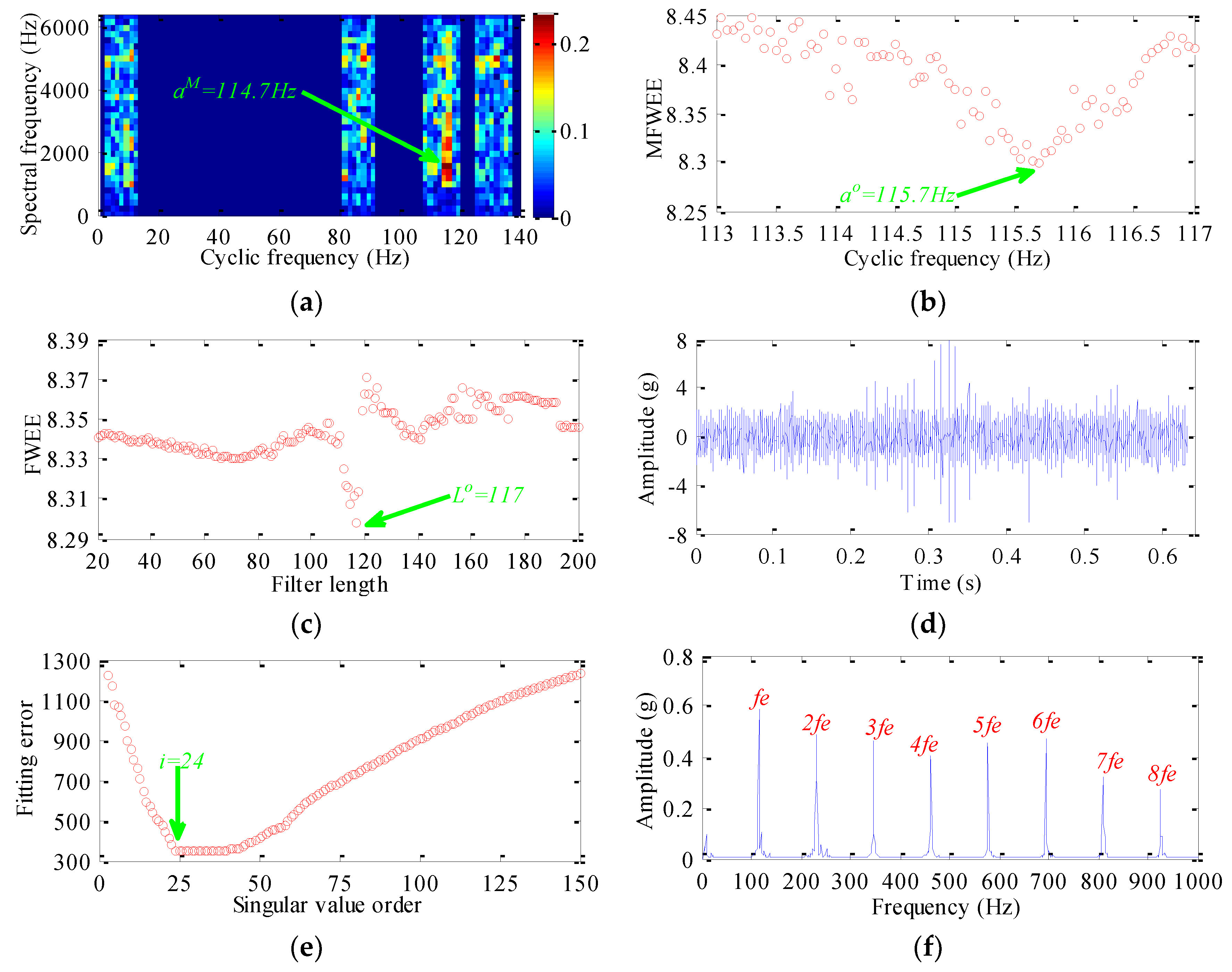
- Confirm the search center of cyclic frequency. It is a great challenge to determinate the cyclic frequency parameter with a high precision owing to the wide search scope. Thus, for the purpose of improving the search efficiency and easing the computational burden, the search center of cyclic frequency needs to be confirmed firstly, and the whole search process is carried out around this center. Spectral coherence provides a new interpretation of periodic flows of energy across the analysis frequency band and the cyclic frequency band [27]. With the help of its excellent ability in revealing the presence of modulation and describing the cyclostationarity, the fast spectral coherence is applied to accurately estimate the search center, and the relevance theory of fast spectral coherence can refer to literature [28]. The cyclic frequency location corresponding to the maximum energy distribution in the fast spectral coherence is regarded as the search center . In order to avoid the interference as far as possible, only the regions [, ] () around the theoretical defect feature frequencies are analyzed, where , , and respectively represent the theoretical defect feature frequencies of inner ring, outer ring, roller, and cage. In this paper, the analysis region interval is set to 5Hz. However, the precise cyclic frequency parameter is still difficult to determinate due to the influence of cyclic frequency resolution. Then more precise search process around the search center is performed in the following steps.
- Step 2
- Determinate the search scope and search step size. The search scope of cyclic frequency parameter is initialized as [, ] = [floor(), ceil()] with search step size of 0.05Hz. Where and are the upper boundary and the lower boundary of search scope, denotes the cyclic frequency resolution of spectral coherence, floor and ceil respectively refer to the round down operation and the round up operation. As for the filter length , the deconvolution signal will be distorted if it is too large, while the treatment efficiency will be inconspicuous if this parameter is too small. Referring to literature [15], the search scope of filter length is set as [, ] = [20,200] with search step size of 1, where and denote the upper boundary and the lower boundary of search scope.
- Step 3
- Determinate the optimal cyclic frequency parameter. In the circumstances of different values, the mean of frequency weighted energy entropy (MFWEE) is calculated to select the optimal cyclic frequency . When = , the different filter lengths = [20,40,60,,200] are respectively substituted into CYCBD, and the corresponding 10 set of deconvolution signals are obtained. Then the FWEE indicator of each deconvolution signal is calculated and the mean of 10 FWEE indicators corresponding to can be acquired. For (k = 0,1,2,, is the number of step size movement), the MFWEE value corresponding to each cyclic frequency is in turn calculated based on the similar process. And all MFWEE values corresponding to the whole search scope [floor (), ceil ()] can be obtained. If the MFWEE value is smaller, then it means the periodic impact signature in the obtained deconvolution signal is more prominent and the contained useful information is richer. Thus, during the process of key parameter optimization, the cyclic frequency corresponding to the MFWEE minimum value is regarded as the optimal parameter , then store this optimal parameter in the memory.
- Step 4
- Select the optimal filter length parameter. In order to further optimize the filter length on the basis of = , = [20,21,22,,200] are substituted into CYCBD respectively, and the corresponding 181 set of deconvolution signals are obtained, then the FWEE indicator of each deconvolution signal is calculated to evaluate the filter length parameter. For (g = 0,1,2,, is the number of step size movement), the FWEE indicator corresponding to each filter length is in turn calculated based on the similar process. And all FWEE indicators corresponding to the whole search scope [20,200] can be obtained. Then confirm the optimal filter length parameter when FWEE indicator is the smallest.
3. Singular Value Decomposition Denoising
3.1. Basic Theory of Singular Value Decomposition
3.2. Singular Value Order Determination
- (1)
- The singular value sequence and the order sequence are obtained by applying SVD to the given signal using Equations (22) and (23). The first singular value, which corresponding the trend component of the signal, is obvious larger than the others in the singular value sequence. In order to avoid causing large deviation, then the first singular value is removed in the whole process.
- (2)
- The initial order r is confirmed.
- (3)
- According to the order r, the original singular value sequence is split into two set of sequences and , and the original order sequence is also split into two set of sequences and .
- (4)
- The order sequences and are respectively considered as the independent variables and the singular value sequences and are respectively regarded as the dependent variables. Then the least squares quadratic polynomial fitting method is utilized to construct the fitting function and . Where , , , , and are the polynomial coefficients, and are the independent variables.
- (5)
- The fitting error corresponding to the order r is calculated by the following expression: .
- (6)
- The order r is reassigned as r = r + 1.
- (7)
- The steps (3)–(6) are repetitive executed until r = p.
- (8)
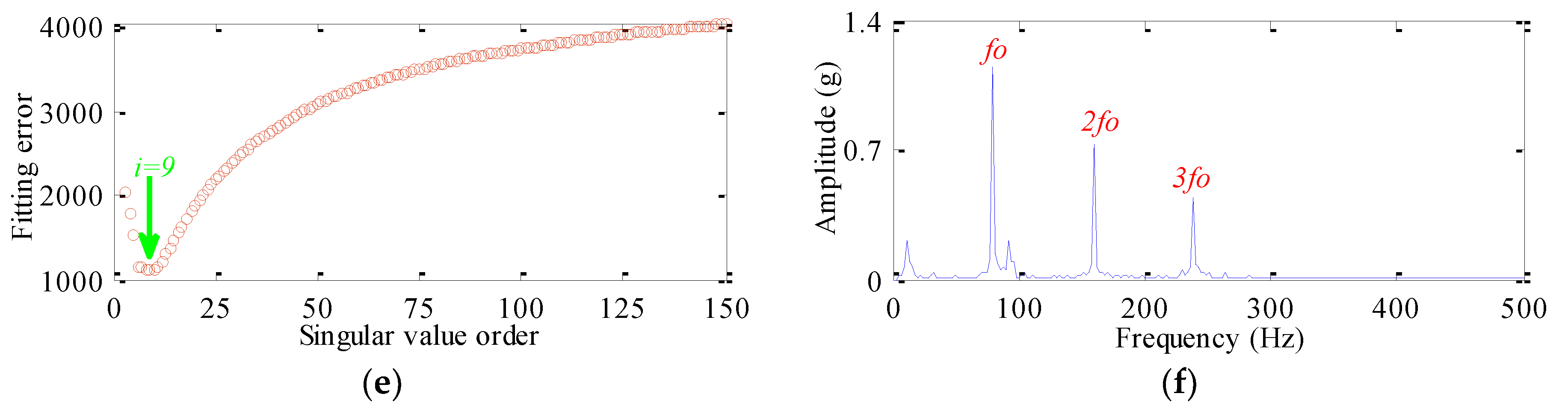
- The minimum value of fitting error is confirmed, then the corresponding order i is regarded as the diacritical location of the available and the useless singular values. And the former i singular values except for the first one are applied for purified signal reconstruction.
4. Fault Feature Extraction and Enhancement Method Based on OCYCBD and SVDD
- (1)
- Data acquisition. The original signal is collected using the corresponding data acquire equipments.
- (2)
- OCYCBD processing. The fast spectral coherence and the equal step size search strategy are combined organically to search for the optimal cycle frequency and the filter length, and the corresponding steps have been elaborate explained in Section 2.4. The obtained optimal parameters are substituted into CYCBD. Then the informative fault source with higher SNR can be recovered from the original collected signal by deconvolution operation.
- (3)
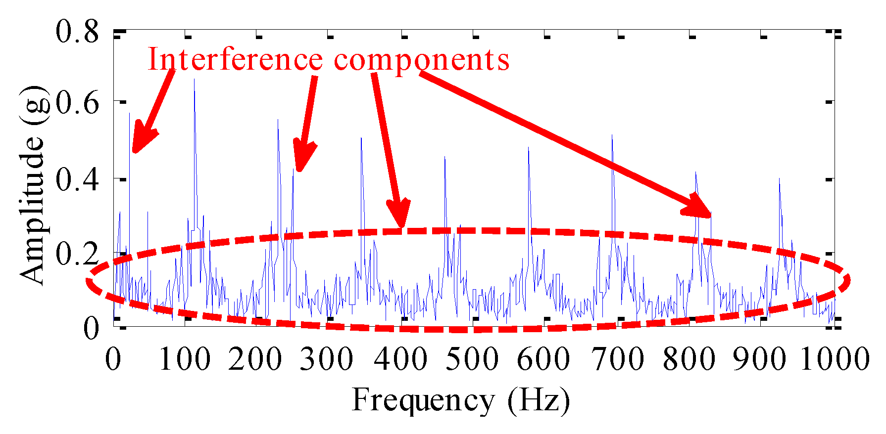
- Instantaneous energy signal calculation. The FWEO operation is carried out on the obtained deconvolution signal to calculate the instantaneous energy signal. The impulsive signature of the instantaneous energy signal is more outstanding than the original signal, but there still exist the interference components. Then the following procedure is carried out to get rid of the redundant components in the instantaneous energy signal and enhance the defect signature.
- (4)
- SVDD processing. The SVDD approach is further utilized for instantaneous energy signal denoising. And the effective singular value order to reconstruct the matrix can be determined using the fitting error minimum principle. Because the quadratic polynomial fitting algorithm is utilized to establish the fitting functions, thus the initial order is set to r = 4. And the denoised instantaneous energy signal can be gained through the diagonal mean operation of reconstructed matrix.
- (5)
- Enhanced energy spectrum analysis. The Fourier transform based spectrum analysis is performed on the purified instantaneous energy signal of deconvolution signal, and the corresponding enhanced energy spectrum of deconvolution signal can be acquired. Then the defect location of wind turbine bearing is able to be judged by analyzing the spectral peak in the enhanced energy spectrum.
5. Experiment Verification
5.1. Introduction of Experimental Platform
5.2. Experimental Signal Analysis and Result Comparsion
6. Engineering Case Verification
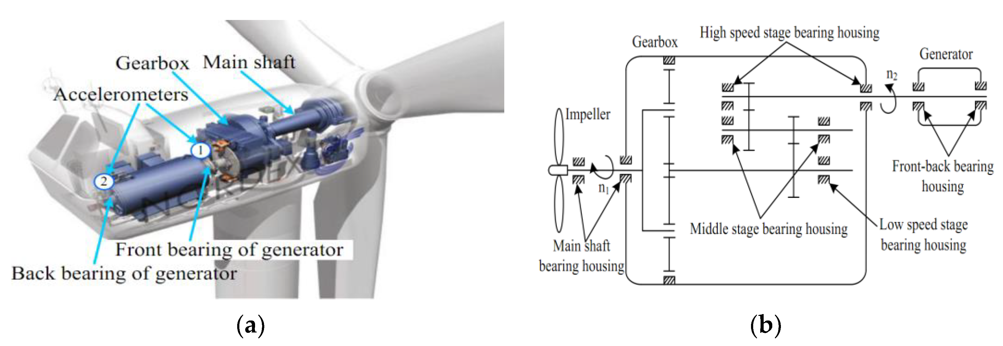
6.1. Description of Wind Turbine
6.2. Engineering Signal Analysis and Result Comparsion
7. Conclusions
- (1)
- The influences of the cyclic frequency and the filter length on the performance of CYCBD are researched by the simulated fault signal. In addition, the FWEE indicator, which can effectively reflect the richness of periodic impact component, is proposed to evaluate the quality of deconvolution signal during parameter optimization process.
- (2)
- The OCYCBD method fusing the fast spectral coherence with the equal step size search strategy is put forward to overcome the drawback of CYCBD, by which the optimal deconvolution result can be achieved automatically.
- (3)
- A novel fitting error minimum principle is used by SVDD to select the effective singular value order, the redundant interferences can be suppressed and the fault feature can be enhanced tremendously through denoising operation.
Author Contributions
Funding
Acknowledgments
Conflicts of Interest
Abbreviations
| WVD | wigner ville distribution |
| WT | wavelet transform |
| EMD | empirical mode decomposition |
| SK | spectral kurtosis |
| SNR | signal to noise ratio |
| MED | minimum entropy deconvolution |
| MCKD | maximum correlated kurtosis deconvolution |
| CYCBD | cyclostationary blind deconvolution |
| OCYCBD | optimized cyclostationary blind deconvolution |
| SVDD | singular value decomposition denoising |
| SVD | singular value decomposition |
| FER | feature energy ratio |
| FWEO | frequency weighted energy operator |
| FWEE | frequency weighted energy entropy |
| MFWEE | mean of frequency weighted energy entropy |
References
- Inturi, V.; Sabareesh, G.R.; Supradeepan, K.; Penumakala, P.K. Integrated condition monitoring scheme for bearing fault diagnosis of a wind turbine gearbox. J. Vib. Control 2019, 25, 1852–1865. [Google Scholar] [CrossRef]
- Wang, Z.J.; Wang, J.Y.; Kou, Y.F.; Zhang, J.P.; Ning, S.H.; Zhao, Z.F. Weak fault diagnosis of wind turbine gearboxes based on MED-LMD. Entropy 2017, 19, 277. [Google Scholar] [CrossRef]
- Zhang, J.; Zhang, J.Q.; Zhong, M.; Zhong, J.H.; Zheng, J.D.; Yao, L.G. Detection for incipient damages of wind turbine bolling bearing based on VMD-AMCKD method. IEEE Access 2019, 7, 67944–67959. [Google Scholar] [CrossRef]
- Miao, Y.H.; Zhao, M.; Lin, J.; Xu, X.Q. Sparse maximum harmonics-to-noise-ratio deconvolution for weak fault signature detection in bearings. Meas. Sci. Technol. 2016, 27, 1–17. [Google Scholar] [CrossRef]
- Yan, X.A.; Jia, M.P.; Zhao, J.Z. A novel intelligent detection method for rolling bearing based on IVMD and instantaneous energy distribution-permutation entropy. Measurement 2018, 130, 435–447. [Google Scholar] [CrossRef]
- Sharma, R.R.; Pachori, R.B. Improved eigenvalue decomposition-based approach for reducing cross-terms in wigner-ville distribution. Circuits Syst. Signal Process. 2018, 37, 3330–3350. [Google Scholar] [CrossRef]
- Wang, X.L.; Tang, G.J.; Zhou, F.C. Application of adaptive tunable Q-factor wavelet transform on incipient fault diagnosis of bearing. J. Aerosp. Power 2017, 32, 2467–2475. [Google Scholar]
- Wang, X.L.; Zhou, F.C.; He, Y.L.; Wu, Y.J. Weak fault diagnosis of rolling bearing under variable speed condition using IEWT-based enhanced envelope order spectrum. Meas. Sci. Technol. 2019, 30, 1–18. [Google Scholar] [CrossRef]
- Wan, S.T.; Peng, B. Adaptive asymmetric real laplace wavelet filtering and its application on rolling bearing early fault diagnosis. Shock Vib. 2019, 2019, 7475868. [Google Scholar] [CrossRef]
- Jiang, R.L.; Chen, J.; Dong, G.M.; Liu, T.; Xiao, W.B. The weak fault diagnosis and condition monitoring of rolling element bearing using minimum entropy deconvolution and envelop spectrum. Proc. Inst. Mech. Eng. Part C J. Mech. Eng. Sci. 2013, 227, 1116–1129. [Google Scholar] [CrossRef]
- Wang, Z.J.; Zhou, J.; Wang, J.Y.; Du, W.H.; Wang, J.T.; Han, X.F.; He, G.F. A novel fault diagnosis method of gearbox based on maximum kurtosis spectral entropy deconvolution. IEEE Access 2019, 7, 29520–29532. [Google Scholar] [CrossRef]
- McDonald, G.L.; Zhao, Q.; Zuo, M.J. Maximum correlated kurtosis deconvolution and application on gear tooth chip fault detection. Mech. Syst. Signal Process. 2012, 33, 237–255. [Google Scholar] [CrossRef]
- Jia, F.; Lei, Y.G.; Shan, H.K.; Lin, J. Early fault diagnosis of bearings using an improved spectral kurtosis by maximum correlated kurtosis deconvolution. Sensors 2015, 15, 29363–29377. [Google Scholar] [CrossRef] [PubMed]
- Cui, L.L.; Du, J.X.; Yang, N.; Xu, Y.G.; Song, L.Y. Compound faults feature extraction for rolling bearings based on parallel dual-Q-factors and the improved maximum correlated kurtosis deconvolution. Appl. Sci. 2019, 9, 1681. [Google Scholar] [CrossRef]
- Buzzoni, M.; Antoni, J.; D’Elia, J. Blind deconvolution based on cyclostationarity maximization and its application to fault identification. J. Sound Vib. 2018, 432, 569–601. [Google Scholar] [CrossRef]
- Zhao, H.S.; Li, L. Fault diagnosis of wind turbine bearing based on variational mode decomposition and Teager energy operator. IET Renew. Power Gener. 2017, 11, 453–460. [Google Scholar] [CrossRef]
- Cai, Z.Y.; Xu, Y.B.; Duan, Z.S. An alternative demodulation method using envelope-derivative operator for bearing fault diagnosis of the vibrating screen. J. Vib. Control 2018, 24, 3249–3261. [Google Scholar] [CrossRef]
- O’Toole, J.M.; Temko, A.; Stevenson, N. Assessing instantaneous energy in the EEG: A non-negative, frequency-weighted energy operator. In Proceedings of the 36th Annual International Conference of the IEEE Engineering in Medicine and Biology Society, Chicago, IL, USA, 26–30 August 2014; pp. 3288–3291. [Google Scholar]
- Imaouchen, Y.; Kedadouche, M.; Alkama, R.; Thomas, M. A frequency-weighted energy operator and complementary ensemble empirical mode decomposition for bearing fault detection. Mech. Syst. Signal Process. 2017, 82, 103–116. [Google Scholar] [CrossRef]
- Pang, B.; He, Y.L.; Tang, G.J.; Zhou, C.; Tian, T. Rolling bearing fault diagnosis based on optimal notch filter and enhanced singular value decomposition. Entropy 2018, 20, 482. [Google Scholar] [CrossRef]
- Liao, Y.H.; Sun, P.; Wang, B.X.; Qu, L. Extraction of repetitive transients with frequency domain multipoint kurtosis for bearing fault diagnosis. Meas. Sci. Technol. 2018, 29, 1–12. [Google Scholar] [CrossRef]
- Yan, X.A.; Jia, M.P. Application of CSA-VMD and optimal scale morphological slice bispectrum in enhancing outer race fault detection of rolling element bearings. Mech. Syst. Signal Process. 2019, 122, 56–86. [Google Scholar] [CrossRef]
- Tian, X.G.; Gu, J.X.; Rehab, I.; Abdalla, G.M.; Gu, F.S.; Ball, A.D. A robust detector for rolling element bearing condition monitoring based on the modulation signal bispectrum and its performance evaluation against the Kurtogram. Mech. Syst. Signal Process. 2018, 100, 167–187. [Google Scholar] [CrossRef]
- Tang, G.J.; Wang, X.L.; He, Y.L. Diagnosis of compound faults of rolling bearings through adaptive maximum correlated kurtosis deconvolution. J. Mech. Sci. Technol. 2016, 30, 43–54. [Google Scholar] [CrossRef]
- Xu, Y.B.; Cai, Z.Y.; Hu, Y.B.; Ding, K. A frequency-weighted enemy operator and variational mode decomposition for bearing fault detection. J. Vib. Eng. 2018, 31, 513–522. [Google Scholar]
- Wan, S.T.; Zhang, X.; Dou, L.J. Shannon entropy of binary wavelet packet subbands and its application in bearing fault extraction. Entropy 2018, 20, 388. [Google Scholar] [CrossRef]
- Tang, G.J.; Pang, B.; Tian, T.; Zhou, C. Fault diagnosis of rolling bearings based on improved fast spectral correlation and optimized random forest. Appl. Sci. 2018, 8, 1859. [Google Scholar] [CrossRef]
- Antoni, J.; Xin, G.; Hamzaoui, N. Fast computation of the spectral correlation. Mech. Syst. Signal Process. 2017, 92, 248–277. [Google Scholar] [CrossRef]
- Ren, Y.; Li, W.; Zhu, Z.C.; Jiang, F. ISVD-based in-band noise reduction approach combined with envelope order analysis for rolling bearing vibration monitoring under varying speed conditions. IEEE Access 2019, 7, 32072–32084. [Google Scholar] [CrossRef]
- Ma, J.; Wu, J.D.; Wang, X.D. A hybrid fault diagnosis method based on singular value difference spectrum denoising and local mean decomposition for rolling bearing. J. Low Freq. Noise Vib. Act. Control 2018, 37, 928–954. [Google Scholar] [CrossRef]
- Wang, Y.Y. Mean value of eigenvalue based SVD signal denoising algorithm. Comput. Appl. Softw. 2012, 29, 121–124. [Google Scholar]
- Laha, S.K. Enhancement of fault diagnosis of rolling element bearing using maximum kurtosis fast nonlocal means denoising. Measurement 2017, 100, 157–163. [Google Scholar] [CrossRef]


| Number of Balls | Diameter of Balls (mm) | Pitch Diameter (mm) | Contact Angle (°) |
|---|---|---|---|
| 9 | 7.94 | 39.04 | 0 |
| Number of Balls | Diameter of Balls (mm) | Pitch Diameter (mm) | Contact Angle (°) |
|---|---|---|---|
| 8 | 41.275 | 190 | 0 |
© 2019 by the authors. Licensee MDPI, Basel, Switzerland. This article is an open access article distributed under the terms and conditions of the Creative Commons Attribution (CC BY) license (http://creativecommons.org/licenses/by/4.0/).
Share and Cite
Wang, X.; Yan, X.; He, Y. Weak Fault Feature Extraction and Enhancement of Wind Turbine Bearing Based on OCYCBD and SVDD. Appl. Sci. 2019, 9, 3706. https://doi.org/10.3390/app9183706
Wang X, Yan X, He Y. Weak Fault Feature Extraction and Enhancement of Wind Turbine Bearing Based on OCYCBD and SVDD. Applied Sciences. 2019; 9(18):3706. https://doi.org/10.3390/app9183706
Chicago/Turabian StyleWang, Xiaolong, Xiaoli Yan, and Yuling He. 2019. "Weak Fault Feature Extraction and Enhancement of Wind Turbine Bearing Based on OCYCBD and SVDD" Applied Sciences 9, no. 18: 3706. https://doi.org/10.3390/app9183706
APA StyleWang, X., Yan, X., & He, Y. (2019). Weak Fault Feature Extraction and Enhancement of Wind Turbine Bearing Based on OCYCBD and SVDD. Applied Sciences, 9(18), 3706. https://doi.org/10.3390/app9183706