Article

An Effective Surrogate Ensemble Modeling Method for Satellite Coverage Traffic Volume Prediction

1
College of Aerospace Science and Engineering, National University of Defense Technology, Changsha 410073, China
2
National Innovation Institute of Defense Technology, Chinese Academy of Military Science, Beijing 100000, China
*
Author to whom correspondence should be addressed.
Appl. Sci. 2019, 9(18), 3689; https://doi.org/10.3390/app9183689
Submission received: 8 July 2019 / Revised: 22 August 2019 / Accepted: 23 August 2019 / Published: 5 September 2019

Abstract

:
The satellite constellation network is a powerful tool to provide ground traffic business services for continuous global coverage. For the resource-limited satellite network, it is necessary to predict satellite coverage traffic volume (SCTV) in advance to properly allocate onboard resources for better task fulfillment. Traditionally, a global SCTV distribution data table is first statistically constructed on the ground according to historical data and uploaded to the satellite. Then SCTV is predicted onboard by a data table lookup. However, the cost of the large data transmission and storage is expensive and prohibitive for satellites. To solve these problems, this paper proposes to distill the data into a surrogate model to be uploaded to the satellite, which can both save the valuable communication link resource and improve the SCTV prediction accuracy compared to the table lookup. An effective surrogate ensemble modeling method is proposed in this paper for better prediction. First, according to prior geographical knowledge of the SCTV distribution, the global earth surface domain is split into multiple sub-domains. Second, on each sub-domain, multiple candidate surrogates are built. To fully exploit these surrogates and combine them into a more accurate ensemble, a partial weighted aggregation method (PWTA) is developed. For each sub-domain, PWTA adaptively selects the candidate surrogates with higher accuracy as the contributing models, based on which the ultimate ensemble is constructed for each sub-domain SCTV prediction. The proposed method is demonstrated and testified with an air traffic SCTV engineering problem. The results demonstrate the effectiveness of PWTA regarding good local and global prediction accuracy and modeling robustness.

1. Introduction

In recent decades, satellite constellation networks have been developed to provide multiple ground traffic services for continuous global coverage, which can effectively supplement the coverage-limited terrestrial networks, such as air traffic monitoring [1] and ship trajectory identification [2]. Since the traffic distribution is geographically non-uniform, e.g., aircraft traffic distribution is dense in population agglomeration while scarce in vast ocean regions, satellite coverage traffic volume (SCTV) changes drastically during the satellite movement. To better fulfill the ground traffic service task, it is necessary to predict SCTV in advance so that the resource-limited satellite network could allocate the onboard resources dynamically, e.g., provide more power for payloads to work with full capacity. With the auxiliary information of the predicted upcoming ground traffic, He et al. [3] optimize the frequency reuse and onboard transmit power. Moreover, Yu et al. [4] adaptively adjust the onboard receiver configuration to improve the overall signal detection probability. To predict SCTV, traditionally a global SCTV distribution data table is first statistically constructed on the ground according to historical data and uploaded to the satellite. Then SCTV is predicted onboard by the data table lookup. To update the table with dynamically accumulated data, the SCTV data table should be uploaded each time the satellite passes over the ground station. Moreover, for better SCTV prediction, more data is preferred to construct a table with fine resolution. Then large data transmission and storage are necessitated, which is prohibitive for satellite communication and onboard data handling. To solve these problems, this paper proposes to distill the data into a surrogate model to be uploaded to satellite, which can both save the valuable communication link resource (as much fewer surrogate model parameters need be uploaded only) and improve the SCTV prediction accuracy compared to table lookup.
Recently, a surrogate modeling method, namely meta-modeling method, has been widely studied in data-driven modeling, mainly including Polynomial Response Surface (PRS) [5], Kriging [6,7], Radial Basis Function (RBF) [8], Support Vector Regression (SVR) [9], etc. In the work of Song et al. [10], the performance of PRS, RBF, Kriging, and SVR are compared in the design optimization of foam-filled tapered structures, and the results show that no single model is the best for approximating all objective functions in the considered problems. Forrester and Keane [11] review different meta-modeling methods used in surrogate-based optimization, and recommend that the choice of which surrogate to use should be based on the problem size, the expected complexity and the cost of the analyses. Similarly, Bhosekar et al. [12] investigate recent advances in the field of surrogate models for problems in modeling, feasibility analysis, and optimization. They conclude that the correct selection of surrogates should consider the type of problem at hand. From the previous research, the consensus is that each surrogate has its own superiorities and drawbacks, and different surrogates are suitable for approximating different objective functions [13]. For the SCTV prediction problem with geographically changing distribution features, as shown in the experimental study in Section 4, it is also observed that the single surrogate can hardly perform universally well in this problem.
To increase the approximation quality of the surrogate model, much research has been conducted into integrating multiple surrogates into a single ensemble to exploit the advantages of different surrogates for better approximation accuracy and robustness. One popular ensemble method is using the weighted sum approach [14]. Goel et al. [15] study the effectiveness of the weighted aggregation method for the approximation of helicopter vibrations. Wang et al. [16] employ the weighted average surrogate to solve the problem of computationally expensive function evaluations in optimization. Gu et al. [17] construct the ensemble of PRS, Kriging, RBF, and SVR for the approximation of an occupant protection system. For ensemble modeling, on one hand, the prediction accuracy of the ensemble is greatly influenced by the performance of the contributing surrogates. Viana et al. [18] find that adding inaccurate surrogates into the ensemble is likely to result in loss of accuracy. On the other hand, the weight factors also have a significant effect on the prediction accuracy of the ensemble. To obtain the ensemble with better performance, some research focuses on how to solve the appropriate weights considering the regional characteristics of the objective function to be approximated or predicted [19]. Zhang et al. [20] determine the weight of each contributing surrogate based on the local measure of accuracy in the pertinent trust region. Yin et al. [21] divide the design space into multiple sub-domains, each of which is assigned a set of optimized weights. These optimized weights are determined by minimizing the error metric of the training points in the corresponding sub-domains. Lee et al. [22] propose a pointwise ensemble which calculates the weights based on the v-nearest points cross-validation error. Although these studies could enhance the positive effects of the accurate contributing surrogates by increasing their weights in the local area, they do not completely eliminate the negative influences of the inaccurate contributing surrogates, leading to the relatively low accuracy of the ensemble model [23]. Moreover, for the SCTV prediction problem, the specific practical problem features should be considered for effective ensemble modeling.
In this paper, an effective surrogate ensemble modeling method is proposed for the SCTV prediction. First, the global earth surface domain is split into multiple sub-domains according to the prior geographical knowledge of the SCTV distribution, and then multiple different candidate surrogates are constructed on each sub-domain, respectively. Second, to fully exploit these surrogates and combine into a more accurate ensemble, a partial weighted aggregation method (PWTA) is developed. Because each sub-domain has distinct SCTV features, and different surrogates have different performance, PWTA adaptively selects the candidate surrogates with higher accuracy as the contributing models (the negative inaccurate surrogates are eliminated) for each sub-domain, based on which the ultimate ensemble is constructed in each sub-domain. In this way, for the sub-domains, there are independent positive contributing surrogates and weights so that the ensembles are more suitable for the corresponding sub-domains. Thus, the proposed surrogate ensemble modeling method could capture the regional SCTV features better in each sub-domain. The method proposed in this paper mainly has two contributions: (a) instead of constructing candidate surrogates in the global domain, multiple independent candidate surrogates are built for each sub-domain. (b) In each sub-domain, unlike integrating all the candidate surrogates to build an ensemble, the candidate surrogates are adaptively selected as contributing surrogates to construct a single ensemble.
The rest of the paper is organized as follows. In Section 2, a brief review of PRS, Kriging, RBF, the weighted aggregation method, and the BestGMSE surrogate are introduced. In Section 3, the satellite coverage traffic volume model is described, and the partial weighted surrogate ensemble modeling method is developed in detail. In Section 4, the proposed surrogate ensemble modeling method is testified in the SCTV prediction problem with engineering data, followed by the conclusions in the final section.

2. Preliminary

2.1. Polynomial Response Regression (PRS)

Suppose a deterministic function of m design variable has been evaluated at n sample points. The l th sample point is denoted as x ( l ) = [ x 1 ( l ) , x 2 ( l ) , , x m ( l ) ] T and the associated response is y ( l ) , l = 1 , 2 , , n . The polynomial regression approximation to the true response y ( x ) can be written as
y ( x ) = y ^ ( x ) + ε ,
where ε is the error associated with the approximation, and y ^ ( x ) is the approximate function which is a sum of basis functions with their coefficients
y ^ ( x ) = [ p 1 ( x ) , p 2 ( x ) , , p N b ( x ) ] β ,
where N b is the number of the basis functions. β = [ β 1 , β 2 , , β N b ] T is the regression coefficients vector, and [ p 1 ( x ) , p 2 ( x ) , , p N b ( x ) ] denotes the basis functions vector. In this study, the second-order polynomials are used for y ^ ( x ) , which is
y ^ P R S = β 0 + i = 1 m β i x i + i = 1 m 1 j = 2 , i < j m β i j x i x j + i = 1 m β i i x i 2 ,
where β S = [ β 0 , β 1 , , β m , β 11 , β 12 , , β m m ] T is the regression coefficients vector of the second-order polynomials, and can be solved by the least-squares estimation method
β S = Φ + y y = [ y ( 1 )   y ( 2 ) y ( n ) ] T Φ = [ 1 x 1 ( 1 ) x m ( 1 ) ( x 1 ( 1 ) ) 2 x 1 ( 1 ) x 2 ( 1 ) ( x m ( 1 ) ) 2 1 x 1 ( 2 ) x m ( 2 ) ( x 1 ( 2 ) ) 2 x 1 ( 2 ) x 2 ( 2 ) ( x m ( 2 ) ) 2 1 x 1 ( n ) x m ( n ) ( x 1 ( n ) ) 2 x 1 ( n ) x 2 ( n ) ( x m ( n ) ) 2 ] ,
where Φ + = ( Φ T Φ ) 1 Φ T is the Moore-Penrose pseudo-inverse of Φ .

2.2. Kriging

The Kriging model assumes that the true deterministic response y ( x ) is realized with a trend function and a stochastic process z ( x ) . The formulation can be written as [24]
y ( x ) = f ( x ) T β + z ( x ) ,
where f ( x ) and β are the basis functions and regression coefficients of the trend function respectively. z ( x ) is assumed to have mean zero and covariance σ 2 R ( x ( i ) , x ( j ) ) between x ( i ) and x ( j ) , where σ 2 is the process variance and R ( x ( i ) , x ( j ) ) is the correlation model. Given a set of training points, the Kriging predictor can be obtained as
y ^ K r i g i n g = f ( x ) T β ^ + r ( x ) T R 1 ( y F β ^ ) ,
where β ^ can be solved by the generalized least-squares estimation
β ^ = ( F T R 1 F T ) 1 F T R 1 y .
The matrix F = [ f ( x ( 1 ) ) , f ( x ( 2 ) ) , , f ( x ( n ) ) ] T is constructed by evaluating the basis functions f ( x ) = [ f 1 ( x ) , f 2 ( x ) , , f N b ( x ) ] at the training points. The correlation matrix R can be constructed as
R = [ R ( x ( 1 ) , x ( 1 ) ) R ( x ( 1 ) , x ( n ) ) R ( x ( n ) , x ( 1 ) ) R ( x ( n ) , x ( n ) ) ] ,
and the stationary Gaussian correlation model R ( x ( i ) , x ( j ) ) = exp [ k = 1 m θ k ( x k ( i ) x k ( j ) ) 2 ] , 1 i , j n is often used, where θ = [ θ 1 , θ 2 , , θ m ] are the correlation parameters. The vector r ( x p ) of correlation between the training points and an unsampled point x p is defined as
r ( x p ) = [ R ( x ( 1 ) , x p ) , , R ( x ( n ) , x p ) ] T .

2.3. Radial Basis Function

Given N t neuron centers c ( l ) = [ c 1 ( l ) , c 2 ( l ) , , c m ( l ) ] with the associated responses y ( l ) , l = 1 , 2 , , N t , Radial Basis Function (RBF) can be represented as [8]
y ^ R B F = l = 1 N t α l ϕ ( x , c ( l ) ) ,
where α l , l = 1 , 2 , , N t is the output layer weights. x m is the input vector with the j th element denoted as x j . ϕ ( ) is the basis function with respect to the radial distance r ( x , c ( l ) ) between x and c ( l ) . In this study, multiquadric basis function is used, which is formulated as
ϕ ( x , c ( l ) ) = ( r ( x , c ( l ) ) ) 2 + d 2 r ( x , c ( l ) ) = x c ( l ) = ( j = 1 m ( x j c j ( l ) ) 2 ) 1 2 ,
where d is the shape parameter. In the RBF interpolation model, the neuron centers are the same as the training points, and therefore the RBF output at each center is the same as its known function value as
y ^ ( c ( l ) ) = y ( l ) , l = 1 , 2 , , N t

2.4. Weighted Aggregation Method

Among the existing surrogate ensemble modeling methods, the most commonly used approach is the weighted aggregation method given by [14]
y ^ W T A ( x ) = i = 1 n M w i y ^ i ( x ) ,
where y ^ W T A is the prediction of the ensemble. n M is the number of surrogates. y ^ i is the predictor of the i th surrogate, and w i is the associated weight calculated by
w i = j = 1 , j i n M E j ( n M 1 ) j = 1 n M E j ,
where E i is the error of each surrogate. In this study, the generalized mean square error (GMSE) based on leave-one-out cross-validation is chosen as the error measure. For leave-one-out cross-validation, the data is divided into n disjoint subsets of equal size. Here, n is the number of the training sample points. The surrogates are constructed n times, each time leaving out one sample point from training, and using the omitted sample point to compute the error measure of interest. The error E i of the i th surrogate is defined as
E i = GMSE i GMSE i = 1 n l = 1 n ( y ( l ) y ^ i ( l ) ) 2 ,
where y ^ i ( l ) represents the prediction at x ( l ) using the i th surrogate constructed with all sample points except ( x ( l ) , y ( l ) ) . Notice that for the weighted aggregation method, all the candidate surrogates are selected into the ultimate ensemble. Although the weights of the accurate contributing surrogates are larger than those of the inaccurate contributing surrogates, the negative influence of the surrogates with lower accuracy would still lead to the relatively poor performance of the ensemble model [23].

2.5. BestGMSE Surrogate

To avoid the problem of choosing inaccurate contributing surrogates, the BestGMSE surrogate, which directly selects a model with the lowest GMSE from the n M surrogates, is employed and formulated as
y ^ B e s t G M S E = y ^ * ,
where y ^ * is the predictor of the model with the lowest error among E i , i = 1 , 2 , , n M . The BestGMSE surrogate could effectively eliminate the negative effects of the surrogates with lower accuracy, and is easy to implement. However, because the GMSE criterion is based on the training sample points, there is a risk that the BestGMSE model has poor generalization on the test set. To improve the prediction accuracy and robustness of the ensemble model, this paper develops an effective surrogate ensemble modeling method, which is demonstrated in Section 3.

3. Satellite Coverage Traffic Volume Modeling and Prediction Approximation

In this section, SCTV is described as the objective function to be modeled with respect to the ground sites as the input based on the historical data. To improve the balance between the SCTV prediction accuracy and data transmission as well as storage efficiency, an effective surrogate ensemble modeling method is proposed to approximate the objective function, which mainly includes two parts. First, the global earth surface domain is divided into multiple sub-domains according to specific SCTV distribution features. Second, for each sub-domain, multiple different candidate surrogates are established, and a multi-surrogate management method is developed to adaptively select the contributing surrogates and combine them into a single ensemble with better performance.

3.1. Satellite Coverage Traffic Volume Modeling

Given any ground site ( u , w ) , where u and w are the geographical longitude and latitude, the ground traffic density can be statistically obtained according to the historical data, denoted as D ( u , w ) . For the SCTV calculation, the ground traffic density in the satellite coverage region S around the site ( u , w ) should all be considered. First, the area a S of the coverage region can be calculated by
a S = 2 π R e 2 ( 1 cos θ ) θ = arcsin ( h + R e R e sin α α ) ,
where R e is the radius of the earth, h and α are the altitude and half-beam angle of the satellite with the corresponding nadir point site ( u , w ) . θ is the geocentric half-cone-angle of the coverage region. The diagram of the satellite coverage region on the earth’s surface is presented in Figure 1. The SCTV y ( u , w ) is defined as
y ( u , w ) = ( x 1 , x 2 ) S D ( x 1 , x 2 ) d x 1 d x 2 a S ,
where ( x 1 , x 2 ) are the ground sites which belong to the satellite coverage region S around the nadir point site ( u , w ) . Detailed solution process of SCTV can be found in the literature [25]. Notice that for most ground business, there would be large geographical distribution variances of SCTV. Take air traffic monitoring as an example, the air traffic SCTV data is downloaded from TianTuo-3 (National University of Defense Technology, Changsha, China) as shown in Figure 2 (National University of Defense Technology developed and launched TianTuo-3 micro-satellite in May 2014, which achieves worldwide collection of the air traffic SCTV data [26]). It can be seen that aircraft traffic distribution is dense in population agglomeration while scarce in vast ocean regions.
To predict SCTV, traditionally a global SCTV distribution data table is first statistically constructed on the ground according to historical data and uploaded to the satellite. Then SCTV is predicted onboard by the data table lookup. When the SCTV distribution is scarce, the satellite payload is preferably kept at low power or shut down to save onboard resources. However, with the dense SCTV distribution, the payload should be maintained at high power (with full capacity) for better reception of the real-time signals. To update the date table with dynamically accumulated data, the SCTV data table should be uploaded each time the satellite passes over the ground station. Moreover, for better SCTV prediction, more data is preferred to construct a table with fine resolution. Then large data transmission and storage are necessitated, which is prohibitive for satellite communication and onboard data handling. To solve these problems, this paper proposed to distill the data into a surrogate model to be uploaded to satellite. Through sampling, a small amount of training points x = ( u , w ) with the corresponding SCTV responses y ( x ) , the surrogate y ^ ( x ) can be constructed on the ground. Then the surrogate y ^ ( x ) is uploaded to the satellite instead of the SCTV data table. When the satellite passes over the ground station, only a few parameters of the surrogate are demanded to update. In this way, the valuable communication link resource would be saved, and the SCTV prediction accuracy could be improved compared to table lookup. Moreover, for satellite missions of collecting the ground traffic business, such as air traffic monitoring and ship trajectory identification, the SCTV is only related to the ground traffic. Thus, the proposed method and SCTV prediction results can be directly generalized to more complex satellite constellations.

3.2. Surrogate Ensemble Modeling for SCTV Prediction

To further improve the SCTV prediction accuracy, an enhanced surrogate ensemble modeling method is investigated by dividing the global earth surface domain into multiple sub-domains and managing multiple surrogates in each sub-domain. The main idea of the proposed surrogate ensemble modeling method is to allow each sub-domain to have independent contributing surrogates and weight factors so that the ensembles are more suitable for the corresponding sub-domains. Compared with direct modeling in the global domain, the proposed method seeks to better capture the local characteristics of the objective function in each sub-domain with different SCTV features.
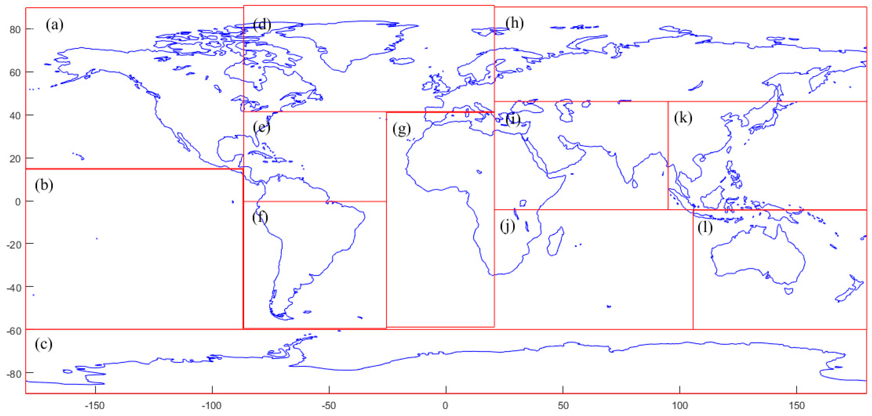
The prior knowledge of the SCTV features in the global domain, namely the geographical knowledge of SCTV distribution, is generally known according to historical experiences, which could be used to guide the sub-domain division effectively [27]. According to aircraft traffic distribution which is dense in population agglomeration while scarce in ocean regions, the global earth surface domain is split into 12 sub-domains: (a) North America; (b) Pacific Ocean; (c) Antarctica; (d) Western Europe; (e) Caribbean Sea; (f) South America; (g) Atlantic and Western Africa; (h) Russia; (i) Middle East; (j) Indian Ocean; (k) East Asia; (l) Oceania, as shown in Figure 3 (the global coastline is drawn in MATLAB (MathWorks, Natick, MA, USA)). Furthermore, (b) the Pacific Ocean, (c) Antarctica, (g) Atlantic and Western Africa and (j) Indian Ocean have scarce traffic distribution due to the large marine area. Hence, the satellite payload could be kept at low power or shut down at these sub-domains, and there is no need to construct the surrogate in these areas. For the other eight regions, the onboard resources need be allocated dynamically, and in this paper surrogates are built for these eight regions. Notice that for different satellite missions, the geographical distribution variances of SCTV present different characteristics. Thus, the division of the global earth surface domain with prior knowledge should be based on the specific mission background. For example, ship traffic distribution is dense in vast ocean regions while aircraft traffic distribution is scarce in those areas, and therefore the focus of the division should be different for these two missions. In this paper, surrogate modeling for air traffic SCTV prediction is studied for illustration.
Due to the geographical distribution variances of SCTV, there are distinct SCTV features in each sub-domain. To enhance the surrogate accuracy in each sub-domain, the ensemble modeling method is an effective way [18]. The commonly used approach is the weighted aggregation method described in Section 2.4. However, when forming a weighted ensemble by (13) the weighted sum of all the candidate surrogates, it is possible that the inaccurate surrogate is included which will lead to loss of accuracy. Based on this consideration, instead of employing all the candidate surrogates, in this paper it is proposed to only select a part of them as contributing models with high accuracy to constitute the ensemble, which is named partial weighted aggregation method (PWTA). The details of PWTA are as follows.
First, for the k th sub-domain, construct multiple different candidate surrogates, and calculate the corresponding GMSE based on leave-one-out cross-validation by (15) of each surrogate as the criterion to measure its accuracy. Then the sequence of the surrogates according to GMSE in the ascending order can be obtained, and denote the candidate model set with the ranking sequence as { M ( i ) k } i = 1 , 2 , , n M with the corresponding GMSE and predictor sets denoted as { GMSE ( i ) k } i = 1 , 2 , , n M and { y ^ ( i ) k } i = 1 , 2 , , n M . Here, n M is the total number of the candidate surrogates. To choose the relatively more accurate surrogates from the candidate set { M ( i ) k } i = 1 , 2 , , n M so as to compose a more accurate ensemble, the first issue is to define the number of contributing surrogates n M k * n M to be selected. There are two important points that should be taken into consideration during setting the threshold for the “more accurate” candidate selection. On one hand, because each domain has distinct SCTV features and different surrogates have different performance, the threshold is preferred to be decided adaptively in each sub-domain rather than simply fixed by a specific number or ratio. On the other hand, considering that GMSE values of the inaccurate surrogates might greatly deviate from those of the accurate surrogates, the threshold could be determined by borrowing the idea of identifying the outliers [28] so as to rationally screen out the surrogates with low accuracy (or comparatively large GMSE values). According to these considerations, the number of contributing surrogates n M k * to be selected in the k th sub-domain is set as
GMSE ( n M k * ) k t k + δ C k GMSE ( n M k * + 1 ) k > t k + δ C k ,
where δ + is a user-defined control parameter. From our numerical experience, it is appropriate to take 1 to 3 for δ . When the value of δ is small, there may be less candidate surrogates chosen as positively contributing models. With the enlarged δ value, it is likely to select more candidate surrogates into the ultimate ensemble. t k and C k are the mean and standard deviation of the GMSE set in the k th sub-domain. To eliminate the negative effect of the inaccurate models GMSE so as to obtain a robust estimation, t k and C k are solved using the first M = [ 3 n M / 4 ] ( [ · ] denotes the rounding operation) elements of the set { GMSE ( i ) k } i = 1 , 2 , , n M [29]
t k = 1 M i = 1 M GMSE ( i ) k C k = 1 M i = 1 M ( GMSE ( i ) k t k ) 2 .
From Equations (19) and (20) it can be observed that for different sub-domains, there may be different types as well as different numbers of the contributing surrogates. To combine the independent contributing models into the ultimate ensemble for each sub-domain SCTV prediction, the associated weights are calculated for the k th sub-domain by
w ( i ) k = j = 1 , j i n M k * GMSE ( j ) k ( n M k * 1 ) j = 1 n M k * GMSE ( j ) k , i = 1 , , n M k * ,
and the prediction value of the ensemble in the k th sub-domain is
y ^ P W T A k = i = 1 n M k * w ( i ) k y ^ ( i ) k .
After the surrogate ensemble modeling procedure, eight ensembles are obtained for the eight sub-domains. Notice that for points at the boundary of the sub-domains which belong to two or more sub-domains at the same time, their SCTV values are determined by averaging the predictions of the ensembles from the sub-domains sharing these boundaries.

4. Experimental Results

4.1. Experimental Setting

To testify the proposed PWTA method for the SCTV prediction, it is compared with the following surrogate models: (1) Polynomial Response Surface (PRS), (2) Ordinary Kriging (OK), (3) Radial Basis Function (RBF), (4) Weighted aggregation method (WTA) and (5) BestGMSE surrogate, which are introduced in Section 2. DACE toolbox of MATLAB is used to construct the OK model [30]. The parameter settings are presented in Table 1. The following metrics are used to evaluate the predictive capabilities of the surrogate models in the sub-domains.
●  R square ( R 2 ) correlation coefficient
The R k 2 correlation coefficient of the model in the k th ( k = 1 , 2 , , 8 ) sub-domain is represented as
R k 2 = 1 l = 1 N t k ( y k ( l ) y ^ ( x k ( l ) ) ) 2 l = 1 N t k ( y k ( l ) y ¯ k ) 2 ,
where N t k is the number of test points in the k th sub-domain. y k ( l ) and y ^ ( x k ( l ) ) denotes the actual response and the predicted response at the l th test point of the k th sub-domain respectively, and y ¯ k is the actual averaged response of the test set in the k th sub-domain.
● Normalized root mean squared error (NRMSE)
The NRMSE k of the model in the k th sub-domain is given by
NRMSE k = l = 1 N t k ( y k ( l ) y ^ ( x k ( l ) ) ) 2 l = 1 N t k ( y k ( l ) ) 2 ,
● Normalized maximum absolute error (NMAE)
The NMAE k of the model in the k th sub-domain is calculated by
NMAE k = max ( | y k ( 1 ) y ^ ( x k ( 1 ) ) | , , | y k ( N t k ) y ^ ( x k ( N t k ) ) | ) 2 1 N t k l = 1 N t k ( y k ( l ) ) 2 .
In this paper, the air traffic SCTV data downloaded from TianTuo-3 is processed by MATLAB and used to perform experiments. Test points are sampled every two longitudes as well as every two latitudes, and the number of the sampled points for each sub-domain is shown in Table 2. In addition to investigate the SCTV prediction capability in each sub-domain, to further verify the surrogate robustness in the global domain, in this paper the R 2 correlation coefficient, NRMSE, and NMAE of the model in the global domain, denoted as R g 2 , NRMSE g and NMAE g , are also investigated, which are
R g 2 = 1 k = 1 8 l = 1 N t k ( y k ( l ) y ^ ( x k ( l ) ) ) 2 k = 1 8 l = 1 N t k ( y k ( l ) y ¯ k ) 2 NRMSE g = k = 1 8 l = 1 N t k ( y k ( l ) y ^ ( x k ( l ) ) ) 2 k = 1 8 l = 1 N t k ( y k ( l ) ) 2 NMAE g = max ( | y 1 ( 1 ) y ^ ( x 1 ( 1 ) ) | , , | y 8 ( N t 8 ) y ^ ( x 8 ( N t 8 ) ) | ) 2 1 8 k = 1 8 ( 1 N t k l = 1 N t k ( y k ( l ) ) 2 ) .
For the high-quality surrogate model, the R 2 correlation coefficient should be close to 1, while NRMSE and NMAE should be low.

4.2. Effect of Design of Experiment for Training Sample Generation

The training points for surrogate modeling are typically generated by design of experiments (DOE). A commonly used DOE method is Latin hypercube sampling (LHS) which has proved conducive to improving the quality of approximation for its uniform sampling performance and scalability for high-dimensional problems [31]. However, a major disadvantage of LHS is randomness in sampling, which has great effect on sample quality. In this SCTV prediction problem with only two-dimensional geographical input, full-factorial design (FFD) [31] can be applied to ensure the uniform design of experiment. To demonstrate the effect of DOE on the proposed PWTA method and the candidate surrogates, 60 training points are sampled in each sub-domain using LHS and FFD respectively, and PRS, OK, RBF as well as PWTA are used to construct the surrogates for each sub-domain based on those training sets. Due to the randomness of LHS, the mean R 2 values obtained by 100 independent runs are used for comparison. The results are presented in Table 3. The best value in each column is shown in bold for ease of comparison. It can be observed that OK, RBF, and PWTA using FFD generally perform better than those using LHS. It suggests that FFD can improve the prediction accuracy of the models in this two-dimensional SCTV prediction problem. Furthermore, for these two different DOE methods, PWTA performs well both in sub-domains and globally. The accuracy issue will be further discussed in Section 4.5.

4.3. Effect of the Training Sample Size

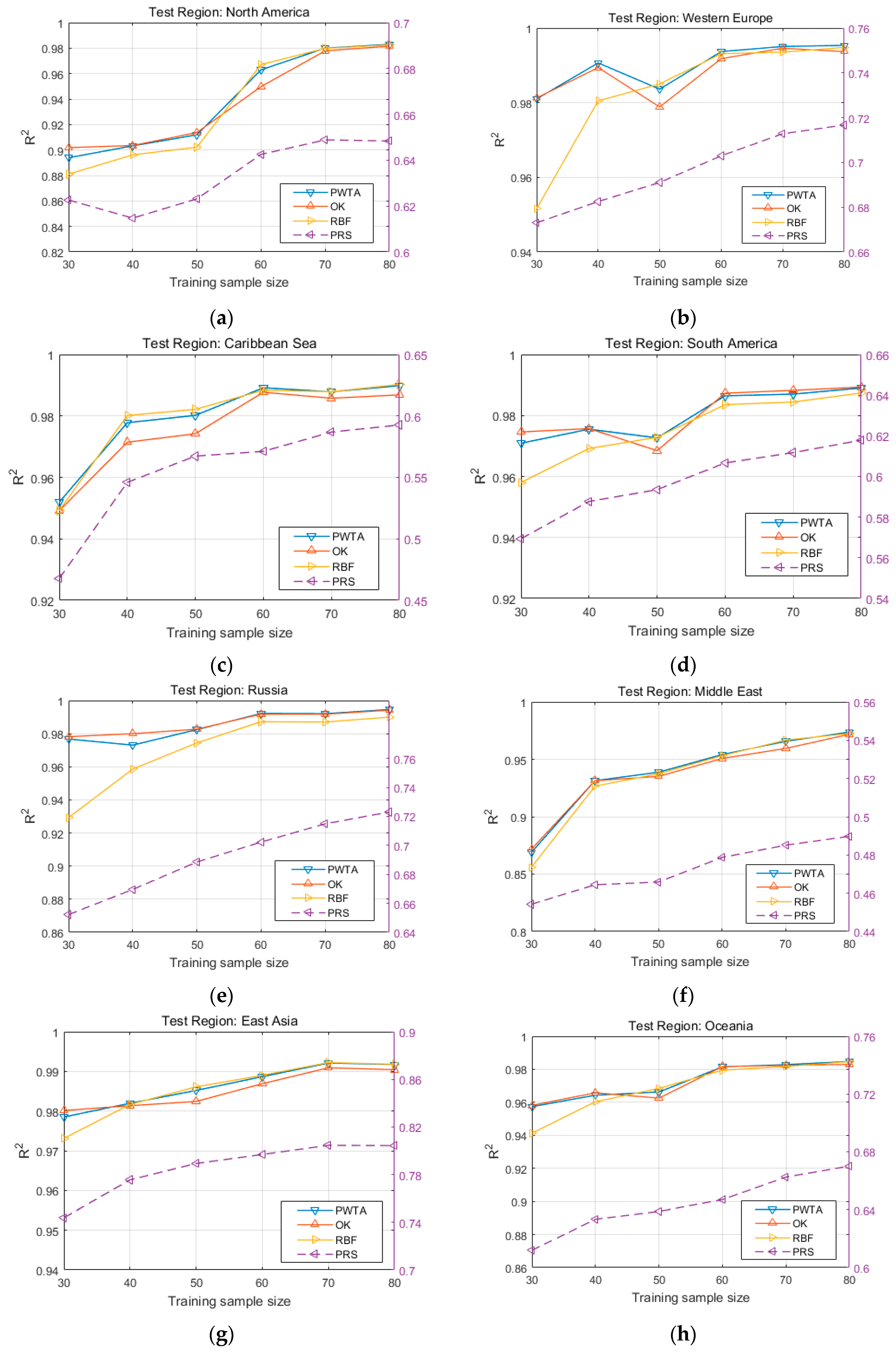
To investigate the effect of the training sample size on the proposed PWTA method and the candidate surrogates, 30, 40, 50, 60, 70, and 80 training points are sampled in each sub-domain respectively using full-factorial design. PRS, OK, RBF, and PWTA are constructed for each sub-domain with those training sets, respectively. From the experiments we observed that when training points are less than 30, PWTA is less accurate for most sub-domains. With more than 80 training points, the accuracy of PWTA becomes stable and cannot be improved obviously. Thus, the range between 30 to 80 training points is selected to better show the growth trends of model accuracy. Figure 4 presents R 2 of different surrogates vary with the training sample size in the eight sub-domains. The R 2 values of the different models in the global domain are shown in Table 4. The best value in each column is shown in bold for ease of comparison. From Figure 4, it can be easily seen that PRS performs poorly for the eight sub-domains. When the training sample size is small, R 2 of RBF are greatly lower than those of OK. With the enlarged training sample size, OK performs poorer than RBF for North America, Western Europe, East Asia, and Caribbean Sea regions, while for Russia and South America regions, the accuracy of OK are better. It suggests that the performances of different surrogates vary greatly in different sub-domains with different training sample sizes. However, for PWTA, it can be observed that for all the sub-domains and for all the different training sample number conditions, PWTA can perform robustly with top one or two accuracy level. In Table 4, the results show that with small training sample sizes, PWTA performs secondary but comparably well to OK (with less than 0.177% relative difference) which has the highest accuracy in terms of R 2 in global domain. When the number of training points is greater than 40, PWTA universally outperforms the other surrogates. This indicates that for different sub-domains as well as different training sample sizes, PWTA is a more robust choice. Furthermore, it also can be observed that the overall performance of all the surrogates become better and better as the training sample size increases. However, after 60 training points the trends of growth become smaller. Thus, the numbers of the training sample points are set to 60 in the eight sub-domains for the subsequent experiments.

4.4. Effect of the Sub-Domain Division

To demonstrate the effect of the sub-domain division step for SCTV surrogate modeling, the proposed PWTA method is used to build the surrogates for each sub-domain after domain division based on the knowledge of geographical SCTV distribution (denoted as PWTASD) and also used to directly build a surrogate for the global domain (denoted as PWTAGD). For PWTASD, 60 training points are sampled in each sub-domain using full-factorial design. For PWTAGD, all the samples obtained in PWTASD are used for the global surrogate modeling. Table 5 presents the R 2 correlation coefficients, NRMSE and NMAE metrics of PWTASD and PWTAGD in each sub-domain, as well as the summary values in the global domain. The best value in each column is shown in bold for ease of comparison. From Table 5, it can be seen that PWTASD performs better than PWTAGD in the eight sub-domains and across the entire domain. It clearly validates the effect of the sub-domain division of the proposed method which can better capture the regional SCTV features by building the independent ensemble for each sub-domain, leading to better approximation quality.

4.5. Accuracy and Robustness

The accuracy and robustness of different surrogates (obtained with 60 training points) are evaluated by R 2 and NRMSE in each sub-domain as well as globally, as shown in Table 6. The best value in each column is shown in bold for ease of comparison. The results show that in the global domain the overall accuracy of PWTA is better than that of the other surrogates. Moreover, PWTA also outperforms the other surrogates for most sub-domains, except North America, South America, East Asia, and Oceania areas. Although PWTA is not the best for those sub-domains, it performs comparably well (rank second in terms of accuracy) to the best model in these sub-domains (with less than 0.06% relative difference). It suggests that PWTA performs robustly well in this SCTV prediction problem. For the BestGMSE surrogate, it can be seen that its overall performance is poorer than that of PWTA. Especially in South America and Russia areas, the accuracy of the BestGMSE surrogate is the same as that of RBF, i.e., RBF is chosen as the “optimal model” based on the criterion of GMSE which only considers training points. However, OK that has better performance on the test set is neglected. This indicates that for the BestGMSE surrogate there is indeed a risk of selecting the suboptimal model which lacks good generalization capability. However, for PWTA, this risk could be effectively avoided by the ensemble modeling. Moreover, it can be also observed that WTA has poorer performance compared to PWTA, which confirms that adding the inaccurate surrogates into the ultimate ensemble would result in loss of accuracy.
In summary, compared with surrogate ensemble modeling globally, the proposed sub-domain modeling method has better accuracy and robustness. Moreover, the overall performance of PWTA which adaptively selects contributing surrogates for different sub-domains is better than not only the candidate surrogates but also the other two surrogate ensemble modeling methods (WTA and BestGMSE). These suggest that the method proposed in this paper can better capture the local characteristics of the objective function in each sub-domain with different SCTV features.

5. Conclusions

In this paper, an enhanced surrogate ensemble modeling method is proposed for the SCTV prediction. Unlike traditional onboard SCTV prediction by the data table lookup, this paper proposes to distill the data into a surrogate model to be uploaded to a satellite, which can both save the valuable communication link resource and improve the SCTV prediction accuracy compared to table lookup. The proposed surrogate ensemble modeling method first divides the global earth surface space into multiple sub-domains according to the prior geographical knowledge of the SCTV distribution, and then constructs multiple candidate surrogates in each sub-domain. To fully exploit the candidate surrogates and combine them into a more accurate ensemble, a partial weighted aggregation method (PWTA) is developed. For each sub-domain, PWTA adaptively selects the candidate surrogates with higher accuracy as the contributing models, based on which the ultimate ensemble is constructed for each sub-domain SCTV prediction. The proposed surrogate ensemble modeling method could obtain the independent contributing surrogates and weights for each sub-domain so that the ensembles are more suitable for the corresponding sub-domains. Thus, the prediction accuracy and robustness of the ensembles can be improved in the corresponding sub-domains and across the entire domain, which is verified in the test section. For future works, we would like to further study the proposed surrogate ensemble modeling method on a more diverse set of test problems, and more kinds of candidate surrogates will be considered. Moreover, the surrogate update method with the dynamically accumulated SCTV data will be researched to further improve the surrogate prediction accuracy and modeling efficiency.

Author Contributions

S.Y., Y.Z. and W.Y. conceived the PWTA method and designed the experiments; S.Y. performed the experiments and analyzed the data; Q.C. and X.C. contributed reagents/materials/analysis tools; S.Y. wrote the paper under the supervision of Y.Z. and W.Y.

Funding

This work was supported in part by National Natural Science Foundation of China under Grant No.51675525 and 11725211.

Conflicts of Interest

The authors declare that the grant, scholarship, and/or funding mentioned in the Acknowledge section do not lead to any conflict of interest. Additionally, the authors declare that there is no conflict of interest regarding the publication of this manuscript.

References

  1. Bettray, A.; Litschke, O.; Baggen, L. Multi-beam antenna for space-based ADS-B. In Proceedings of the 2013 IEEE International Symposium on Phased Array Systems and Technology, Waltham, MA, USA, 15–18 October 2013; pp. 227–231. [Google Scholar]
  2. Fournier, M.; Casey Hilliard, R.; Rezaee, S. Past, present, and future of the satellite-based automatic identification system: Areas of applications (2004–2016). WMU J. Marit. Aff. 2018, 17, 311–345. [Google Scholar] [CrossRef]
  3. He, Y.; Jia, Y.; Zhong, X. A traffic-awareness dynamic resource allocation scheme based on multi-objective optimization in multi-beam mobile satellite communication systems. Int. J. Distrib. Sens. Netw. 2017, 13, 1–14. [Google Scholar] [CrossRef]
  4. Yu, S.; Chen, L.; Li, S.; Zhang, X. Adaptive Multi-beamforming for Space-based ADS-B. J. Navig. 2018, 72, 359–374. [Google Scholar] [CrossRef]
  5. Goel, T.; Hafkta, R.T.; Shyy, W. Comparing error estimation measures for polynomial and kriging approximation of noise-free functions. Struct. Multidiscip. Optim. 2008, 38, 429–442. [Google Scholar] [CrossRef]
  6. Clark, D.L.; Bae, H.-R.; Gobal, K.; Penmetsa, R. Engineering Design Exploration Using Locally Optimized Covariance Kriging. AIAA J. 2016, 54, 3160–3175. [Google Scholar] [CrossRef]
  7. Sun, Z.; Zhang, Y.; Yang, G. Surrogate Based Optimization of Aerodynamic Noise for Streamlined Shape of High Speed Trains. Appl. Sci. 2017, 7, 196. [Google Scholar] [CrossRef]
  8. Yao, W.; Chen, X.; Zhao, Y. Concurrent subspace width optimization method for RBF neural network modeling. IEEE Trans. Neural Netw Learn. Syst 2012, 23, 247–259. [Google Scholar]
  9. Clarke, S.M.; Simpson, T.W. Analysis of Support Vector Regression for Approximation of Complex Engineering Analyses. J. Mech. Des. 2005, 127, 77–87. [Google Scholar] [CrossRef]
  10. Sun, G.; Song, X.G.; Baek, S.; Li, G. Crashworthiness optimization of foam-filled tapered thin-walled structure using multiple surrogate models. Struct. Multidiscip. Optim. 2013, 47, 221–231. [Google Scholar]
  11. Forrester, I.J.; Keane, A.J. Recent advances in surrogate-based optimization. Prog. Aerosp. Sci. 2009, 45, 50–79. [Google Scholar] [CrossRef]
  12. Bhosekar, A.; Ierapetritou, M. Advances in surrogate based modeling, feasibility analysis, and optimization: A review. Comput. Chem. Eng. 2018, 108, 250–267. [Google Scholar] [CrossRef]
  13. Wang, G.; Shan, S. Review of Metamodeling Techniques in Support of Engineering Design Optimization. ASME J. Mech Des. 2007, 129, 370–380. [Google Scholar] [CrossRef]
  14. Goel, T.; Haftka, R.T.; Shyy, W.; Queipo, N.V. Ensemble of surrogates. Struct. Multidiscip. Optim. 2006, 33, 199–216. [Google Scholar] [CrossRef]
  15. Glaz, B.; Goel, T.; Liu, L.; Friedmann, P.; Haftka, R.T. Application of a Weighted Average Surrogate Approach to Helicopter Rotor Blade Vibration Reduction. In Proceedings of the 48th AIAA/AMSE/AHS/ASC Structures, Structural Dynamic, and Materials Conference, Waikiki, HI, USA, 23–26 April 2007; pp. 1–25. [Google Scholar]
  16. Wang, H.; Doherty, J. Committee-Based Active Learning for Surrogate-Assisted Particle Swarm Optimization of Expensive Problems. IEEE Trans. Cybern. 2017, 47, 2664–2677. [Google Scholar] [CrossRef] [Green Version]
  17. Gu, X.; Wang, H. Reliability-based design optimization for vehicle occupant protection system based on ensemble of metamodels. Struct. Multidiscip. Optim. 2015, 51, 533–546. [Google Scholar] [CrossRef]
  18. Viana, F.; Steffen, V. Multiple surrogates: How cross-validation errors can help us to obtain the best predictor. Struct. Multidiscip. Optim. 2009, 39, 439–457. [Google Scholar] [CrossRef]
  19. Acar, E. Various approaches for constructing an ensemble of metamodels using local measures. Struct. Multidiscip. Optim. 2010, 42, 879–896. [Google Scholar] [CrossRef]
  20. Zhang, J.; Chowdhury, S.; Messac, A. An adaptive hybrid surrogate model. Struct. Multidiscip. Optim. 2012, 46, 223–238. [Google Scholar] [CrossRef]
  21. Yin, H.; Fang, H.; Wen, G.; Gutowski, M.; Xiao, Y. On the ensemble of metamodels with multiple regional optimized weight factors. Struct. Multidiscip. Optim. 2018, 58, 245–263. [Google Scholar] [CrossRef]
  22. Lee, Y.; Choi, D.H. Pointwise ensemble of meta-models using v nearest points cross-validation. Struct. Multidiscip. Optim. 2014, 50, 383–394. [Google Scholar] [CrossRef]
  23. Zhou, Z.; Wu, J.; Tang, W. Ensembling Neural Networks: Many Could Be Better Than All. Artif. Intell. 2002, 137, 239–263. [Google Scholar] [CrossRef]
  24. Zhang, Y.; Yao, W.; Ye, S.; Chen, X. A regularization method for constructing trend function in Kriging model. Struct. Multidiscip. Optim. 2018, 59, 1221–1239. [Google Scholar] [CrossRef]
  25. Qian, C.; Zhang, S.; Zhou, W. Traffic-based dynamic beam coverage adjustment in satellite mobile communication. In Proceedings of the Sixth International Conference on Wireless Communications & Signal Processing, Hefei, China, 23–25 October 2014; pp. 1–6. [Google Scholar]
  26. Li, S.; Chen, X.; Chen, L.; Zhao, Y.; Sheng, T.; Bai, Y. Data Reception Analysis of the AIS on board the TianTuo-3 Satellite. J. Navig. 2017, 70, 761–774. [Google Scholar] [CrossRef]
  27. Machado, A.; Gee, J.; Campos, M. Substructural segmentation based on regional shape differences. In Proceedings of the XV Brazilian Symposium on Computer Graphics and Image Processing, Fortaleze, CE, Brazil, 7–10 October 2002; pp. 3–10. [Google Scholar]
  28. Li, L.; Wen, Z.; Wang, Z. Outlier Detection and Correction During the Process of Groundwater Lever Monitoring Base on Pauta Criterion with Self-learning and Smooth Processing. In Theory, Methodology, Tools and Applications for Modeling and Simulation of Complex Systems: 16th Asia Simulation Conference and SCS Autumn Simulation Multi-Conference, AsiaSim/SCS AutumnSim 2016, Beijing, China, 8–11 October 2016; Springer: Singapore, 2016; pp. 497–503. [Google Scholar]
  29. Filzmoser, P.; Garrett, R.G.; Reimann, C. Multivariate outlier detection in exploration geochemistry. Comput. Geosci. 2005, 31, 579–587. [Google Scholar] [CrossRef]
  30. Lophaven, S.N.; Nielsen, H.B.; Søndergaard, J. Aspect of the Matlab Toolbox DACE; Report IMM-TR-2002-13; Informatics and Mathematical Modelling; DTU: Kongens Lyngby, Denmark, 2002. [Google Scholar]
  31. Forrester, I.J.; Sóbester, A.; Keane, A.J. Engineering Design via Surrogate Modelling: A Practical Guide; John Weily&Sons: Hoboken, NJ, USA, 2008. [Google Scholar]
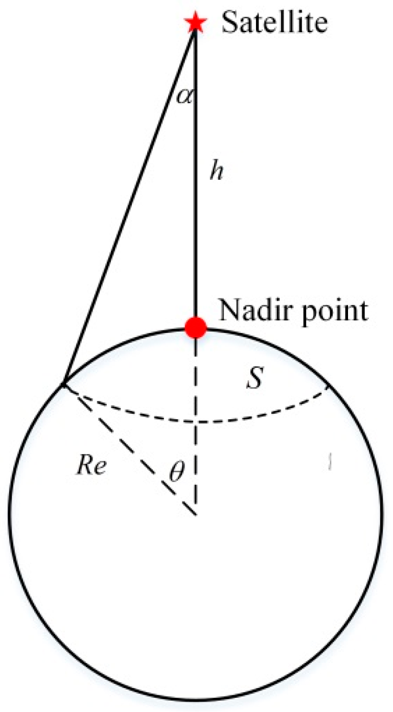
Figure 1. Diagram of the coverage region on the earth’s surface.
Applsci 09 03689 g001
Figure 2. Aircraft traffic density distribution.
Applsci 09 03689 g002
Figure 3. Division of the global earth surface domain for air traffic distribution. (a) North America; (b) Pacific Ocean; (c) Antarctica; (d) Western Europe; (e) Caribbean Sea; (f) South America; (g) Atlantic and Western Africa; (h) Russia; (i) Middle East; (j) Indian Ocean; (k) East Asia; (l) Oceania.
Applsci 09 03689 g003
Figure 4. R 2 varying with training sample size of different surrogates in (a) North America, (b) Western Europe, (c) Caribbean Sea, (d) South America, (e) Russia, (f) Middle East, (g) East Asia and (h) Oceania. For clarity, R 2 of the PRS surrogate are indicated by the dashed purple line with the purple y-axis on the right, and the others are presented by the solid line with the black y-axis on the left.
Applsci 09 03689 g004
Table 1. Parameters for different surrogate models.
Surrogate ModelDetails
PRSThe second-order polynomials are used
OKA constant regression function and a Gaussian correlation model are employed in the mode. In all cases, θ 0 = 1 m × 1 , and 1 θ i 5 , for i = 1 , 2 , , m where m is the number of variables and 1 m × 1 is the vector whose entries are all equal to 1
RBFThe form of basis function is the multiquadric function and we set c = 0.9 [20]
PWTAThe above three models are used as the candidate surrogates. The control parameter δ = 3
WTAThe same as PWTA
BestGMSE surrogateThe same as PWTA
Table 2. Numerical setup for the sub-domains.
Sub-DomainsNo. of Test Sample Points
North America1680
Western Europe1370
Caribbean Sea695
South America1045
Russia1790
Middle East930
East Asia1060
Oceania1025
Table 3. Comparisons of R 2 for different surrogates using LHS and FFD, respectively.
Performance MetricSurrogate ModelNorth AmericaWestern EuropeCaribbean SeaSouth AmericaRussiaMiddle EastEast AsiaOce-aniaGlobal Domain
R 2 of the models using FFDPRS0.64250.70290.57120.60670.70230.47870.79680.64690.6760
OK0.96220.99180.98770.98730.99180.95070.98690.98160.9837
RBF0.96710.99310.98840.98360.98720.95320.98900.97950.9830
PWTA0.96670.99370.98920.98660.99200.95410.98850.98140.9846
Mean R 2 of the models using LHSPRS0.62660.73940.55910.64260.73070.45340.82540.71410.7021
OK0.91110.96350.91700.93420.94390.85220.95000.92590.9332
RBF0.92250.95820.93760.95210.95070.92140.98250.95940.9564
PWTA0.93240.97350.93890.95450.96750.91070.97980.95790.9593
Table 4. Comparisons of R 2 for different surrogates in the global domain under different training sample sizes.
Surrogate Model30 Training Points in Each Sub-Domain40 Training Points in Each Sub-Domain50 Training Points in Each Sub-Domain60 Training Points in Each Sub-Domain70 Training Points in Each Sub-Domain80 Training Points in Each Sub-Domain
PRS0.63330.65570.66580.67600.68550.6901
OK0.96130.97030.96940.98310.98620.9880
RBF0.94280.96450.97130.98300.98580.9880
PWTA0.95960.96970.97220.98450.98720.9891
Table 5. Comparisons of R 2 , NRMSE, and NMAE for PWTASD and PWTAGD.
Performance MetricSurrogate ModelNorth AmericaWestern EuropeCaribbean SeaSouth AmericaRussiaMiddle EastEast AsiaOce-aniaGlobal Domain
R 2 PWTASD0.9670.9940.9890.9870.9920.9540.9890.9810.985
PWTAGD0.9600.9920.9860.9780.9850.9460.9870.9700.980
NRMSEPWTASD0.0820.0370.0500.0810.0530.0770.0590.0820.069
PWTAGD0.0900.0430.0570.1040.0720.0840.0630.1040.079
NMAEPWTASD0.4250.1550.1660.3720.2290.2820.2840.4180.447
PWTAGD0.4260.1680.2130.3770.3060.2840.2860.5130.549
Table 6. Comparisons of R 2 and NRMSE for different surrogates.
Performance MetricSurrogate ModelNorth AmericaWestern EuropeCaribbean SeaSouth AmericaRussiaMiddle EastEast AsiaOceaniaGlobal Domain
R 2 PRS0.64250.70290.57120.60670.70230.47870.79680.64690.6760
OK0.96220.99180.98770.98730.99180.95070.98690.98160.9837
RBF0.96710.99310.98840.98360.98720.95320.98900.97950.9830
PWTA0.96670.99370.98920.98660.99200.95410.98850.98140.9846
WTA0.94700.96880.96120.95840.97290.91840.97710.95560.9626
BestGMSE0.96710.99310.98840.98360.98720.95320.98900.98160.9833
NRMSEPRS0.27000.25480.31310.43780.32450.26020.25150.35930.3169
OK0.08780.04230.05300.07860.05390.08000.06390.08190.0711
RBF0.08190.03880.05150.08950.06730.07790.05850.08670.0727
PWTA0.08240.03720.04960.08080.05320.07720.05980.08240.0691
WTA0.10390.08250.09420.14240.09780.10290.08440.12740.1076
BestGMSE0.08190.03880.05150.08950.06730.07790.05850.08190.0719