1. Introduction
Managed aquifer recharge (MAR) is a water resources management approach used to mitigate the negative effects of overexploitation and climate change on groundwater resources and quality. It is further utilized to balance the temporal or local water demand and availability [
1,
2]. It comprises the intended recharge of a groundwater body under controlled conditions [
3]. MAR generally involves large-scale facilities, such as injection wells, infiltration basins, or recharge dams [
4]. The construction of MAR facilities requires comprehensive planning to understand the local hydrogeological conditions, to achieve sustainable and controllable conditions, to reduce construction and maintenance costs, and to minimize the facility failure potential.
Before building MAR facilities, planning is often accompanied by field and laboratory investigations. Pilot sites and preliminary studies are required by some MAR guidelines [
5,
6]. Incorporating physical models helps to assess and define the requirements and constraints of applying MAR at a certain site. Further, the are also useful for optimizing the actual MAR site in terms of dimensions, monitoring, and operational parameters. Most commonly, surface infiltration experiments are used to understand the processes governing recharge into the unsaturated soil zone [
7,
8,
9,
10,
11]. However, laboratory and field experiments for direct infiltration into the aquifer, e.g., through aquifer storage and recovery (ASR) wells, have been conducted as well [
12,
13,
14].
The experimental design is conceptualized at different spatial scales. Usually laboratory experiments are preferred as field tests are time-consuming and costly [
12] and are often impractical for detailed process assessment [
15]. Another positive aspect of laboratory studies is that they can be conducted under adaptable and controllable boundary conditions [
7,
13,
16,
17]. However, simplifications and scale-related limitations of small-scale experiments may lead to over- or underestimation of infiltration processes [
8]. The extrapolation of results from controlled laboratory investigations to the field scale is highly uninvestigated in the context of MAR [
7] and limitations of transferring results from laboratory experiments to the field are rarely discussed [
9,
15].
These limitations can be linked to the shortcomings of laboratory experiments. Some issues, such as sidewall flow in laboratory columns, have been widely discussed [
18,
19,
20,
21]. Another critical design issue, which is not restricted to column studies, is the occurrence of preferential flow paths through macropores or fingering [
22,
23]. With regard to dimensionality, it has been stated that processes such as flow-bypassing can be not represented by 1D-systems [
8]. The lower boundary of laboratory models is often operated as free drainage out of system, which may lead to the development of capillary fringes and the lower part of the system becoming saturated [
20,
24]. Reproducing field climate conditions in the laboratory is restricted, even though seasonal conditions of temperature and radiation have a large impact on water flow and specifically clogging processes [
25,
26].
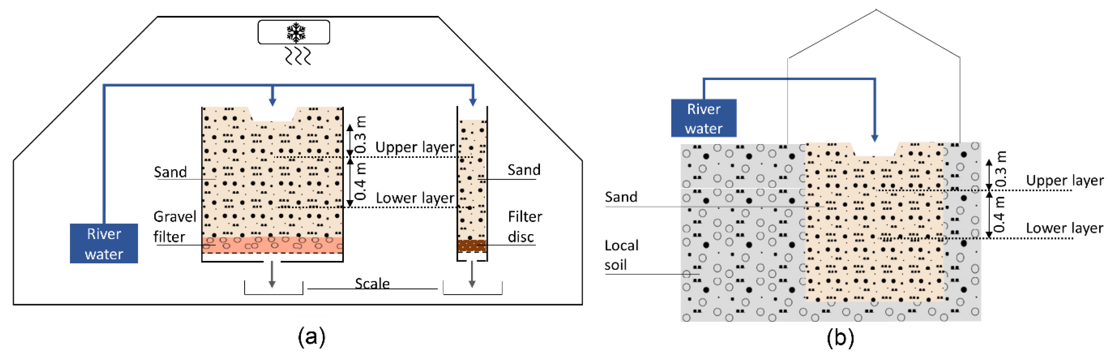
To understand the restrictions and potential of different physical models for MAR assessment, we set up surface infiltration experiments in different scales (field, laboratory) and dimensions (1D, 3D) and with several soil types but with the same operational parameters (infiltration scenarios, water quality). The results from the different setups were compared regarding the reproduction of water flow dynamics and clogging processes during intermittent infiltration experiments. The results from the statistical comparison are discussed regarding the limitations and applicability of laboratory experiments.
By increasing knowledge on their applicability in terms of MAR facility planning and by pointing out boundaries of application, their area of use can be focused to situations where laboratory experiments are actually beneficial and the results are representative of the field situation. Showing their limitations will help MAR site planners to identify areas where they must be cautious with the evaluation and application of laboratory results. Hence, this study seeks to outline the domains in which different laboratory experiments can complement MAR site planning.
3. Results
3.1. General Comparison of Experimental Data
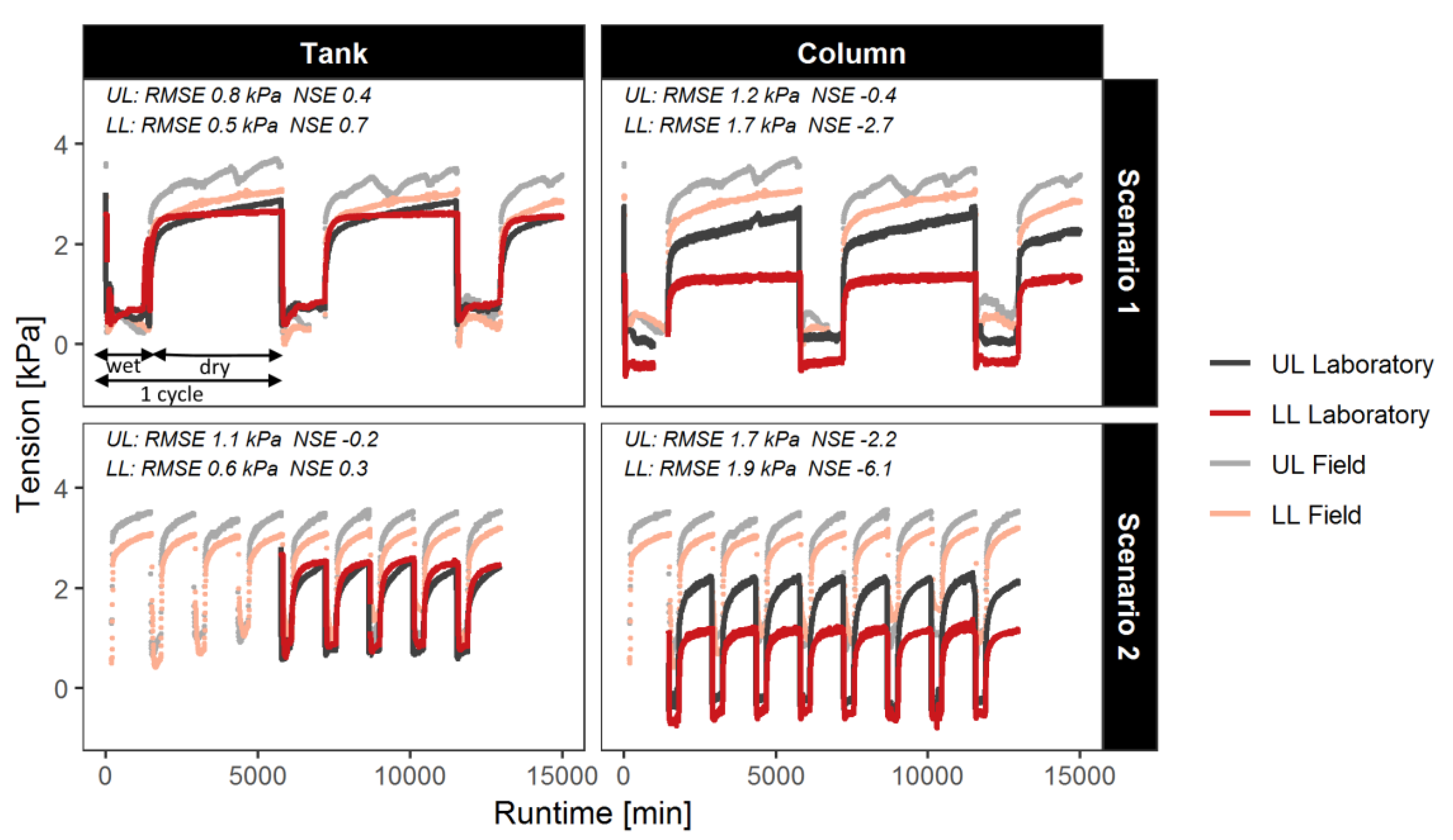
Comparing the tension measurements in the different experimental setups depicts similarities in hydraulic behavior. A relatively steady infiltration phase follows a rapid wetting phase. Drying consists of fast draining followed by a slower drainage phase (
Figure 2). Differences lie within the maximum and minimum tension values and within the increase and decrease of the slope tension. For the FIU measurements in scenario 1, an almost periodic interference can be detected, specifically during the drying phase. After analyzing the results from this scenario, the field site was covered with a roof. Scenario 2 depicts that this measure dampened the effects of rain and temperature variation as less periodic interference can be observed.
Column values always range below those of the tank and FIU values. They also show the largest difference between tension values of the upper and the lower layer. This is contrary to the tank experiment, where tension values in the upper and lower layer are similarly high. In the FIU, a small yet distinct difference between values of the upper and the lower layer can be observed.
The wetting phase of the FIU experiments can be reproduced reasonably well by the tank experiment. Here, tank and FIU values range around 0.7 kPa, whereas column values rank distinctively lower around zero kPa.
Tension values in the tank and soil column are in similar ranges during the drying phase in the upper layer, whereas FIU measurements tend to be over one kPa higher. The dry phase in the lower layer shows that, after an initial increase, values of tension are almost constant in the tank, whereas in the FIU values continue to incline. Column values of tension also stay constant during the dry phase but are almost 1.5 kPa lower than those of the other experimental units. The RMSE error always shows more than 0.4 kPa lower values for the comparison of FIU and tank than of FIU and column, indicating that the tank setup produces a more accurate representation of the FIU. The calculated NSE supports this statement, as all NSE values for the column study are below zero, demonstrating a weak representativeness of the column values for the FIU.
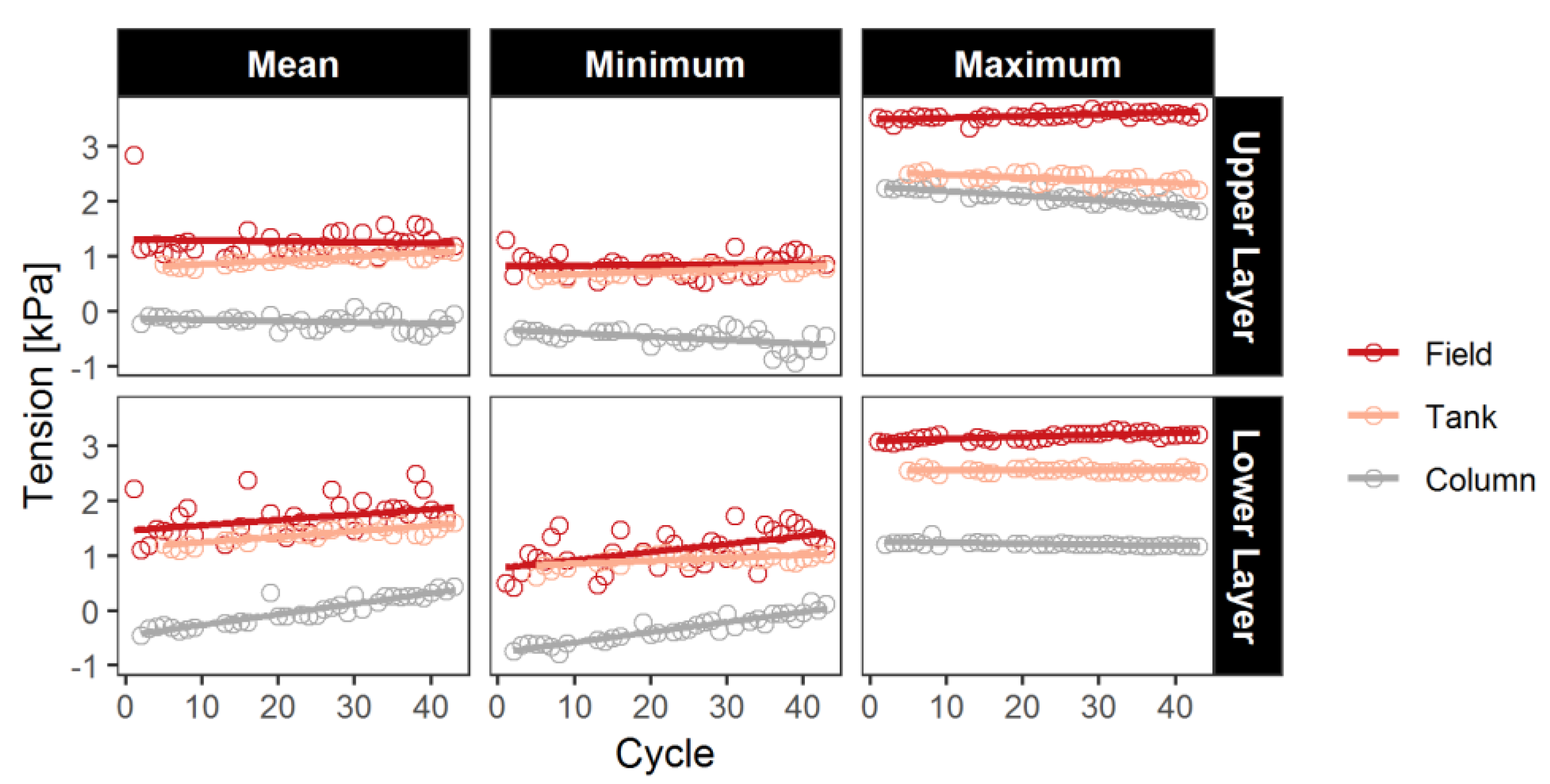
To gain further insight into the tension behavior of each experiment, mean values as well as maximum and minimum tension values were compared over the course of the experiments (
Figure 3 and
Supplementary Figure S1 for scenario 1). The results emphasize that the tank and FIU measurements were relatively close during the wetting phase, ranking around 1 kPa, and the column study produced significantly lower tension values. During the drying phase, the FIU seemed to drain stronger than the laboratory experiments.
Some of the values calculated show a distinct temporal behavior. The most significant change over time is eminent for the tension behavior in the lower layer during the wetting phase. The minimum tension values of the column increase about 1 kPa. For the other experimental setups, a less steep increase can be observed. During the drying phase, the maximum tension values stayed relatively constant over the course of the experiment for all depths and setups.
3.2. Influence of Setup Settings on Comparison
To investigate the influence of different experimental setup parameters on the results, we compared the results obtained from infiltration in different soils and under different climate conditions. The parameters used for comparison included the water content, tension, and parameters calculated from these measurements.
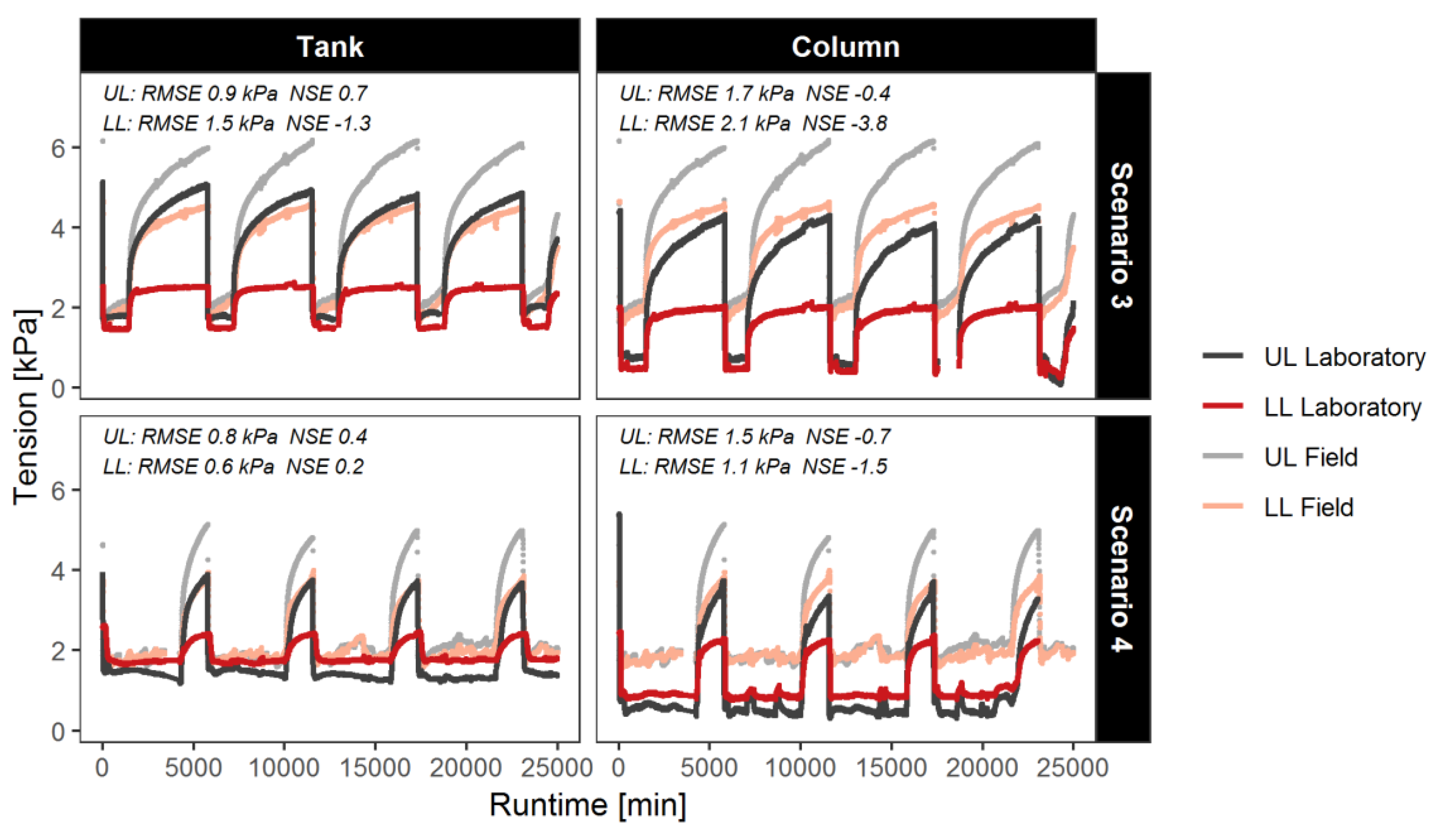
Results from infiltration scenarios with the second soil are depicted in
Figure 4. Compared to the soil discussed above, this soil was siltier. Thus, the hydraulic conductivity of soil 2 was reduced by a magnitude of 10 and led to the minimum and, especially, the maximum tension values ranking up to 2 kPa higher than the values for soil 1. It further caused a drying phase with a much clearer difference in tension behavior between the upper and the lower layer shown for all setups and scenarios. Tension in the lower layer was more than 1 kPa higher than in the upper layer, and in case of the 3-day drying phase of scenario 3, the difference became larger than 2 kPa.
Differences that have been attributed to setup modifications are also evident. Same as for soil 1, the FIU and tank values during the wetting phase were relatively close, ranking between 1.7–2 kPa. The column values were always more than 1 kPa lower during this phase, confirming the above-mentioned hypothesis. Same as above, for soil 2 the column and tank drying behavior was very similar, with a rapid drying phase in the LL followed by an almost constant tension behavior. However, column values ranked only slightly lower than tank values. Differences between laboratory and FIU values became even stronger during this phase than the ones shown in
Figure 2, with tension values up to 2 kPa lower in the FIU.
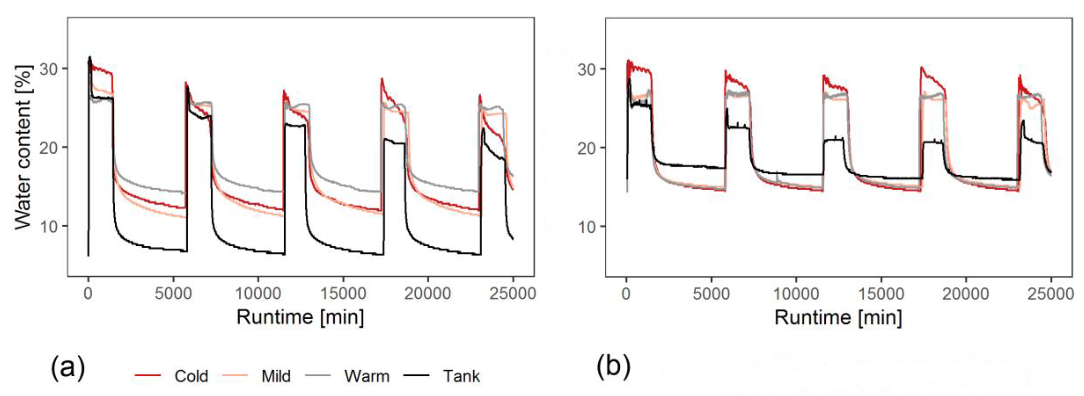
While air temperature and humidity were kept constant for the laboratory experiments, the FIU was influenced by the local climate. To assess the influence of the climate on water flow in the unsaturated zone, the experiments were repeated for three different climate scenarios (compare
Table 1, column 4–6). Results show that the difference between measurements of the FIU and tank was much larger than the difference of FIU water content measurements under different climates (
Figure 5). In the deeper layer, the influence of climate was only visible during the wet phase, where the water content measured under the cold climate was slightly higher than the water content of the experiments conducted under the other climates. The difference to the tank measurements was much more distinct, where during the wet phase water content dropped to 22%, compared to 28% in the FIU. In the lower layer, the dry phase showed no difference between field climates and the tank values are relatively close. However, draining remained relatively constant in the tank after an initial drop, whereas in the FIU a decreased but continuing draining could be observed.
In the upper layer, the influence of climate on the water content became more visible, with the drying phase showing 3% higher water content for the warm climate. Again, the difference to tank values was much more distinct with water content values during the wet phase, dropping to 22% after initially being as high as the FIU values. The largest difference could be observed during the drying phase, where values were more than 5% below those of the FIU.
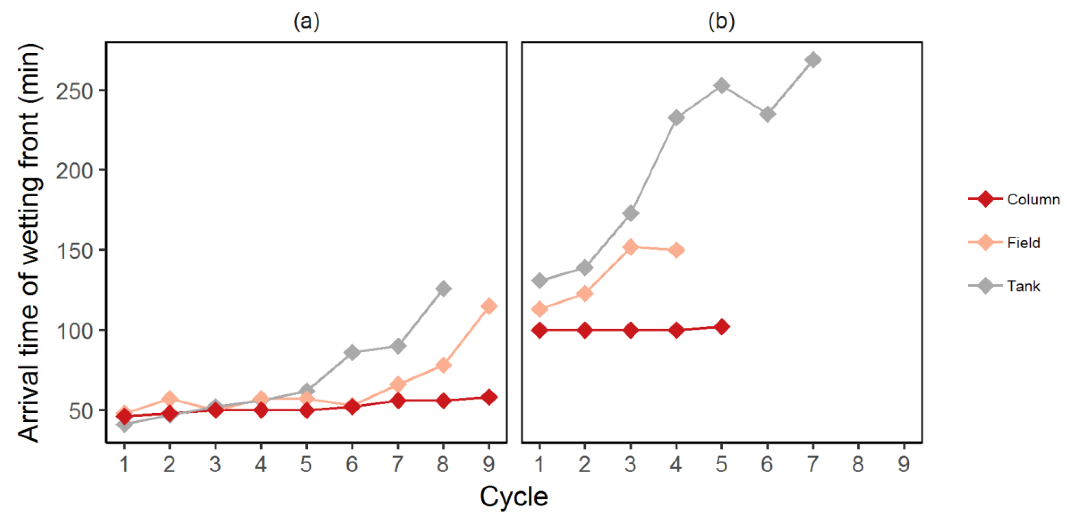
The influence of the experimental setup itself can be well observed, when assessing the arrival times of the wetting front at 0.7 m depth (
Figure 6), which was calculated as duration from infiltration start to the start of tension decrease. While in the tank and the FIU the arrival time of the wetting front increased over time by more than 100%, the arrival time in the column experiment stayed constant over time. This behavior was detected, even though all systems showed signs of clogging, with the tank and the column experiment having to be aborted due to ponding overflow.
3.3. Usability of Results for Water Flow Estimation through Laboratory Experiments
The RMSE and NSE in
Figure 2 showed that the representativeness of laboratory values for the FIU was limited. We conducted an analysis for scenario 1 for predictors that could increase the statistical representativeness looking into regression functions as well as multipliers and addends. As tension values for the wet phase are relatively constant, an addend was calculated for the difference between mean laboratory and FIU values. This value was calculated to be 0.1 kPa (upper layer) and −0.1 kPa (lower layer) for the tank values and 0.9 kPa (upper layer) and 1.4 kPa (lower layer) for the column values. These coefficients were added to all laboratory tension values of the wet phase.
For the dry phase, a regression analysis was conducted comparing different regression models (linear, quadratic, and cubic), multipliers, and addends. The linear regression model always produced the smallest RMSE. The regression function comparing upper layer tension in tank and FIU was
y = 1.6 + 0.7
x and
y = 2.1 + 0.6
x for the column and FIU, respectively. Applying the addend and regression function, the NSE was improved in both cases, for the tank from 0.8 to 0.9 and for the column from −0.4 to 0.9 (compare
Figure 2), indicating a very good match between the FIU and the adapted laboratory data. The RMSE decreased from 0.5 to 0.4 kPa for the tank experiment and from 1.2 to 0.4 kPa for the column measurement (
Supplementary Figure S2).
The regression functions and addends retrieved from analyzing scenario 1 were further used to adapt the measured laboratory data of scenario 2 to assess their representativeness for scenarios with differing boundary conditions. In this case, the climate and the length of the cycles changed (
Table 1).
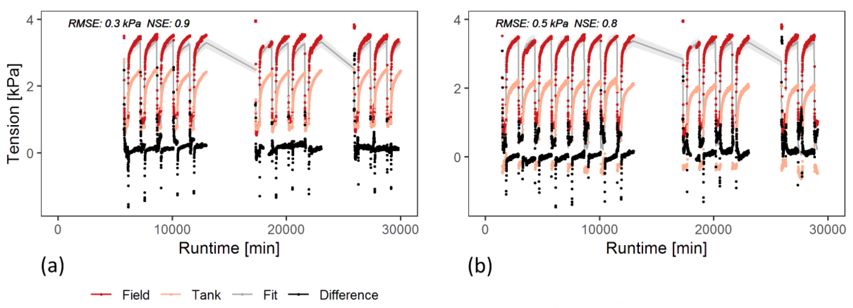
The results depicted in
Figure 7 show a good representativeness of the calculated predictors. Before, the laboratory data was visibly below the FIU measurements but through utilization of the regression function, the measurements could be well adapted to fit the FIU values. For the drying phase, most FIU values lay within the confidence interval of the laboratory values that were adapted by the predictors. The difference mapped in
Figure 7 was calculated by subtracting the FIU and the adapted laboratory tension values. For the drying phase, the difference shows values close to zero. This was also represented in the RMSE, which decreased significantly from 1.1 to 0.3 kPa (tank) and from 1.7 to 0.5 kPa (column). The biggest errors were obtained during the wetting phase and the rapid shifts from infiltration to drying and vice versa.
4. Discussion
The setup of the laboratory experiments caused distinct differences compared to the FIU measurements. Dimensionality, the lower boundary condition, sidewall flow, and climate are factors that could be identified as reasons for the differences shown by the statistical parameters.
The dimensionality of the column led to restricted lateral flow and, thus, an overall higher degree of saturation in comparison with the 3D experiments. It further stimulated the entrapment of air during intermittent infiltration, which could not escape laterally. Entrapped air can lead to reduced hydraulic conductivity and a further increased degree of saturation [
33,
34,
35]. Studies showed that this effect becomes less prominent for homogenous soils [
36], as well as for coarse soils, where air can escape upwards [
37]. Air entrapment becomes stronger the finer the soils [
37]. Thus, the higher silt content of the second soil could have increased the effect of air blockage and respective higher saturation degree. This would lead to a more distinct difference between the tension values from the laboratory experiments and the FIU.
The lower tension measurements in the deeper layers of the laboratory experiments can be attributed to the free drainage boundary condition [
20]. Water starts percolating from the drainage layer only after full saturation has been reached, leading to the build-up of a capillary fringe that can be up to 30 cm thick for sandy soils [
38]. The siltier second soil could lead to an even higher built-up of the capillary fringe [
38]. Since the measurement point in the lower layer is only 16 cm above the drainage, an influence of the capillary fringe is highly probable. The constant tension levels in the laboratory experiments further point to the restricted free outflow at the bottom. In the FIU, dewatering continues after the initial phase of rapid drainage. In the laboratory experiments, when during the drying phase no water flows in from the top layer, the degree of saturation at the bottom of the profile was insufficient to activate percolation into the drainage layer. Thus, some water remained in the lower layer of the experimental setup. This effect is amplified in the column where restricted lateral flow in combination with constrained drainage led to a significantly higher water filled pore space of the soil.
The constant arrival times of the wetting front in the column experiment could be triggered by preferential flow paths, such as sidewall flow. This effect is especially prominent in 1D-systems, where side walls are close to the measurement points and can potentially influence water flow measurements [
20,
21]. Here, flow time estimation through column studies is clearly limited, while tank studies show similarities to FIU measurements. Still, tank and FIU data differs in the intensity of flow time increase, indicating that general flow mechanisms are comparable, but a quantitative analysis cannot be made. Wall effects are also a cause for the phase changes, during wet-dry cycles, that were not exactly met by the different setups (
Figure 7). Preferential flow paths and fingering could also trigger this behavior.
The water content measurements of the tank and FIU coincide with the tension measurements in terms of temporal reaction to infiltration events and to the subsequent drying (
Figure 4 and
Figure 5). Assuming similar water retention curves for FIU and tank, the tension measurements would indicate, however, that water content in the FIU must always be below that measured in the tank. Results shown in
Figure 5 do not confirm this hypothesis. In fact, water content in the tank ranks only above FIU values during the drying phase in 0.7 m depth. This has two implications, as follows: (1) Water retention curves for the FIU and tank experiment are different even though the same soil was used and (2) the lower boundary condition in the tank enforces atypical water flow behavior, as, due to capillary fringe and air entrapment, the water content is higher than expected compared to the field measurements. The differences in soil water retention might be attributed to different methods of soil compaction, which were done manually in the laboratory and with the help of a vibrating plate in the field. In both cases, inconsistency in the compacting process can be assumed. The effects of soil compaction on reduced hydraulic conductivity and changing water retention curves have been widely discussed in literature [
39,
40,
41].
Even though differences originating from the setup were apparent, changes in water flow behavior caused by the distinct soil types were reflected and well visible in all experimental systems. Thus, investigations concerning the influence of soil type on general water transport behavior during MAR could be undertaken with all experimental setups. Specific quantitative investigations, e.g., the arrival times of the wetting front for clogging indication, where not well represented by the column studies, where preferential flow overlapped the general flow pattern. Here, tracer experiments should be preferred. A study for clogging assessment through tracers provided comparable results in all three experimental systems [
27].
The influence of climate could be noted in the field experiments, where the more intense drying must be attributed to evaporation and temperature-dependent processes, such as bioclogging and viscosity effects, lead to changes in water flow patterns [
25,
42]. Compared to the issue of setup and scaling, the influence of climate on water flow was secondary (
Figure 5). Thus, it can be argued that laboratory flow experiments with climatic representation would have led to setup-related uncertainties that overlapped the climatic indications. In this context, installing the laboratory setup to mimic climatic conditions might not be worthwhile considering the cost-benefit aspect. However, when the study’s focus is on bioclogging or water quality aspects, climate-influenced laboratory experiments have their merits.
Using statistical indicators such as addends and regression functions proved to increase the quantitative match of tension measurements from the laboratory and the FIU. The prerequisite for the methodology is the availability of one data set of measurements from equal FIU and laboratory experiments. Most often, laboratory and field experiments are not run in parallel and this method cannot be applied. However, if a larger set of experiments is required, one dataset retrieved from identical field and laboratory experiments could limit subsequent experiments to the laboratory and results could be extrapolated to the field. This can be helpful as, in general, field experiments are costlier and there are underlying regulations, permissions, and boundary conditions, such as climate, that cannot be influenced by the MAR site planners. Based on limited field data, a series of experiments can be executed in the laboratory and the results can be extrapolated to the field.
5. Conclusions
All three experimental systems can be used to reproduce hydraulic behavior in the vadose zone during MAR experiments. However, minimum and maximum tension values retrieved from column studies and maximum tension values retrieved from tank studies are not reliable for representation of the FIU. Thus, primarily qualitative statements can be made from the results of the laboratory experiments. Quantitative assessment would lead to over- or underestimation of water content/ tension behavior.
For in-depth analysis of the infiltration processes, 3D experiments, such as tanks, deliver representations that are more realistic. Column studies are restricted by their dimensionality, but their advantage lies within the cost- and time-effectiveness, as well as their potential to give an initial assessment of processes relevant for MAR site optimization. The extent of the field site used in this study is still far from a fully implemented MAR scheme. With increasing size, site characteristics and boundary conditions become more heterogeneous. While laboratory and field experiments are beneficial for providing indications for the behavior of a full-scale MAR scheme, the usability of a field site must be determined by infiltration tests on a large pilot scale.


