The Influence of the Damage of Mortise-Tenon Joint on the Cyclic Performance of the Traditional Chinese Timber Frame

Abstract

In this article, the finite element method is used to build the analytical model of a traditional Chinese timber frame with straight mortise-tenon joints. The analytical model is then subjected to the lateral cyclic loading and verified based on the results of an experiment. Three types of damage in the straight mortise-tenon joint, including the gap between the mortise and tenon, damage in the top and the end of tenon, are proposed and idealized so that the analytical model can be modified accordingly. The hysteresis curve, stiffness and energy dissipation capacity derived from these damaged models with different damage extents are analyzed. The results indicate that the proposed damages of the joints have adverse influences on the lateral behavior of the timber frame. Both stiffness and energy dissipation capacity of the timber frame are weakened by these damages.

1. Introduction

Timber structures have been widely used in the construction of palaces, temples, and civil dwellings in ancient China because timber is very easy to obtain and process. The famous Buddha Tower, also known as YingXian Timber Tower, is a typical traditional Chinese timber structure as shown in Figure 1. It can be seen that the tower was erected by columns, beams, and bracket sets [1]. Timber frame, consisting of beams and columns, is the basic structural component and also the structural skeleton of the timber structures. The columns and beams are connected by the mortise-tenon joints, and two typical types of the joints are presented in Figure 2.

Timber frame is the main component of resisting the lateral force such as earthquake actions and strong winds. Therefore, the mechanical properties of the timber frame, especially the mortise-tenon joints, have prominent effects on the seismic performance of the whole structures [2]. Xue et al. [3,4] carried out some pseudo-static tests and shaking table tests on timber structures with mortise-tenon joints and found that most of the input energy is dissipated by the mortise-tenon joints. Shi et al. [5] used a synchronous loading technique to study the hysteresis behavior of a full-scale Chinese timber structure and revealed the effects of vertical loads and gaps in the mortise-tenon joint. Some tests on the timber frame with straight mortise-tenon joints [6,7] or with dovetail joints [8,9,10,11] have been conducted and the pulling-out of the tenon were frequently observed. Zhang [12] studied the seismic and lateral resistance of column-and-tie wooden buildings, the global slip of the framework and the slip of the column footing were observed. Jiang et al. [13] used multi-scale modelling method to simulate a timber frame with mortise-tenon joints and received good results. Some analytical models were proposed [6,7] and can predict the hysteresis behavior of the timber frame. Xiong et al. [14] studied the moment-rotation angle curve of aluminum alloy mortise-and-tenon joints, and proposed a hybrid beam element model which can well reflect the semi-rigid characteristics of the joints.

Most of these experiments and numerical simulations are based on the intact timber structure specimens or models. However, in real situation, the damage of the mortise-tenon joint is often encountered in timber frame, especially in the ancient structures. Two typical damages of the mortise-tenon joint are shown as follows: (1) Gap between the mortise and tenon (Figure 3a); (2) defect in the tenon (Figure 3b). Traditional timber frames often undergo lateral displacement during the action of earthquake or strong wind [15,16], which will lead to a gap between mortise and tenon in the longitudinal direction of the beam. Besides, in some moist districts, the tenon may suffer from fungi or termites and eventually become incomplete. These adverse influences are likely to weaken the connection between the beam and the column and hence reduce the seismic resistance of the frame.

To study the influence of damage caused by termites and fungi, different types of holes were drilled in the dovetail and straight mortise-tenon joints, and the results compared with the intact joints revealed that these damages can significantly influence the seismic performance of these joint [17,18]. Xue et al. [19,20] carried out some tests on the through-tenon joints and dovetail joints by cutting the tenon size to simulate looseness, and the hysteresis behavior of these joints was remarkably affected. Li et al. [21] conducted the low-cycle reciprocating load test on the straight-tenon joint wood frame with column foot damage, the results showed that this damage can decrease the fullness and peak of the hysteresis curves as well as the energy dissipation ability of the frame.

In this study, a timber frame with straight mortise-tenon joint is built in ABAQUS v6.13 (Dassault Sys Simulia Corp, Providence, RI, USA) based on an experiment conducted by Lin [22]. The finite element (FE) model is then verified by comparing the analytical result with that of the experiment. Three different types of damage of the mortise-tenon joint are idealized and the FE model is modified accordingly. The influences of these damages on the seismic performance of the timber frame are then derived and discussed.

2. Finite Element (FE) Model and Verification

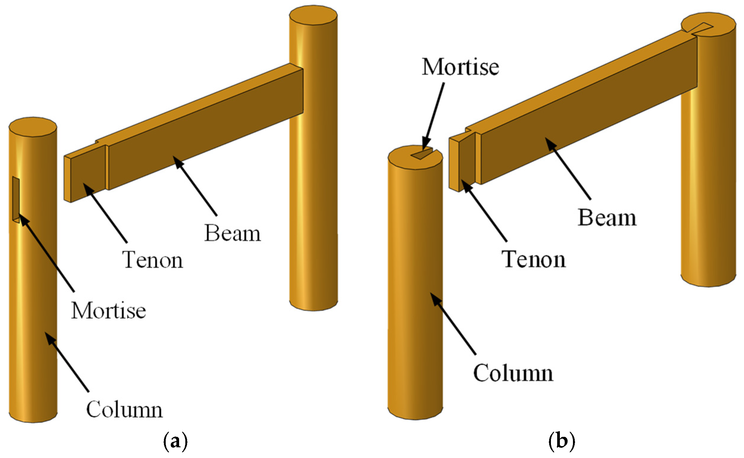
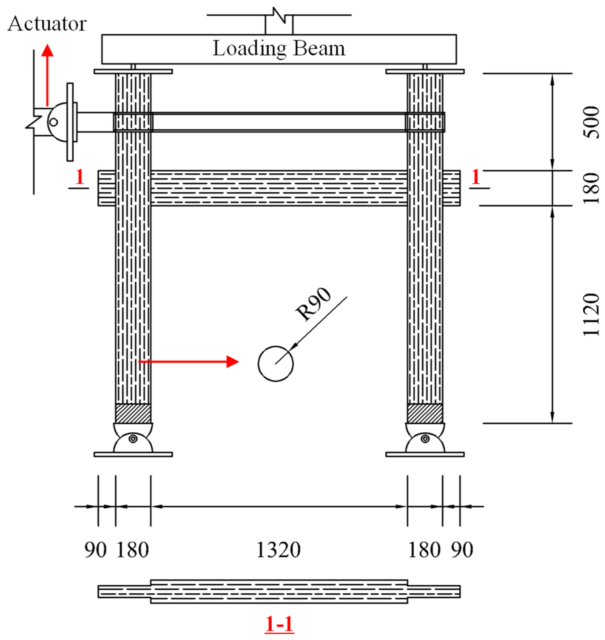
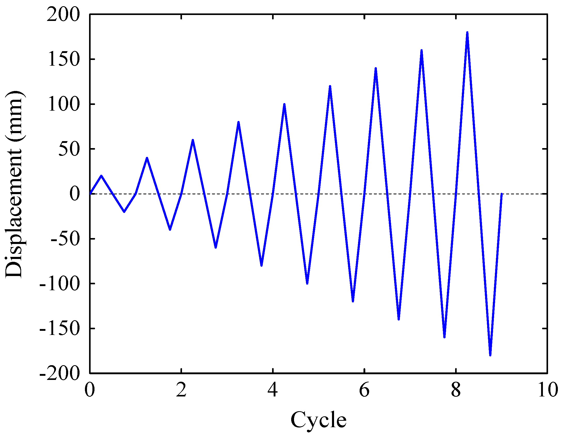
2.1. Test Model

The analytic model is derived from the quasi-static test of a traditional timber frame with straight mortise-tenon joints conducted by Lin [22]. The timber frame was designed based on Yingzaofashi [23], which is a technical code of practice for the construction of traditional timber buildings of the pre-Ming dynasty. The 1/3.52-scaled timber frame consists of two columns and a beam as shown in Figure 4. The columns are round with a diameter of 180 mm. The beam has a rectangular section of 120 mm × 180 mm, while the width of the tenon is only half of the beam, namely 60 mm. The bottom sides of both columns are hinged on the ground, which is consistent with the real situation that the columns are directly placed on the ground in most traditional timber structures. The vertical load of 10 kN is applied to the top of the columns through hydraulic jack to simulate the load transferred from the roof. The columns are driven by the MTS actuator through anchor bolt so that the columns can simultaneously move back and forth. More details of the test can be found in Lin [22].

The horizontal loading of the MTS actuator is controlled by displacement. A total of nine levels of displacement are taken in the test and each level consists of three cycles. The displacement amplitude is increased by 20 mm after each level of loading and the maximum displacement amplitude is 180 mm. Since the main purpose of the work is to study the influences of different types of damages on the seismic behavior of the timber frame, the loading cycle of each displacement amplitude is changed to one in the numerical simulation as shown in Figure 5 so as to reduce the calculation cost.

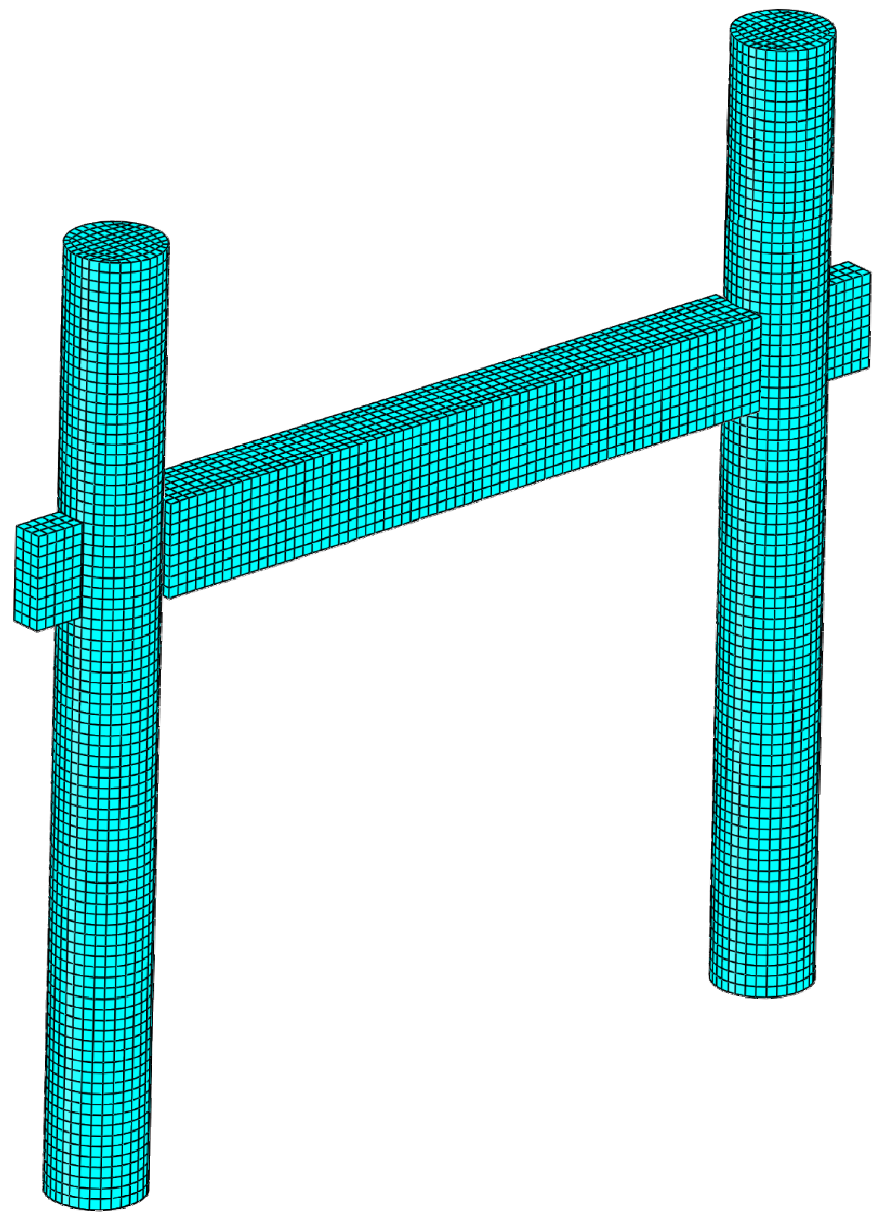
2.2. FE Model

To simulate the cyclic behavior of the timber frame with straight mortise-tenon joints, a 3D finite element model is built based on ABAQUS as shown in Figure 6. The columns and the beam are all modelled by 8-node reduced-integration solid element (C3D8R).

Timber is regarded as orthotropic material and the elastic behavior can be modelled through nine engineering constants, namely E₁, E₂, E₃, G₁₂, G₁₃, G₂₃, υ₁₂, υ₁₃, υ₂₃, which are Young’s moduli, Shear moduli, and Poisson’s ratios of three perpendicular directions. These elastic material parameters of the FE model are given in

Table 1. Elastic material parameters of the finite element (FE) mode.

E1/MPa	E2/MPa	E3/MPa	G12/MPa	G13/MPa	G23/MPa	υ12	υ13	υ23
4720	378	236	337	33.7	317	0.37	0.47	0.42

according to [13]. Here, subscript 1 means the direction of the grain, subscript 2 and 3 mean the radial and tangential direction in the plane perpendicular to the grain.

The post-yield behavior of timber is simulated through Hill’s potential function, which is a simple extension of the Mises function and can be expressed in terms of rectangular Cartesian stress components as follows:

$$f(\mathsf{\sigma })=\sqrt{F{({\sigma }_{22}-{\sigma }_{33})}^2+G{({\sigma }_{33}-{\sigma }_{11})}^2+H{({\sigma }_{11}-{\sigma }_{22})}^2+2L{\sigma }_{23}{}^2+2M{\sigma }_{31}{}^2+2N{\sigma }_{12}{}^2}$$

(1)

where F, G, H, L, M, N are constants obtained by tests of the material in different orientations, ${\sigma }_{ij}(i,j=1,2,3)$ are different stress components. For simplicity, the post-yield moduli are set as zero in this study. The plastic material parameters of the FE model are presented in

Table 2. Plastic material parameters of the FE mode.

Direction	${\mathit{\sigma }}_{\mathbf{cy}}$1 /MPa	${\mathit{\sigma }}_{\mathbf{ty}}$2 /MPa	${\mathit{\tau }}_{\mathbf{y}}$3 /MPa
1	21	30	4.2
2	2.1	2.1	4.2
3	2.1	2.1	4.2

¹ The yield compressive stress; ² The yield tensile stress; ³ The yield shear stress.

.

The interaction between the mortise and the tenon plays a significant role in the seismic performance of traditional timber structures since it can dissipate a vast amount of energy through friction between these two parts. In ABAQUS, the interaction between two surfaces is simulated by surface-to-surface contact which includes the normal and the tangential behaviors. The normal behavior is set as ‘HARD’ contact which can transfer the normal stress between the two surfaces and allow these two surfaces to separate after contact. The tangential behavior is realized by Coulomb friction to simulate the lateral sliding behavior at the interface of the mortise and tenon.

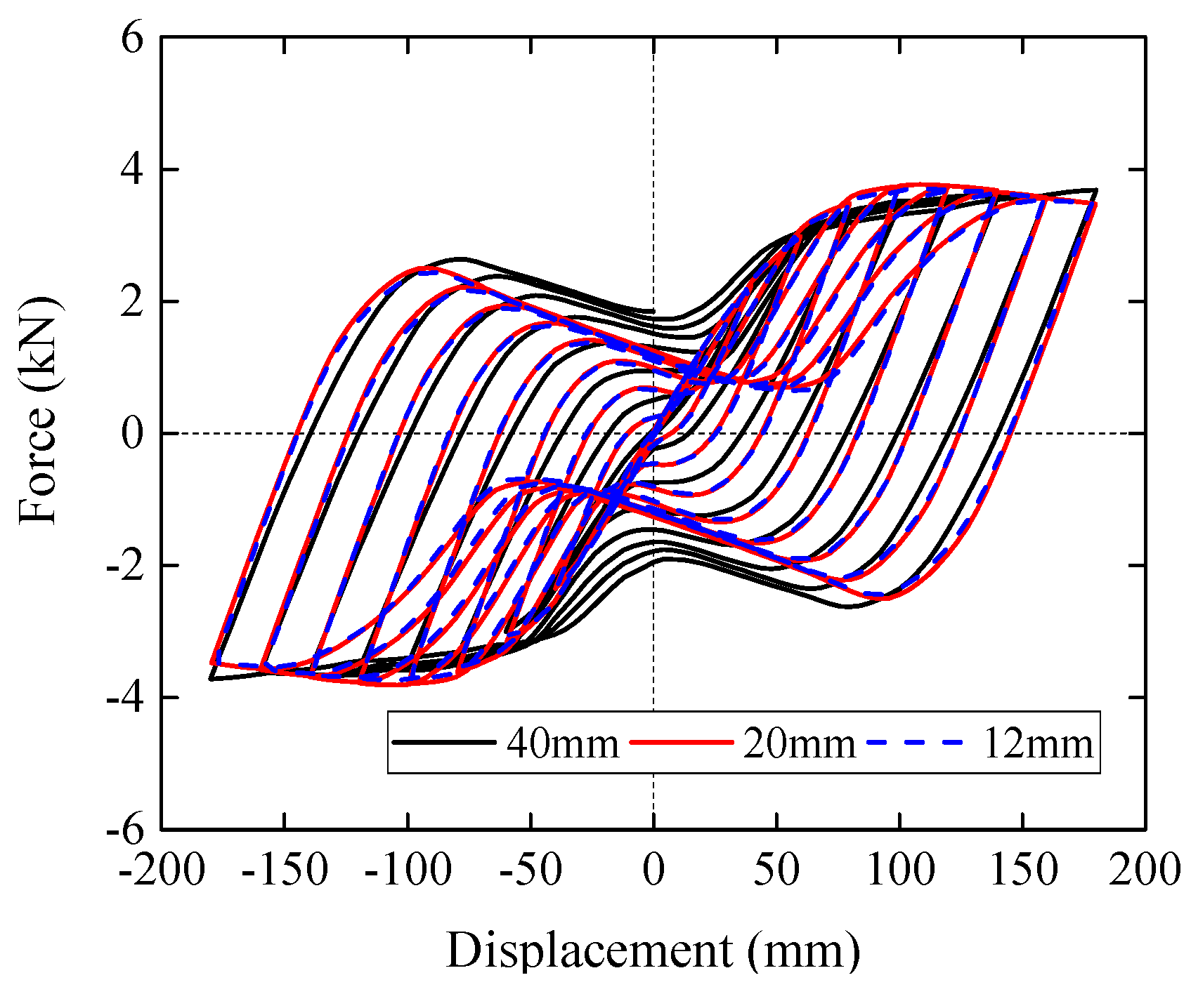
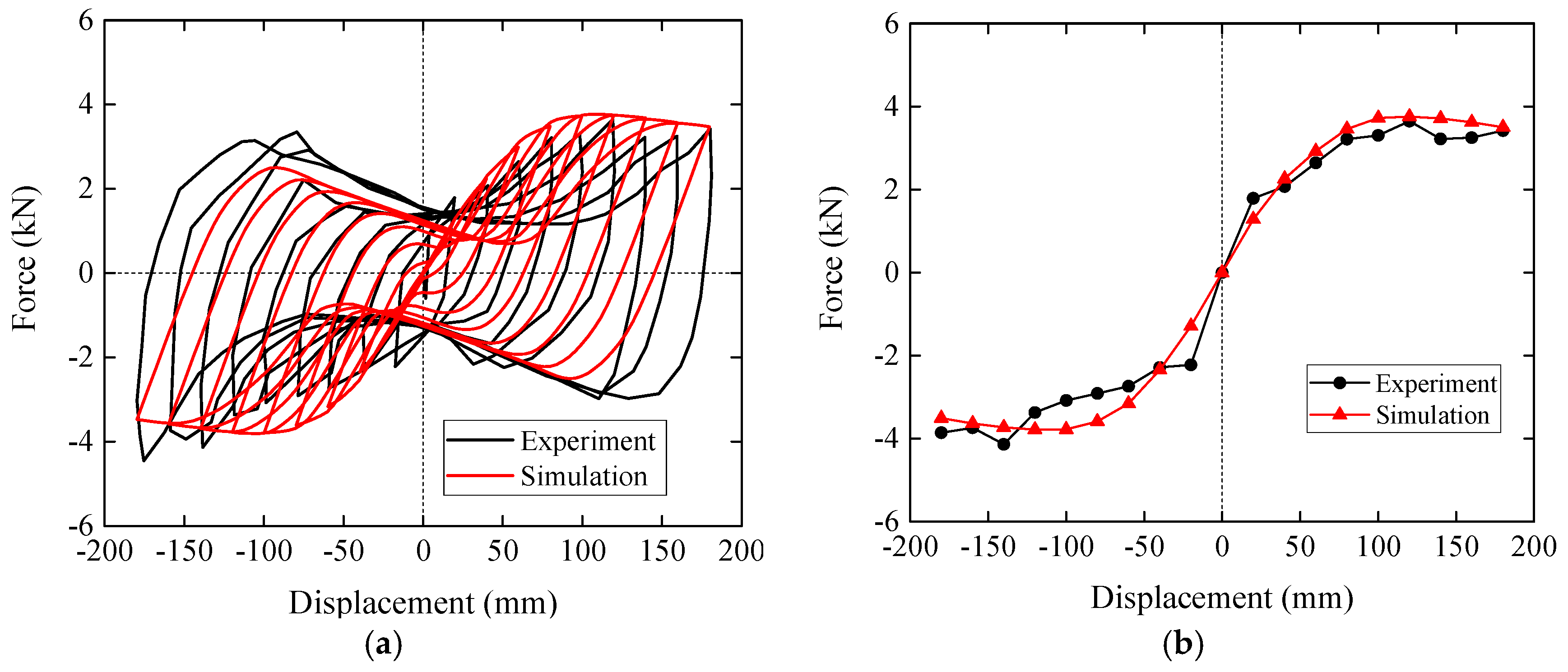
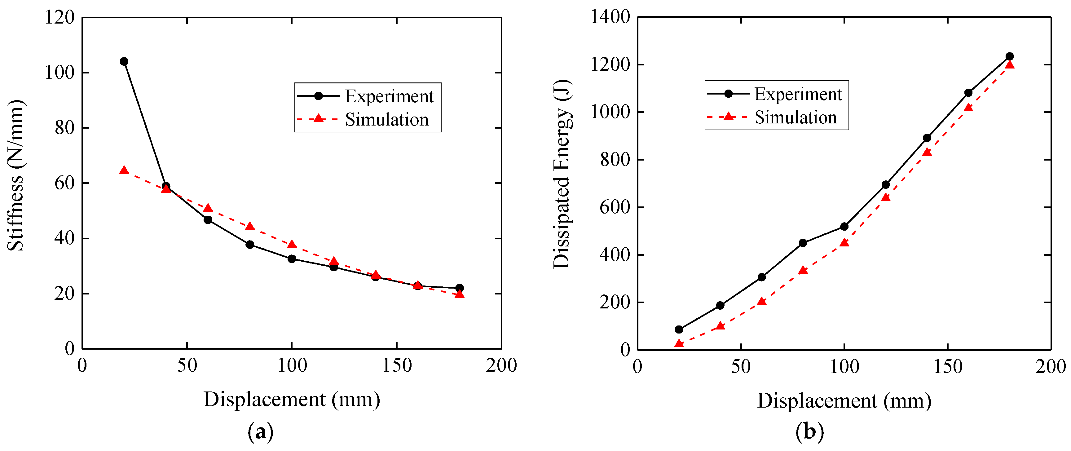
2.3. Verification

To verify the accuracy of the FE model, the mesh sensitivity analysis is first carried out so as to eliminate the adverse influence of element size on the calculation results. The element size of the FE model are set to be 40 mm, 30 mm, 20 mm and 12 mm, which results in the total element number of 3240, 6320, 21,666 and 90,720, respectively. The numerical simulation is run by a workstation installed with an Intel Xeon Gold 6154 CPU. The calculation time for each model is 35 min, 40 min, 72 min and 333 min.

The hysteresis curves of three models are plotted in Figure 7. It can be seen from the figure that the hysteresis curve of 20 mm model is nearly identical to that of 12 mm model, while the curve of 40 mm model is quite different from that of the model with the finest mesh. Therefore, the model with element size of 20 mm can be regarded as a preferable one and used in the following section since it provides almost the same results with the finest model and takes only 22% calculation time of the latter model.

The experimental hysteresis curves from Lin [22] and from the model with element size of 20 mm are plotted in Figure 8 for clearly comparison. It can be seen from Figure 8a that the hysteresis curve of this study is reversed Z-shaped and well reflect the pinch effect of the timber frame. However, the unloading stiffness is about 35% smaller than the experimental results, which is also seen in [24]. Figure 8b presents the skeleton curves of both experiment and simulation, and both of the curves show the nonlinear behavior when the displacement amplitude is larger than 20 mm. At the positive loading process, when the displacement reaches +120 mm, both skeleton curves begin to slightly decrease. While the descending displacements at the negative loading process of the experiment and the simulation are −140 mm and −120 mm, respectively.

During each cycle of loading, the stiffness is calculated according to Equation (2), in which $F_{i\max }$ is the force corresponding to the maximum positive displacement ${\Delta }_{i\max }$ in the ith cycle, and $F_{i\min }$ is the force corresponding to the maximum negative displacement ${\Delta }_{i\min }$ in ith cycle.

$$K({\Delta }_i)=\frac{\left|F_{i\max }\right|+\left|F_{i\min }\right|}{\left|{\Delta }_{i\max }\right|+\left|{\Delta }_{i\min }\right|}$$

(2)

For a given cycle i, the dissipated energy due to plastic deformation and friction equals to the area enveloped by the hysteresis curve.

Figure 9 shows the stiffness and dissipated energy of each cycle derived from both the experiment and the numerical results of this study. In Figure 9a, the two curves have the identical changing trend except the points of the first cycle. The error of 0.381 between the two points can be attributed to the tightness between the mortise and tenon during installation in the experiment, which exerts some pre-stress on the joints and leads to the increase of rotational stiffness of the experimental model. With the first point excluded, the numerical results well reflect the stiffness degradation of the timber frame. The dissipated energy of each cycle is plotted in Figure 9b, and it shows that the two curves have similar variation tendency, although the energy dissipation capacity of FE model is lower than the experiment. The hysteresis curves of the experiment when the displacement amplitude is less than 80 mm are full as can be seen in Figure 8a, while the enveloped curves of the simulation are reversed Z-shaped, which leads to the errors larger than 0.2. When the displacement amplitude reaches 100 mm, the errors are all within 0.15. Therefore, to a large extent, the FE model of this study can well simulate the hysteresis properties of the real timber frame with straight mortise-tenon joints.

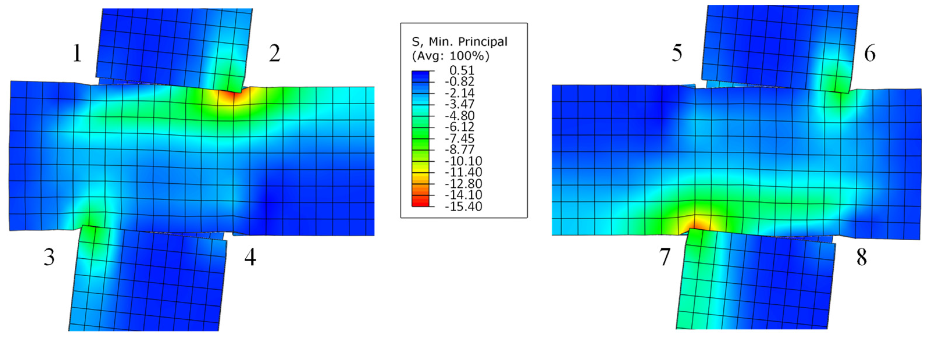
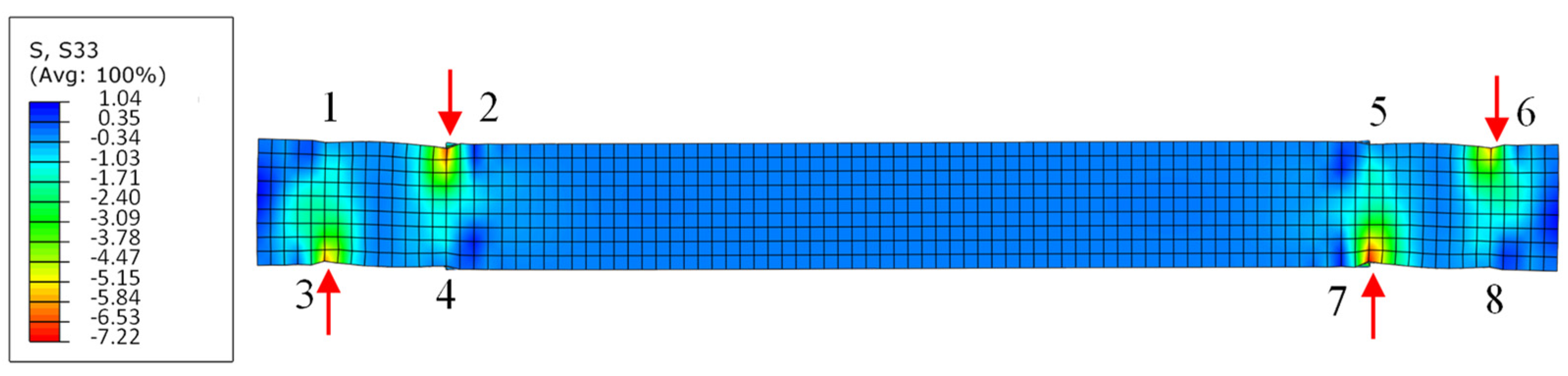
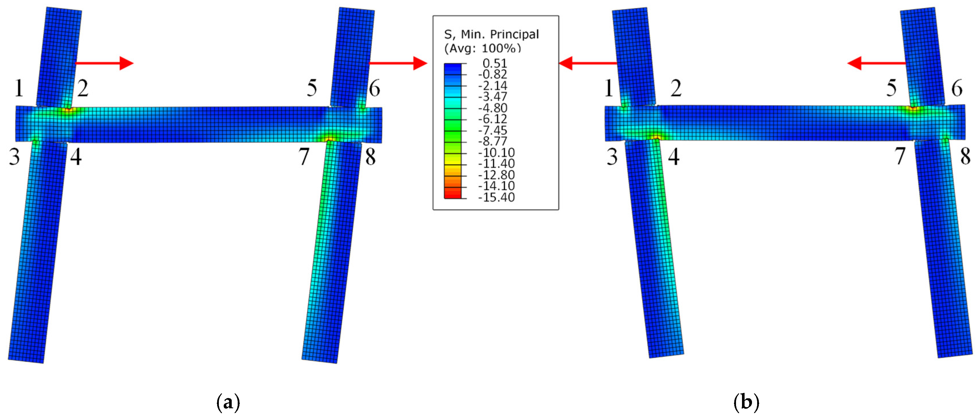
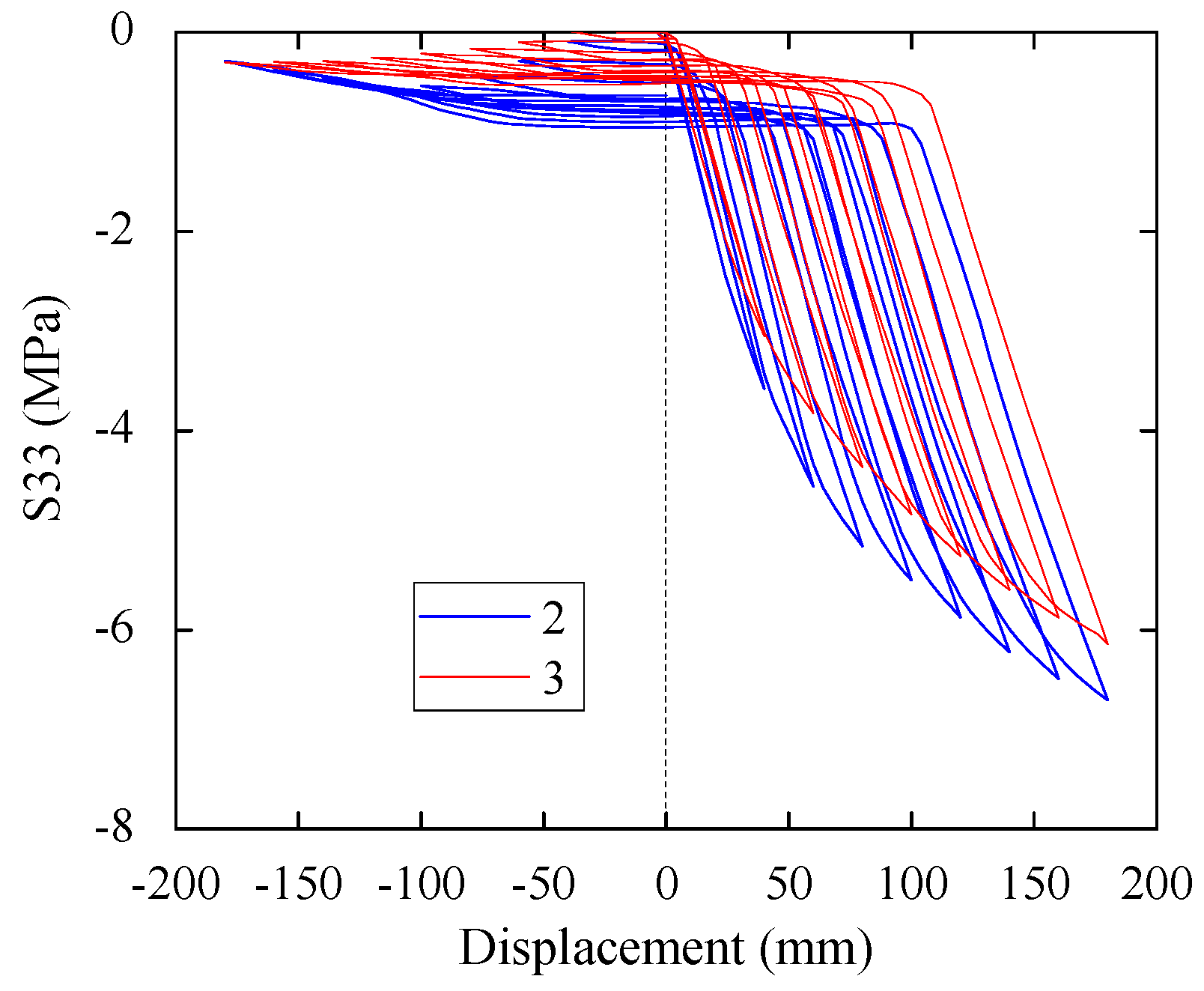
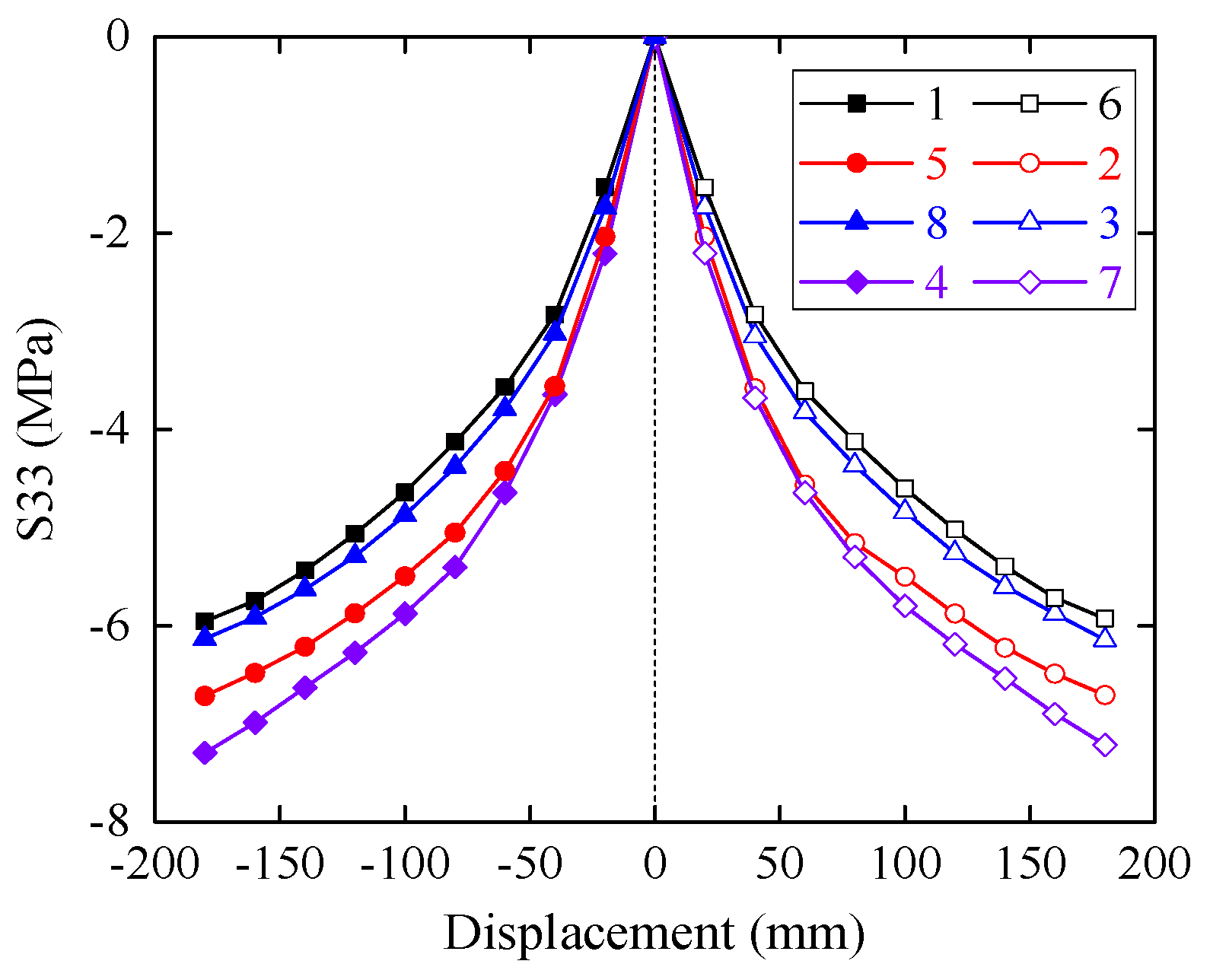
3. Stress Analysis

To clearly understand the deformative characteristics of the timber frame subjected to lateral cyclic loading, the deformed models and the minimum principal stress at the middle plane are plotted in Figure 10. Figure 10a,b show the compressive state of the frame under the displacement amplitude of +180 mm and −180 mm, respectively. It can be seen that since the frame is symmetrical, the two deformed models are also symmetrical.

The detailed deformed state of the mortise-tenon joints in Figure 10a is given in Figure 11. It can be seen that when the top of the columns are moving right at the displacement of +180 mm, the columns and the beam are in contact at the intersection points of 2, 3, 6 and 7. The largest value of compressive principal stress is 15.4 MPa at intersection point 2. When the displacement amplitude is −180 mm, the columns and the beam compress each other at the intersection points of 1, 4, 5 and 8, inversely, as shown in Figure 10b.

The vertical compressive stress in the beam, denoted as S33 in Figure 12, is vertical to the direction of the timber grain and is caused by the contact between the columns and the beam. Larger value of S33 in the beam means greater contact force derived from the column. If the contact forces exerted around the two intersection points of a mortise-tenon joint (for example intersection points 2 and 3) get larger, the bending moment caused by the two forces will also be greater, which then leads to more demand for the lateral loadings on the top of the columns.

Figure 13 shows the vertical compressive stresses S33 at the intersection points 2 and 3 with respect to the lateral loading displacement. It can be seen from the figure that when the timber frame moves left, the vertical compressive stresses are close to zero, which means the contact at these intersection points makes almost no contribution to the stiffness and strength of the timber frame. This is consistent with the phenomenon seen in Figure 10b. However, when the displacement amplitude increases from 0 mm to +180 mm, the envelope curve of S33 is similar to that of the reaction force of the timber frame, which confirms that larger values of S33 in the intersection points will demand greater lateral loadings on the top of the columns. Therefore, the envelope curves of S33 at all the eight intersection points are plotted in Figure 14. The symmetrical intersection points, for example 1 and 6, in the beam have the symmetrical envelope curves. At different displacement magnitudes, the vertical compressive stresses of intersection points 4 and 7 have larger values than those of other points.

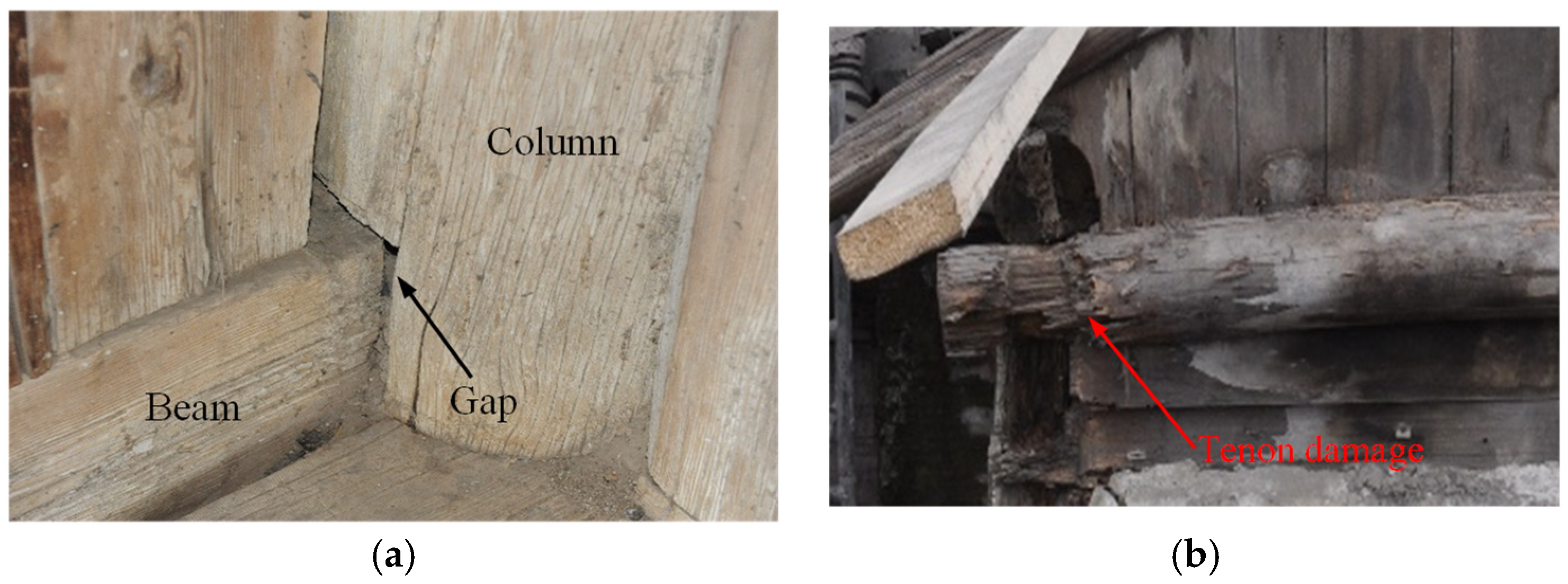
4. Damage of Mortise-Tenon Joint

To study the influences of mortise-tenon joint damages on the seismic performance of the timber frame. Three different types of damages are presented and idealized, so that the FE model can be modified accordingly.

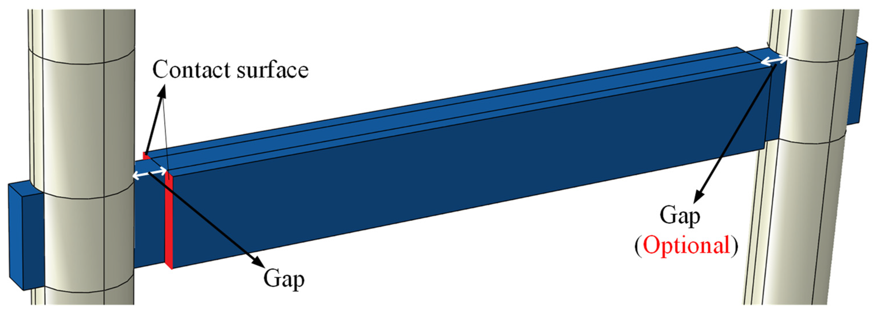
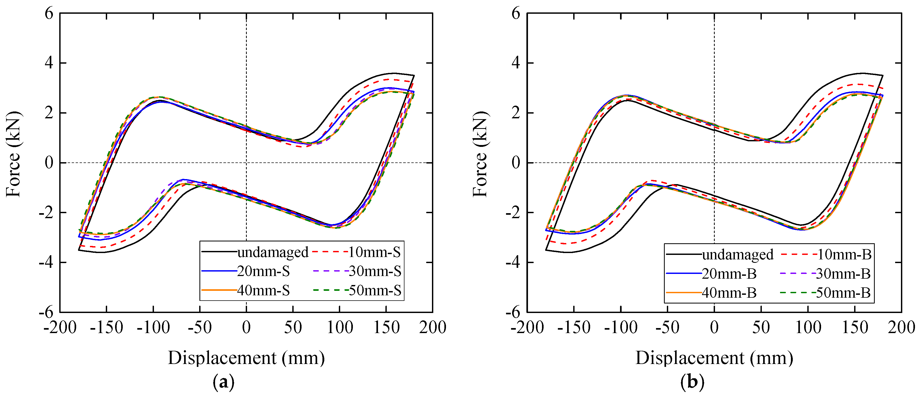
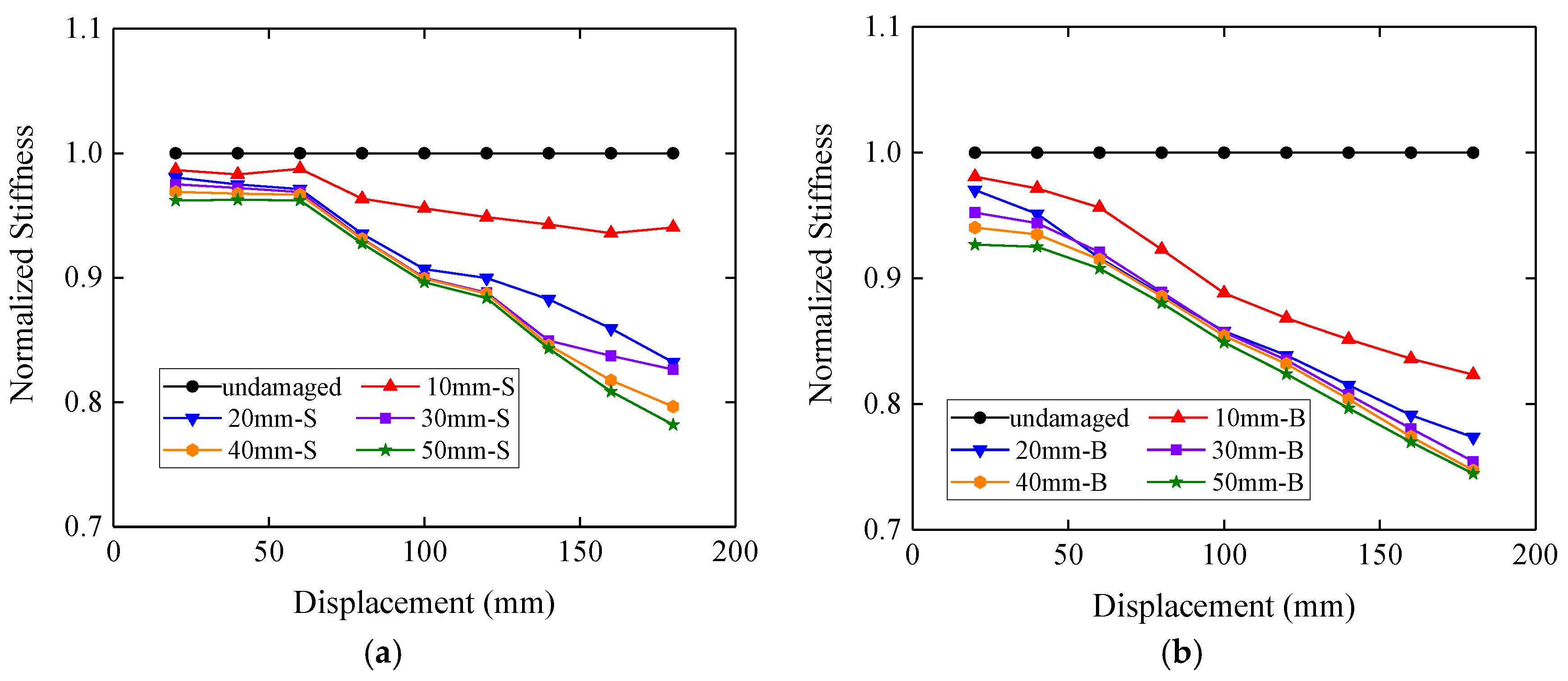
4.1. Gap between Mortise and Tenon

In this section, the beam and column are initially assembled with a gap in the left mortise-tenon joint of the frame or in both joints as illustrated in Figure 15. The preset gaps are 10 mm, 20 mm, 30 mm, 40 mm and 50 mm, which means 10 different models are analyzed herein. Different models are named by the length of the gap and a letter S (single joint damaged) or B (both joints damaged). For example, 40 mm-S model means the gap between the mortise and tenon of the left joint is 40 mm while the right joint is intact.

Figure 16 gives the hysteresis curves of the undamaged model and the damaged models when the displacement amplitude is 180 mm. It can be seen that the gap between the mortise and the tenon can decrease the maximum force and the stiffness of the timber frame. However, when the gap is larger than 20 mm, the maximum force and the stiffness will not change a lot with the increase of the gap. This is also clearly demonstrated in the normalized stiffness as shown in Figure 17. Here, the normalized stiffness is derived by dividing the stiffness of the damaged model by the stiffness of the undamaged model at the same displacement amplitude.

As is shown in Figure 17, when the displacement amplitude is small, the normalized stiffnesses of all damaged models are larger than 0.9. The normalized stiffness almost decreases linearly with the enlargement of the gap when the displacement amplitude is greater than 60 mm. From the comparison between these two figures, it can be concluded that when the length of the gap remains the same, the stiffness of the model with both joints damaged is slightly smaller than that of the model with only one joint damaged. When the gap reaches 20 mm, the normalized stiffness of these damaged models will become quite similar. This phenomenon can be attributed to the lack of contact between the external surface of the column and the vertical surface of the beam, which is marked by red in Figure 15. For the undamaged model, when the columns move back and forth, the external surfaces of the columns and the vertical surfaces of the beam will be in contact. The compressive stress of the vertical surface of the beam marked in Figure 15 is presented in Figure 18a when the displacement is +180 mm. If there is a gap between the column and the beam, the compressive stress between these surfaces will be smaller and even become zero, thus the maximum force and the stiffness of the frame will decrease. Figure 18b gives the compressive stress of the 10 mm-S model at the displacement of +180 mm, in which the maximum compressive stress is much smaller than that of the undamaged model. When the gap is larger than 10 mm, these surfaces will no longer squeeze with each other, therefore no compressive stress in the vertical surface of the beam is detected and the maximum force and the stiffness of these models are very close.

Similarly, the normalized dissipated energy is calculated by dividing the dissipated energy of the damaged model by that of the undamaged model at the same displacement, as is plotted in Figure 19. When the displacement amplitude is 20 mm, the total dissipated energy of each model is also very small, so that the lack of contact mentioned above has a great effect on the normalized dissipated energy and makes these values much bigger than the values of other displacement amplitudes. When the displacement amplitude is greater than 40 mm, the normalized dissipated energies of all damaged models are closely around a unit and the most reduction of the dissipated energy is about 9% at the displacement of 180 mm for single tenon damaged model and 160 mm for both tenon damaged model. Besides, the normalized dissipated energy slightly decreases with the increase of the displacement amplitude although some fluctuations are observed. This is because that in the loading process the reaction force of the undamaged model is larger than those of the damaged models, which makes the enveloped area of the undamaged model larger than the others; while in the unloading process, the reaction force of the undamaged model is still greater than the damaged models, which leads to the smaller enveloped area of the undamaged model, as can be seen in Figure 16. Therefore, the normalized dissipated energies of the damaged models are close to one when the displacement is larger than 40 mm.

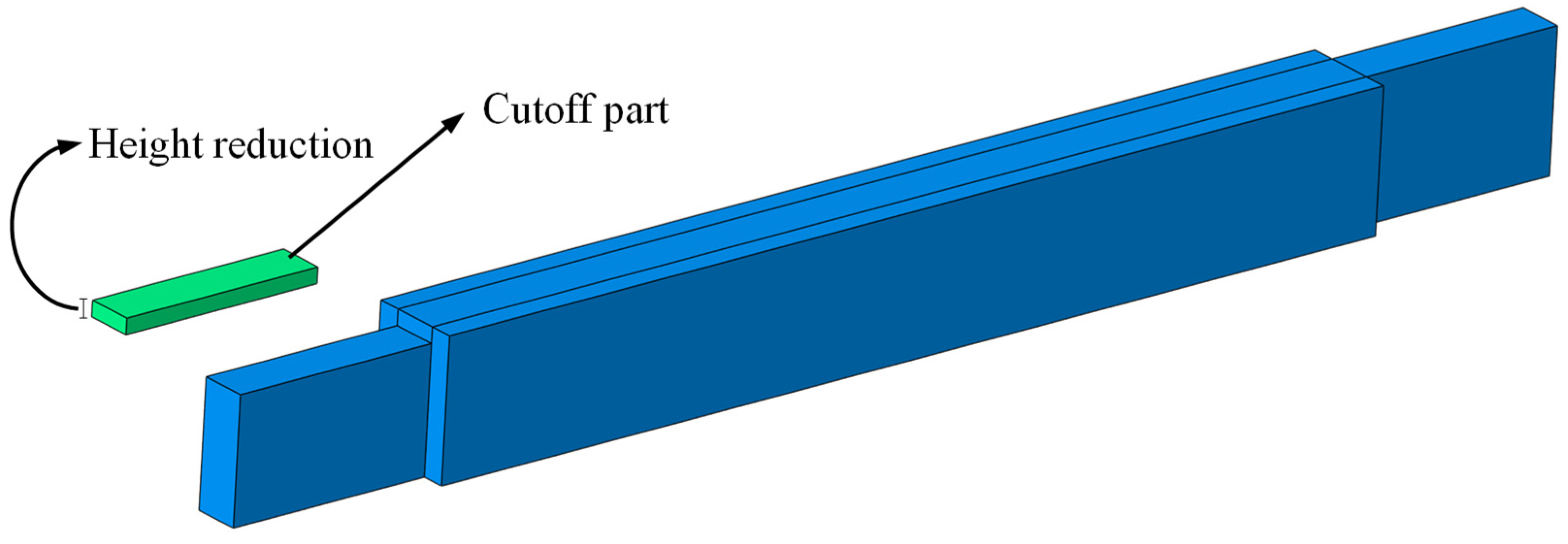
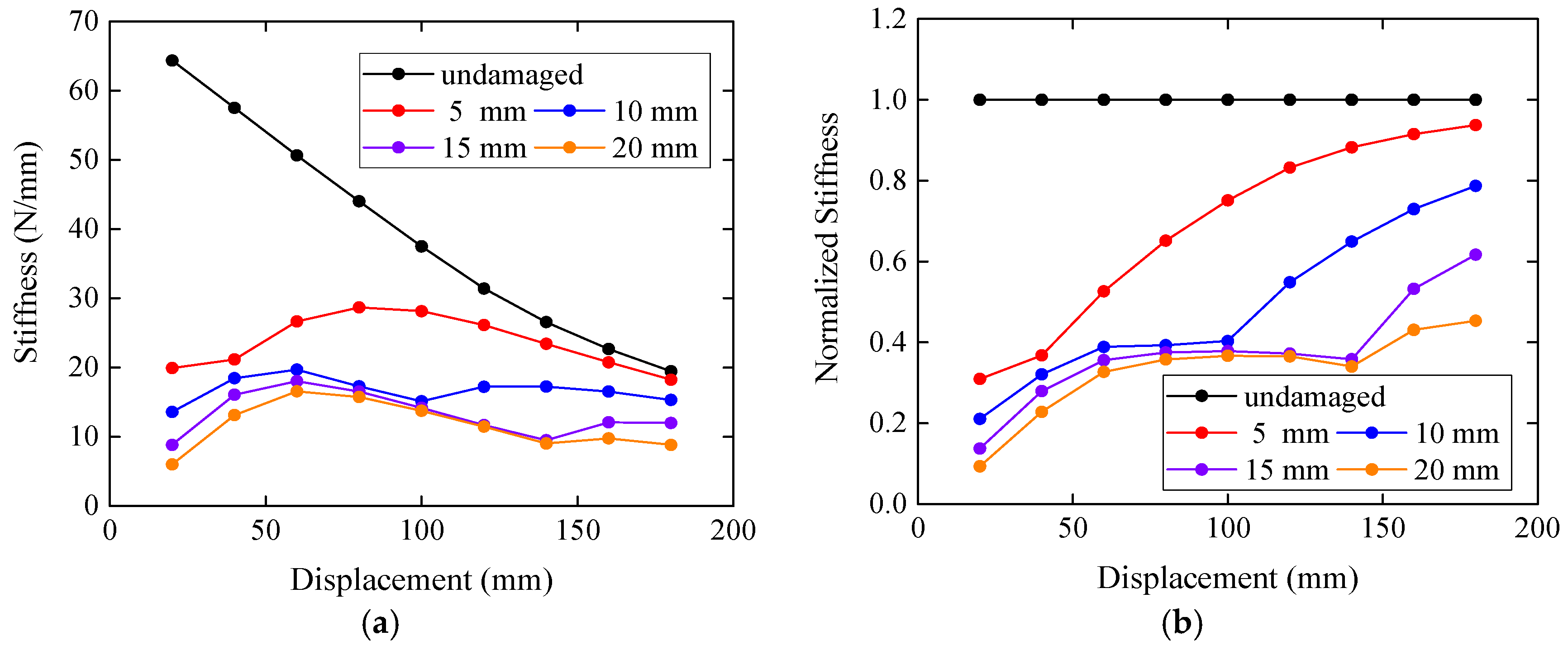
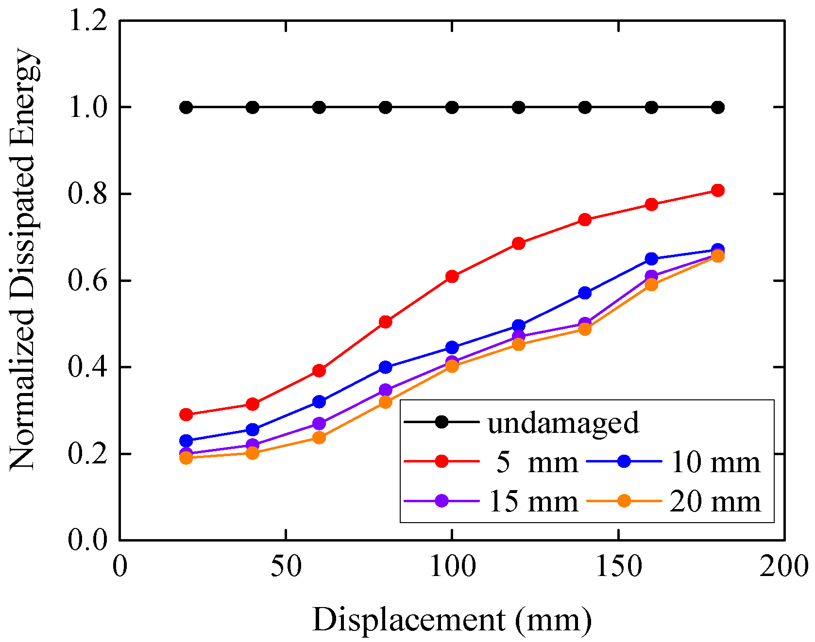
4.2. Damage in the Top of the Tenon

As can be seen in Figure 3b, the tenon part is often damaged and the cross-section of this part decreases a lot, especially in the upper place where the tenon and the mortise are in contact. In this section, this type of damage is simplified by reducing the height of the tenon of the left joint, with the length and width of the tenon remain unchanged, while the tenon of the right joint is not damaged, as shown in Figure 20. The original height of the tenon is 180 mm, and the reduction of the height is 5 mm, 10 mm, 15 mm and 20 mm.

The hysteresis curves of the damaged models as well as the undamaged one are plotted in Figure 21a, and the results of the last loading cycle are also given in Figure 21b for better comparison. It can be seen from both figures that the reaction forces at different displacement amplitudes of the damaged models are far smaller than those of the undamaged model, which indicates the smaller stiffness of the damaged models. Besides, the areas enveloped by the curves, which are known as dissipated energy, decrease with the increase of the reduction of the tenon.

The stiffnesses of each models are demonstrated in Figure 22a. For clear comparison between the stiffnesses of the undamaged model and the damaged models, the normalized stiffnesses are plotted in Figure 22b by dividing the stiffness of the damaged models by that of the undamaged model at the same displacement amplitude.

From these two figures, it can be concluded that the height reduction of the tenon can significantly decrease the stiffness of the damaged models, especially when the displacement amplitude is small. When the tenon is intact, it is initially in contact with the mortise, so that the interaction between the two parts works from the beginning. However, in the damaged models with a height reduction of the tenon, there is an empty space between the tenon and the mortise of the left joint, which indicates that the two parts are not in contact with each other at the very beginning. Therefore, the interaction between them takes effect when the columns moves laterally to different displacements for different height reductions of the tenon. Once the tenon and the mortise begin to squeeze each other, there will be a sudden increase in both the hysteresis curves and the stiffness curves, which can be seen in Figure 21 and Figure 22. It is clear in Figure 22b that the normalized stiffnesses of the damaged models with height reductions of 5 mm, 10 mm, 15 mm and 20 mm get larger prominently at the displacements of 40 mm, 100 mm, 140 mm and 140 mm, respectively. When these displacements are not reached by the corresponding models, the normalized stiffnesses of the damaged models are very close. For example, the normalized stiffnesses of the four damaged models at the displacement of 20 mm and 40 mm are around 0.2 and 0.3 respectively. Then, with the displacement increasing from 40 mm to 100 mm, the normalized stiffness of the 5mm-reduction model is much larger than those of other three models, while these three models have the similar normalized stiffness.

This phenomenon can be seen more directly from the vertical compressive stresses S33 plotted in Figure 23. Points 1–4 are the intersection points of the left mortise-tenon joint, while points 5–8 are related to the right joint, as can be seen in Figure 12. Since only the left joint is damaged, the envelope curves of S33 at points 1–4 of the damaged models are quite different from the curves of the undamaged model. When the displacement is small, the vertical compressive stresses S33 of the damaged models at these four points are nearly 0, which are far smaller than those of the undamaged model. When the tenon and the mortise of the left joint begin to squeeze each other, S33 at these four points will increase rapidly. For instance, from the envelope curve of S33 at point 1 of the 5 mm-reduction model, it can be inferred that the interaction between the tenon and the mortise starts to work when the displacement is up to 40 mm, which is identical with Figure 22.

The normalized dissipated energy is plotted in Figure 24 by dividing the dissipated energy of the damaged models at each displacement amplitude by the dissipated energy of the undamaged model at the same displacement amplitude. It can be seen from the figure that this type of damage can greatly reduce the energy dissipation capacity of the frame. When the displacement is small, the energy dissipation capacity of the damaged models can be only 1/5 of the undamaged one. The frame loses more energy dissipation capacity when the tenon suffers more reduction of the height. However, the normalized dissipated energy are similar for the damaged models with 10 mm, 15 mm, and 20 mm reduction, especially at the displacement of 180 mm. Unlike what is found in the normalized stiffness of the damaged models, the normalized dissipated energy increases almost linearly with the enlargement of the displacement without any sudden changes. As well, at the displacement of 180 mm, the reductions of the dissipated energy are 0.6 for the models with 10 mm, 15 mm, and 20 mm length reduction and 0.75 for the model with 5 length reduction.

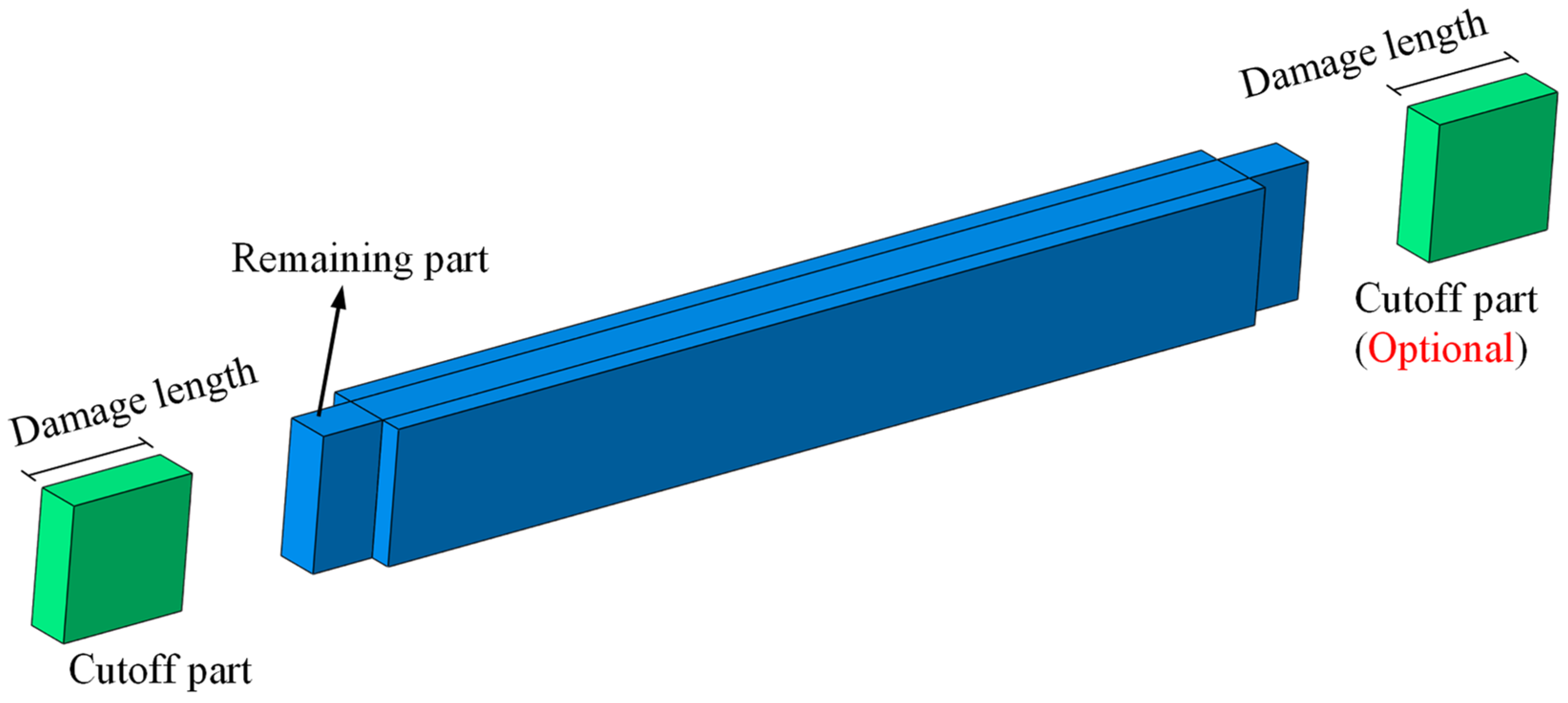
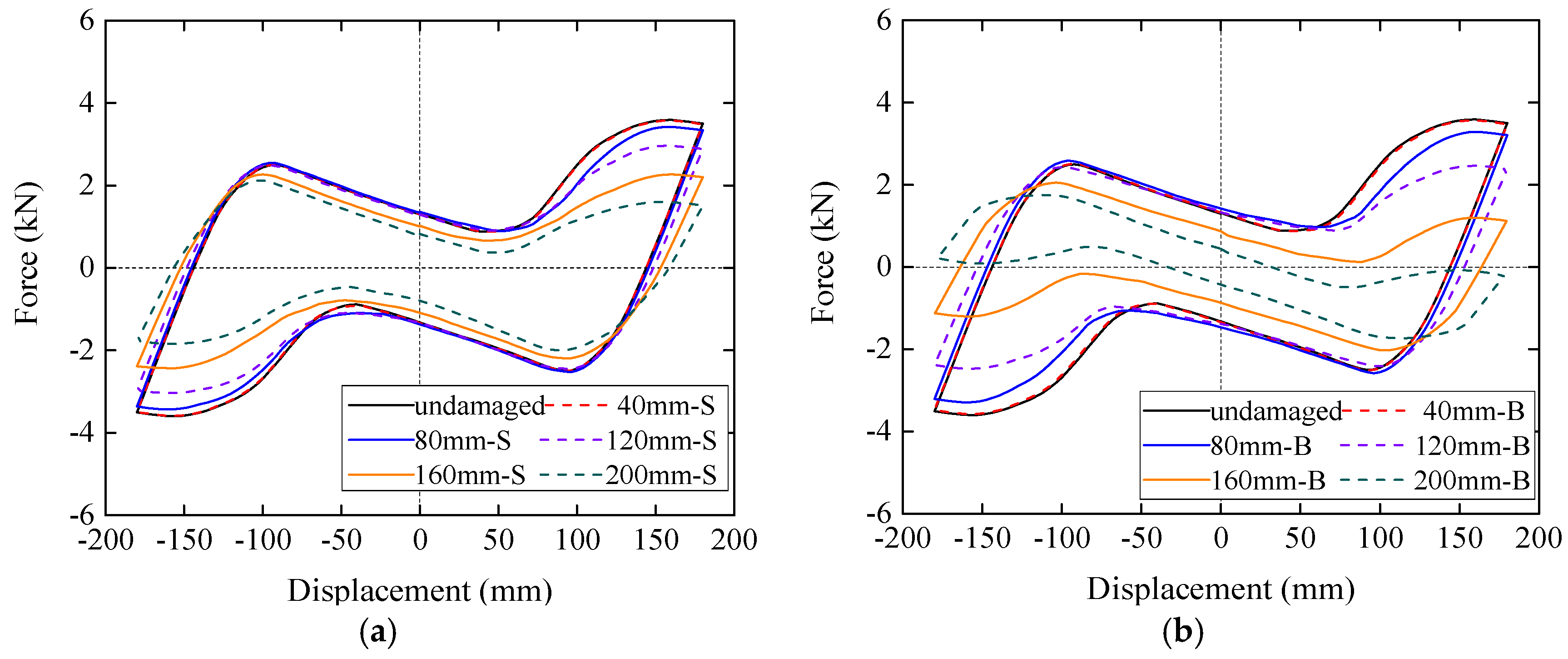
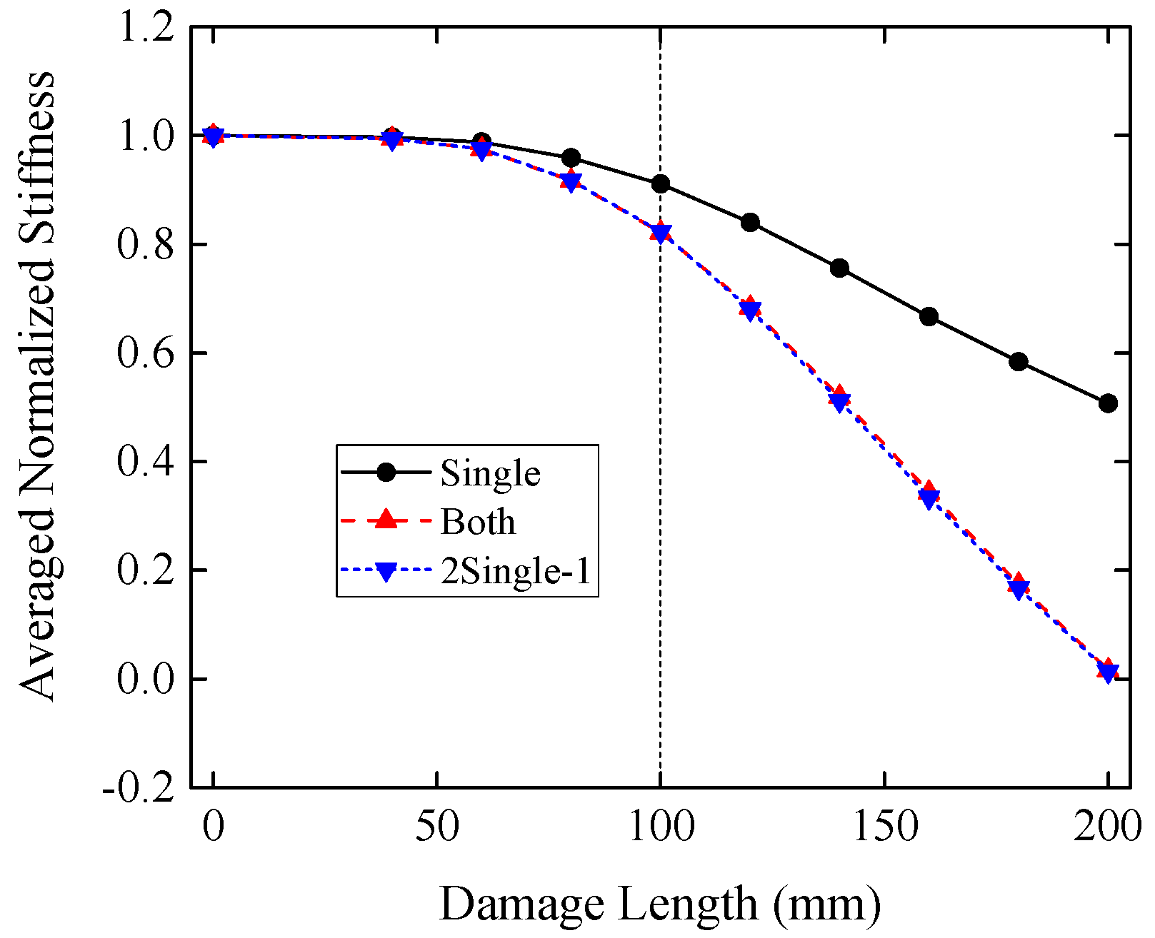
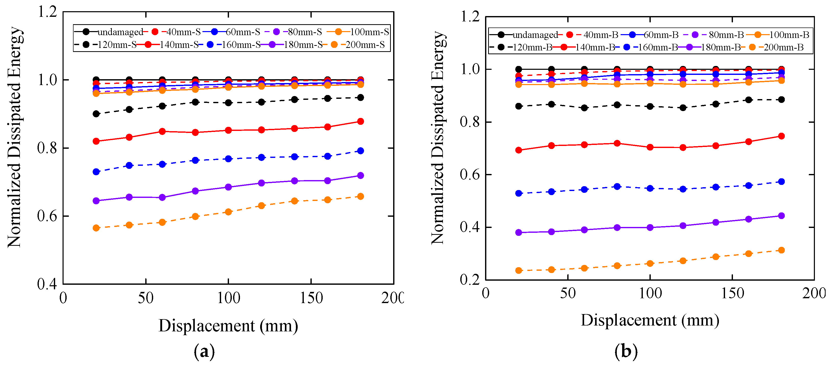
4.3. Damage in the End of the Tenon

In this section, the tenon is simplified to be cut off perpendicular to the longitudinal direction of the beam, as is seen in Figure 25. This cutoff damage is designated to happen in the left tenon or in both tenons. The damage length of the tenon is from 40 mm to 200 mm with intervals of 20 mm. Therefore, there are 18 damaged models generated in this section. Here, the damage length along with the letter S (for single tenon damaged) or B (for both tenons damaged) are used to denote the damaged models. For example, 40 mm-S model means that the damage length of the tenon is 40 mm and only the left tenon of the model is damaged. It should be noted that the length of the tenon exceeding the column is 100 mm, as seen in Figure 4. Therefore, when the damage length is bigger than 100 mm, the remaining part of the tenon is all inside the column.

The hysteresis curves of the last loading cycle of the damaged models as well as the undamaged model are given in Figure 26. It should be noted that not all curves derived from the damaged models are given in the figure since they share the similar varying trend. Figure 26a shows the results of the models that only have their left tenon damaged (labelled with S), while Figure 26b are related to the models with both tenons damaged (labelled with B). It can be seen from both figures that the 40 mm-S model and the 40 mm-B model have identical hysteresis curves with the undamaged model, which means this cutoff part contributes little to the strength and stiffness of the frame. This is consistent with the stress diagram in Figure 10 since the stress in that cutoff part is almost zero. Besides, the strength and the dissipated energy of the last cycle both reduce with the increase of the damage length of the tenon. From the comparison between these two figures, when the damage lengths are the same, the strength and the dissipated energy of the single tenon damaged model are greater than the model with two damaged tenons.

Figure 27 demonstrates the varying trend of the stiffness of the damaged and undamaged models. It can be seen from both figures that, at the same displacement amplitude, the stiffness of the damaged models gets smaller with the enlargement of the cutoff part. For the 200 mm-B model, negative stiffness is observed when the displacement amplitude reaches 140 mm, which is also seen in Figure 26b.

To better understand the influence of this cutoff damage on the stiffness of the model, the normalized stiffnesses of the damaged models are given in Figure 28. Although the normalized stiffness of different damaged models changes with respect to the displacement amplitude, the changing range of each curve is very limited. Therefore, the normalized stiffness of each model is regarded as a constant value, which is derived by averaging the normalized stiffnesses of the model at different displacement amplitudes, and is labelled as Averaged normalized stiffness (ANS) in

Table 3. Averaged normalized stiffness (ANS) of damaged models.

Damage Length (mm)		0	40	60	80	100	120	140	160	180	200
ANS	Single	1	0.997	0.988	0.959	0.911	0.840	0.756	0.667	0.584	0.507
	Both	1	0.994	0.975	0.917	0.822	0.684	0.519	0.353	0.174	0.016
2Single-1 1		1	0.994	0.976	0.917	0.823	0.680	0.512	0.334	0.167	0.014

¹ 2Single-1 means twice the values in the row of ‘Single’ and then subtract 1.

.

When the damage length is smaller than 100 mm, there is still some remaining part of the tenon outside the column. Therefore, the tenon of the damaged model contacts with the mortise at the abovementioned intersection points as the undamaged model. However, when the damage length exceeds 100 mm, the remaining part of the tenon is all surrounded by the column, which leads to the contact points between the tenon and the mortise moving to the inner of the column. Therefore, the varying trends of the averaged normalized stiffness with the damage length before and after 100 mm are quite different as plotted in Figure 29. When the damage length is 100 mm, the averaged normalized stiffnesses of the single tenon damaged model and the both tenons damaged model are 0.91 and 0.82, respectively. When the damage length is greater than 100 mm, the two curves are almost linear, and the slopes of the two curves are −0.00404 mm⁻¹ and −0.00806 mm⁻¹. The former value is nearly half of the latter one. This is because the slope can be regarded as the reduction of the stiffness of the damaged model. If a given damage length l causes a reduction $d_{\mathrm{S}}(l)$ on the averaged normalized stiffness of the single damaged model, then the averaged normalized stiffness ${\overline{NK}}_{\mathrm{S}}(l)$ of this model can be derived by

$${\overline{NK}}_{\mathrm{S}}(l)=1-d_{\mathrm{S}}(l)$$

(3)

When both of the tenons are damaged with the same damage length l, and the damages at the two tenons are not supposed to affect each other, thus the reduction on the averaged normalized stiffness will be $2d_{\mathrm{S}}(l)$, and the averaged normalized stiffness ${\overline{NK}}_{\mathrm{B}}(l)$ will be

$${\overline{NK}}_{\mathrm{B}}(l)=1-2d_{\mathrm{S}}(l)=1-2(1-{\overline{NK}}_{\mathrm{S}}(l))=2{\overline{NK}}_{\mathrm{S}}(l)-1$$

(4)

The right part of Equation (4) $2{\overline{NK}}_{\mathrm{S}}(l)-1$ is calculated and listed in the last row of Table 3 and is also plotted in Figure 29 labelled by 2Single-1. It can be seen that the $2{\overline{NK}}_{\mathrm{S}}(l)-1$ is almost identical with ${\overline{NK}}_{\mathrm{B}}(l)$.

Figure 30 presents the normalized dissipated energy of the models, and these curves share the similar characteristics with the normalized stiffness. The normalized dissipated energy has a slight rising trend, especially for the models with large damage length, although the slopes of these curves are negligible. Therefore, the averaged normalized dissipated energy is achieved through the same way as the averaged normalized stiffness and is given in

Table 4. Averaged normalized dissipated energy (ANDE) of damaged models.

Damage Length (mm)		0	40	60	80	100	120	140	160	180	200
ANDE	Single	1	0.995	0.985	0.979	0.975	0.930	0.850	0.764	0.682	0.612
	Both	1	0.991	0.975	0.960	0.946	0.866	0.714	0.549	0.406	0.268
2Single-1		1	0.990	0.970	0.958	0.950	0.861	0.699	0.528	0.364	0.225

and Figure 31.

Just as the averaged normalized stiffness, the changing trends of the averaged normalized dissipated energy with the damage length smaller and bigger than 100 mm are significantly different. The averaged normalized dissipated energy can be regarded as a bilinear curve with the two straight lines intersecting at the damage length of 100 mm, which is remarked by the dash line in Figure 31. The slopes of the left part of the curves are prominently smaller than those of the right part. When the damage length is 100 mm, the averaged normalized energy of both models are 0.975 and 0.946, respectively, which are greater than the averaged normalized stiffnesses with the same damage length. When the damage length is smaller than 100 mm, the reductions on the dissipated energy are all greater than 0.95, which means the damage length smaller than 100 mm has little effect on the frame. When the damage length reaches 180 mm, the reductions on dissipated energy of single and both damaged models are 0.612 and 0.268, respectively. Similarly, a curve labelled with 2Single-1 is also plotted in the figure, and it is very close to the curve representing the averaged normalized dissipated energy of the both tenons damaged models, although the difference between the two curves gets larger with the increase of the damage length.

5. Conclusions

In this study, a FE model of a timber frame with straight mortise-tenon joints is built and verified. The stress state of the model subjected to the lateral cyclic loading is then analyzed. Three damage types of the mortise-tenon joint are proposed and included in the FE model to study the influence of these damages on the cyclic performance of the timber frame. The conclusions are as follows.

(1).

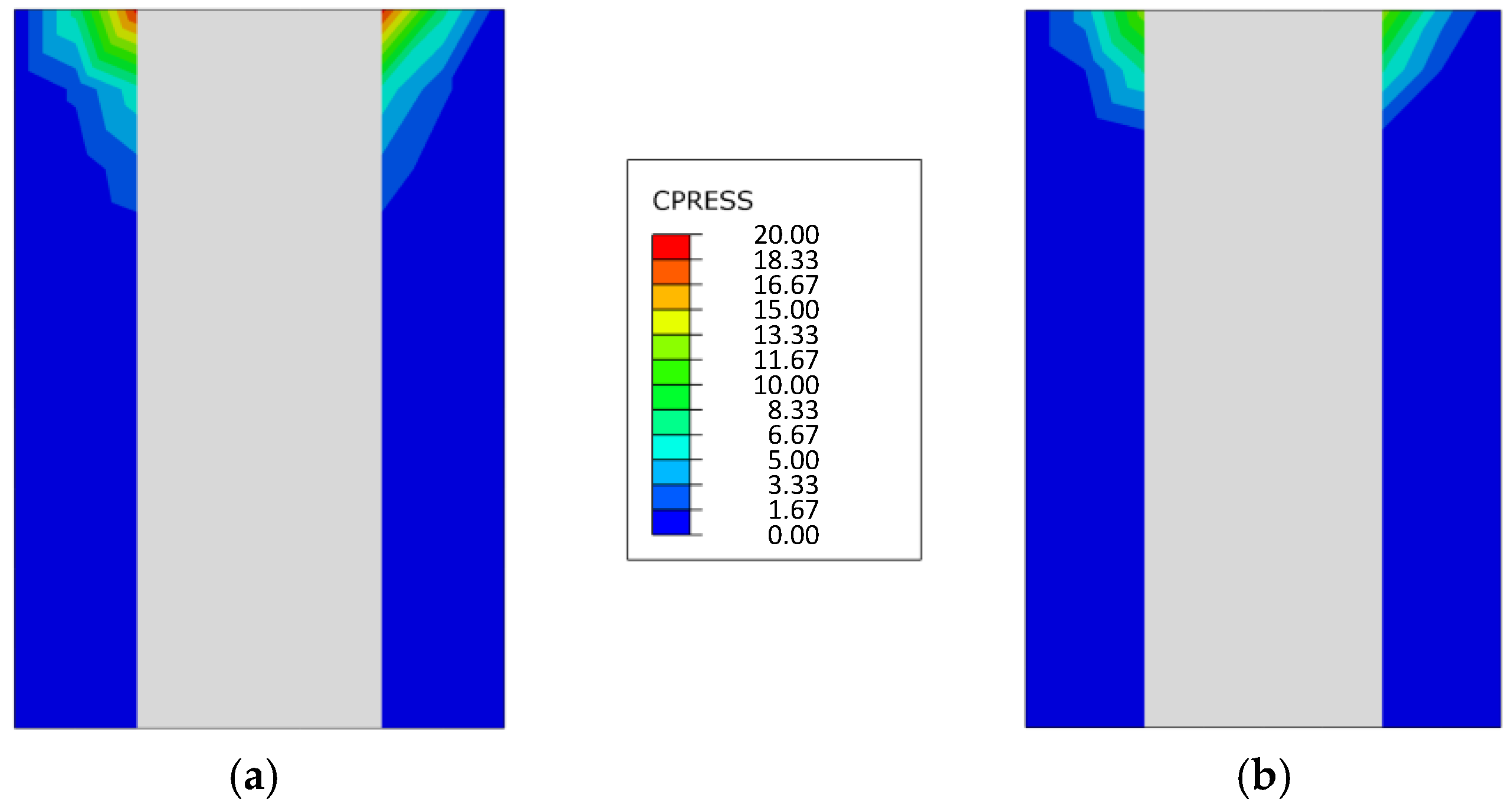
The vertical compressive stress at the contact surface of the mortise-tenon joint is a reasonable variable that can represent the reaction force of the whole model. Larger value of this stress corresponds to more demand for the lateral loadings exerted on the columns.

(2).

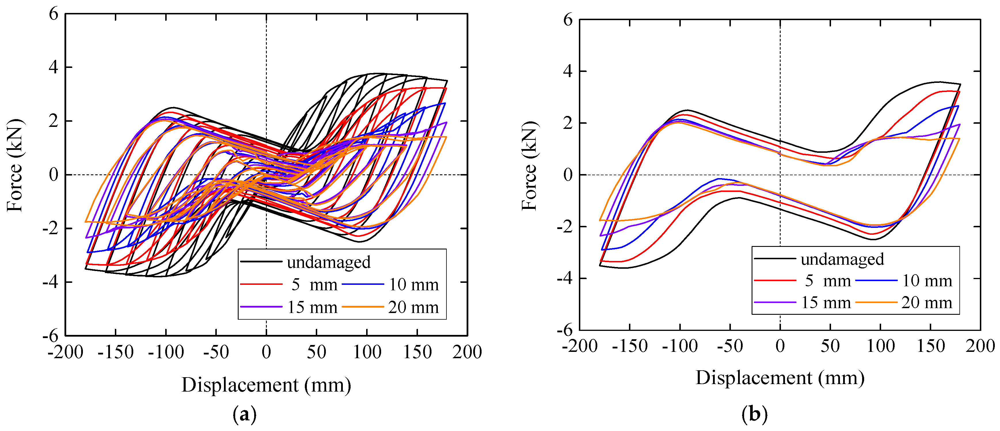
The gap between the mortise and the tenon can reduce the stiffness of the timber frame because of the lack of contact between the external surface of the column and the vertical surface of the beam, while the dissipated energy remains almost unchanged. When the gap reaches a certain value, 20 mm in this study, the stiffness will become stable.

(3).

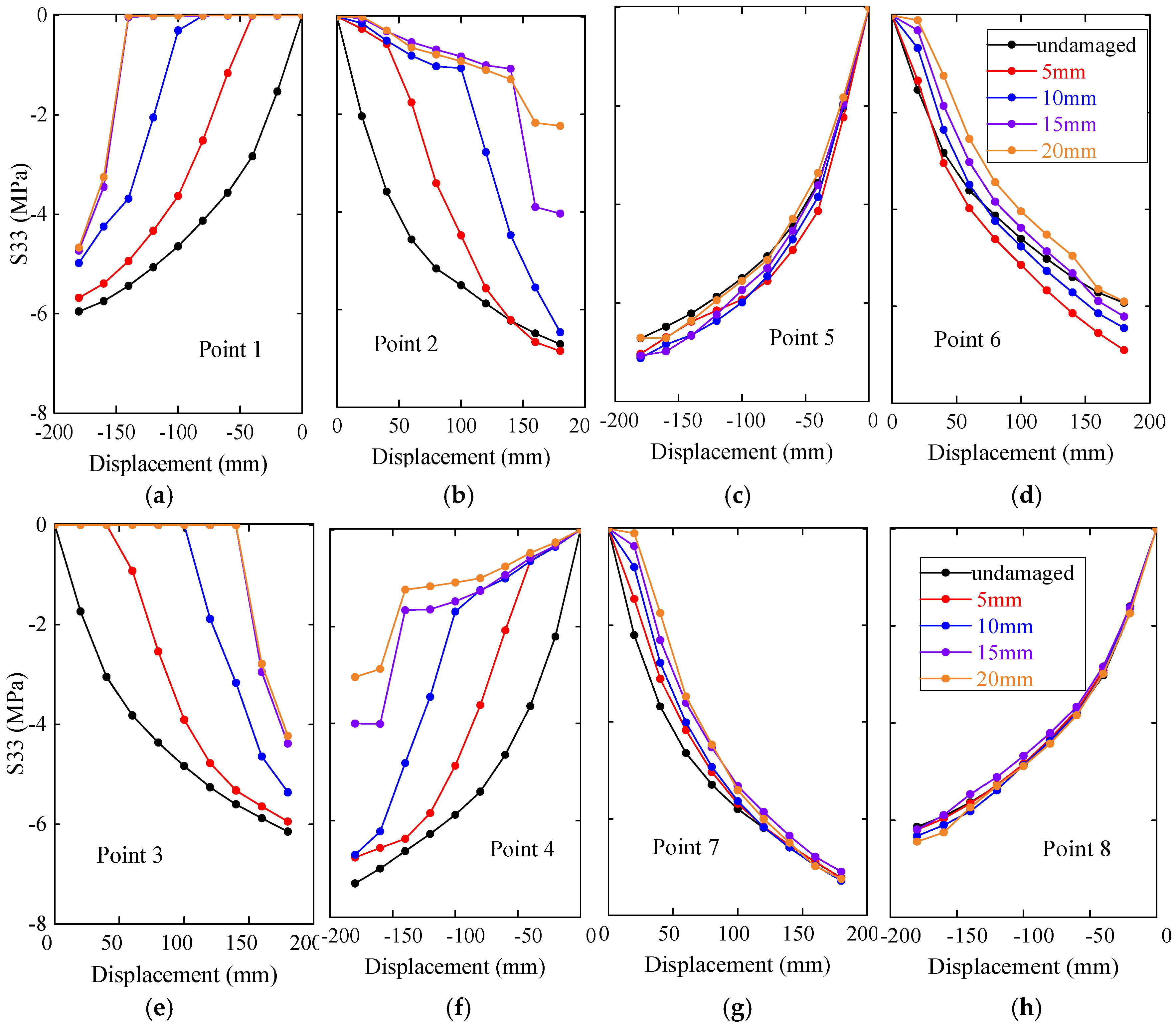
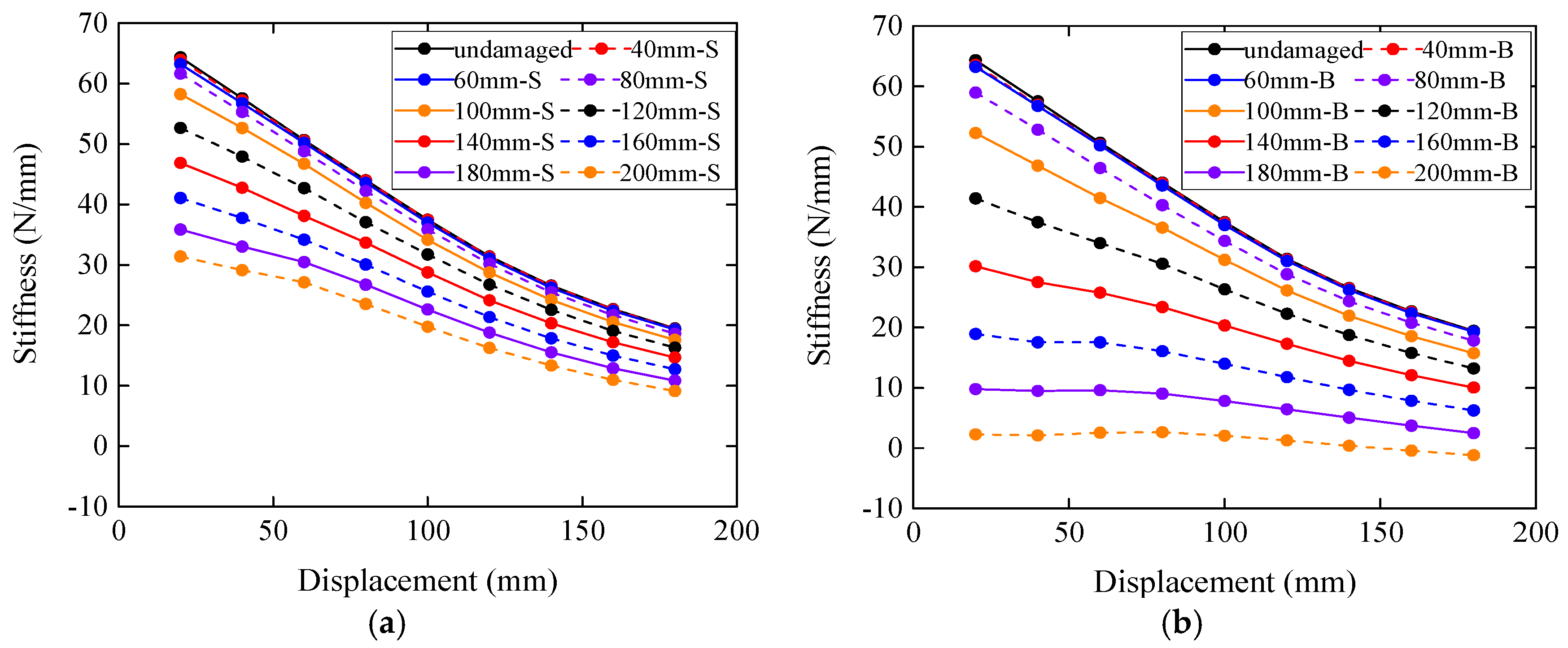
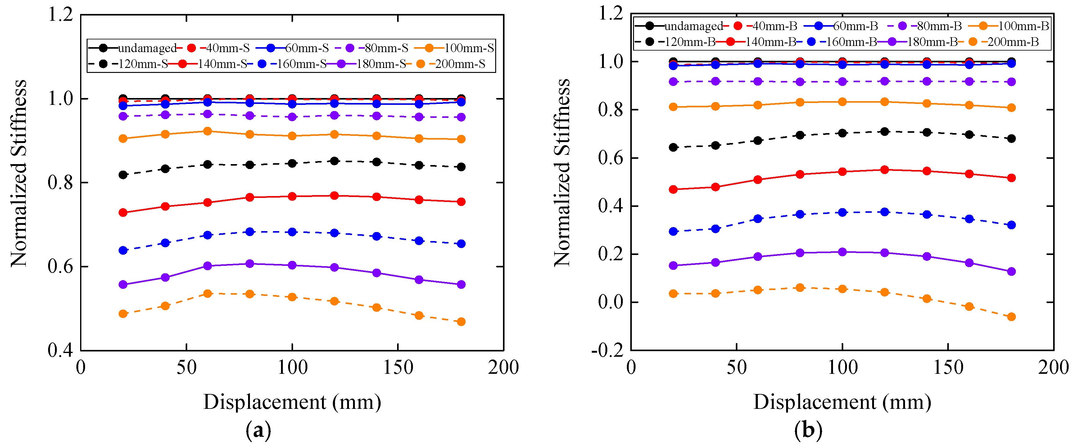
The damage in the top of the tenon can lead to the reduction in the maximum force and stiffness of the model followed by a sudden increase when some lateral displacement is reached. This certain lateral displacement can be derived from both the stiffness curves and the vertical compressive stresses at the contact surfaces.

(4).

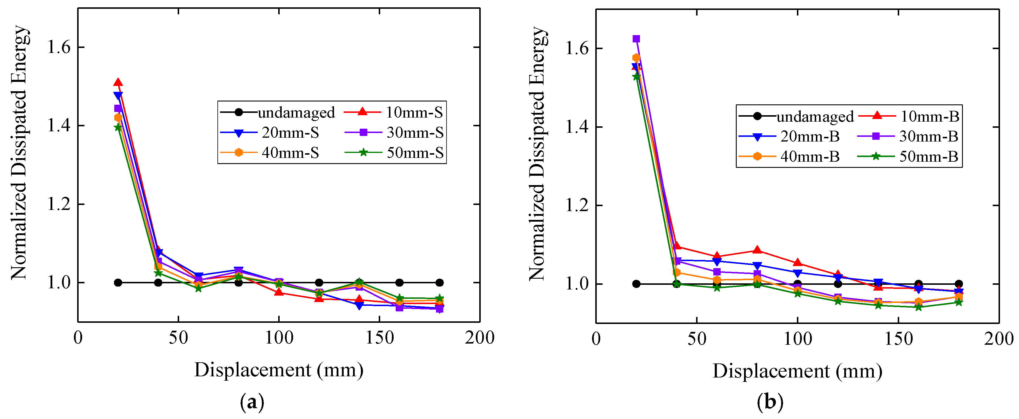
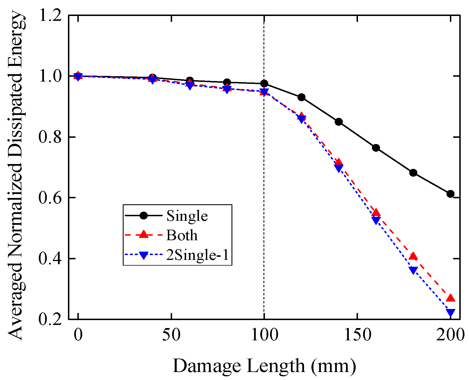
Damage in the end of the tenon has two types of influences on the stiffness and dissipated energy of the model according to the length of the cutoff part. When the length is small, the stiffness and dissipated energy decrease slowly with the increase of the length. When this length is larger than 100 mm in this study, the stiffness and dissipated energy will decrease dramatically.

References

- Fang, D.P.; Iwasaki, S.; Yu, M.H.; Shen, Q.P.; Miyamoto, Y.; Hikosaka, H. Ancient Chinese timber architecture. I: Experimental study. J. Struct. Eng. 2001, 127, 1348–1357. [Google Scholar] [CrossRef]
- Feio, A.O.; Lourenco, P.B.; Machado, J.S. Testing and modeling of a traditional timber mortise and tenon joint. Mater. Struct. 2014, 47, 213–225. [Google Scholar] [CrossRef]
- Xue, J.Y.; Xu, D.; Ren, G.Q.; Fu, C.W.; Yang, S.M. Earthquake simulation shaking table test of column-and-tie wooden structure dwellings. J. Build. Struct. 2019, 40, 123–132. (In Chinese) [Google Scholar]
- Xue, J.Y.; Wu, Z.J.; Zhang, F.L.; Zhao, H.T. Seismic damage evaluation model of Chinese ancient timber buildings. Adv. Struct. Eng. 2015, 18, 1671–1683. [Google Scholar] [CrossRef]
- Shi, X.W.; Chen, Y.F.; Chen, J.Y.; Yang, Q.S.; Li, T.Y. Experimental assessment on the hysteretic behavior of a full-scale traditional Chinese timber structure using a synchronous loading technique. Adv. Mater. Sci. Eng. 2018, 5729198. [Google Scholar] [CrossRef]
- Xie, Q.F.; Zhang, L.P.; Wang, L.; Zhou, W.J.; Zhou, T.G. Lateral performance of traditional Chinese timber frames: Experiments and analytical model. Eng. Struct. 2019, 186, 446–455. [Google Scholar] [CrossRef]
- Chun, Q.; Yue, Z.; Pan, J.W. Experimental study on seismic characteristics of typical mortise-tenon joints of Chinese southern traditional timber frame buildings. Sci. Chin. Technol. Sci. 2011, 54, 2404–2411. [Google Scholar] [CrossRef]
- Li, X.W.; Zhao, J.H.; Ma, G.W.; Chen, W. Experimental study on the seismic performance of a double-span traditional timber frame. Eng. Struct. 2015, 98, 141–150. [Google Scholar] [CrossRef]
- Li, X.W.; Zhao, J.H.; Ma, G.W.; Huang, S.H. Experimental study on the traditional timber mortise-tenon joints. Adv. Struct. Eng. 2015, 18, 2089–2102. [Google Scholar] [CrossRef]
- Seo, J.M.; Choi, I.K.; Lee, J.R. Static and cyclic behavior of wooden frames with tenon joints under lateral load. J. Struct. Eng. 1999, 125, 344–349. [Google Scholar] [CrossRef]
- Meng, X.J.; Li, T.Y.; Yang, Q.S. Experimental study on the seismic mechanism of a full-scale traditional Chinese timber structure. Eng. Struct. 2019, 180, 484–493. [Google Scholar] [CrossRef]
- Zhang, W.Z. The seismic and lateral resistance of column-and-tie wooden buildings based on mortise-tenon joint. Int. Wood Product J. 2019, 10, 86–91. [Google Scholar] [CrossRef]
- Jiang, S.F.; Wu, M.H.; Tang, W.J.; Liu, X.M. Multi-scale modeling method and seismic behavior analysis for ancient timber structures. J. Build. Struct. 2016, 37, 44–53. (In Chinese) [Google Scholar]
- Xiong, H.Y.; Tan, Z.R.; Zhang, R.H.; Zong, Z.J.; Luo, Z.P. Numerical calculation model performance analysis for aluminum alloy mortise-and-tenon structural joints used in electric vehicles. Compos. Part B Eng. 2019, 161, 77–86. [Google Scholar] [CrossRef]
- Sun, B.T.; Zhang, H.Y.; Yan, P.L. Earthquake damage and feature analysis of Chinese traditional timber frame structures subjected to the Lushan 7.0 earthquake. China Civ. Eng. J. 2014, 47, 1–11. [Google Scholar]
- Qu, Z.; Dutu, A.; Zhong, J.R.; Sun, J.J. Seismic damage to masonry-infilled timber houses in the 2013 M7.0 Lushan, China, earthquake. Earthq. Spectra 2015, 31, 1859–1874. [Google Scholar] [CrossRef]
- Xie, Q.F.; Wang, L.; Zheng, P.J.; Zhang, L.P.; Hu, W.B. Rotational behavior of degraded traditional mortise-tenon joints: Experimental tests and hysteretic model. Int. J. Archit. Herit. 2018, 12, 125–136. [Google Scholar] [CrossRef]
- King, W.S.; Yen, J.Y.R.; Yen, Y.N.A. Joint characteristics of traditional Chinese wooden frames. Eng. Struct. 1996, 18, 635–644. [Google Scholar] [CrossRef]
- Xue, J.Y.; Li, Y.Z.; Xia, H.L.; Sui, Y. Experimental study on seismic performance of dovetail joints with different loose degrees in ancient buildings. J. Build. Struct. 2016, 37, 73–79. (In Chinese) [Google Scholar]
- Xue, J.Y.; Guo, R.; Qi, L.J.; Xu, D. Experimental study on the seismic performance of traditional timber mortise-tenon joints with different looseness under low-cyclic reversed loading. Adv. Struct. Eng. 2019, 22, 1312–1328. [Google Scholar] [CrossRef]
- Li, S.C.; Jiang, Z.J.; Luo, H.Z.; Zhang, L. Seismic behavior of straight-tenon wood frames with column foot damage. Adv. Civ. Eng. 2019, 1–10. [Google Scholar] [CrossRef]
- Lin, M.Y. Experimental Research on Mechanical Property of Mortise-Tenon Joint of Chinese Ancient Timber Buildings. Master’s Thesis, Fuzhou University, Fuzhou, China, June 2014. (In Chinese). [Google Scholar]
- Li, J. Yingzaofashi; People’s Publishing House: Beijing, China, 2011. (In Chinese) [Google Scholar]
- Xie, Q.F.; Zhang, L.P.; Li, S.; Zhou, W.J.; Wang, L. Cyclic behavior of Chinese ancient wooden frame with mortise-tenon joints: Friction constitutive model and finite element modelling. J. Wood Sci. 2018, 64, 40–51. [Google Scholar] [CrossRef]