Article

Adaptive Backstepping Fractional Fuzzy Sliding Mode Control of Active Power Filter

Jiangsu Key Laboratory of Power Transmission and Distribution Equipment Technology, College of IoT Engineering, Hohai University, Changzhou 213022, China
*
Author to whom correspondence should be addressed.
Appl. Sci. 2019, 9(16), 3383; https://doi.org/10.3390/app9163383
Submission received: 23 July 2019 / Revised: 9 August 2019 / Accepted: 13 August 2019 / Published: 16 August 2019
(This article belongs to the Special Issue Control and Soft Computing)

Abstract

:
An adaptive fractional-order fuzzy control method for a three-phase active power filter (APF) using a backstepping and sliding mode controller is developed for the purpose of compensating harmonic current and stabilizing the DC voltage quickly. The dynamic model of APF is changed to an analogical cascade system for the convenience of the backstepping strategy. Then a fractional-order sliding mode surface is designed and a fuzzy controller is proposed to approximate the unknown term in the controller, where parameters can be adjusted online. The simulation experiments are conducted and investigated using MATLAB/SIMULINK software package to verify the advantage of the proposed controller. Furthermore, the comparison study between the fractional-order controller and integer-order one is also conducted in order to demonstrate the better performance of the proposed controller in total harmonic distortion (THD), a significant index to evaluate the current quality in the smart grid.

1. Introduction

With the development of power grids, more and more problems occur, accompanied by convenience and benefits. While power grids and distribution networks are desired to simultaneously interact with a large quantity of loads, the increasing number of nonlinear loads connected to the grids has caused a negative effect on the quality of electric power supply such as low power factor, electrical harmonics, and so on. Instead of a passive filter, the active power filter (APF) is a new power electronic device used for its higher flexibility and better capability of suppressing harmonic currents.
Due to the wide range of applications of APF in power systems over the past decades, many scholars have applied a variety of intelligent control methods to APF. Ouadi et al. [1] developed a new oriented control model for shunt active power filter (SAPF)-load system, and designed an adaptive controller based on the new model. Kale et al. [2] proposed a new robust adaptive controller based on shunt active power filters, to reduce high overshoot and large settling time in the DC link voltage. Fei et al. [3], Chu et al. [4], Fang et al. [5], and Fei et al. [6] investigated intelligent control methods such as an adaptive neural network controller and fuzzy neural controller for an active power filter to track command current to eliminate the harmonic current and improve the power quality of the power system. Gregory et al. [7] presented a SAPF configuration and showed advantages of harmonic distortion and power converter losses. Dey et al. [8] presented a D-Q current control method using a phase lock loop to improve the power quality.
Recently, fractional calculus as well as its application begins to attract more and more attention. In the last three decades, many engineers have applied fractional calculus and fractional differential equation theory with various applications [9,10,11,12,13,14]. Backstepping control techniques are powerful tools for their systematic and recursive design methodology for nonlinear feedback control [15,16,17,18]. Adaptive fractional fuzzy sliding mode controls and adaptive fuzzy-neural fractional finite-time sliding controllers are developed for active power filters [19,20,21]. In the nonlinear systems, unknown nonlinearities can be approximated by intelligent methods such as fuzzy systems [22,23,24,25,26,27,28,29] and neural networks [30,31,32,33,34,35]. Intelligent control methods have been investigated for dynamic systems. Motivated by the above literature, in this paper, a fractional adaptive backstepping sliding mode control method combined with fuzzy controller for a three-phase APF is proposed. The main motivations are emphasized as follows:
(1)
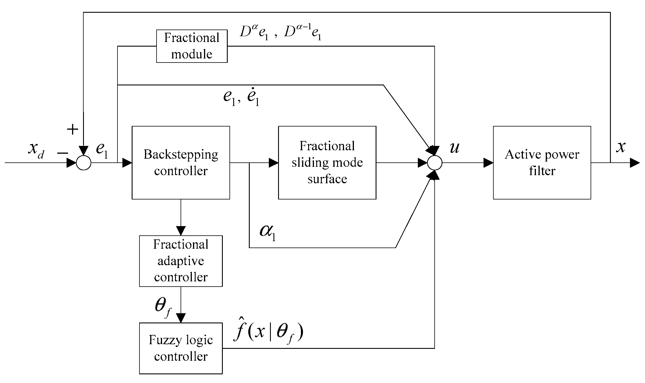
A backstepping control strategy is applied to the design of a fractional sliding mode adaptive fuzzy controller. We avoid establishing a precise mathematical model of active power filter by transforming the general circuit equation into an analogical cascade system where the backstepping approach can be implemented.
(2)
Based on the backstepping control design, this paper extends the conventional integer-order sliding surface to fractional ones for three-phase active power filter. That means the system can achieve an extra degree of freedom and there would be more parameters to be adjusted to improve total harmonic distortion (THD).
(3)
A fractional sliding mode controller ensures that the control system reaches the sliding surface while the adaptive control strategy and fuzzy controller are also combined together to approximate the unknown dynamic model term and identify adaptive parameters online.

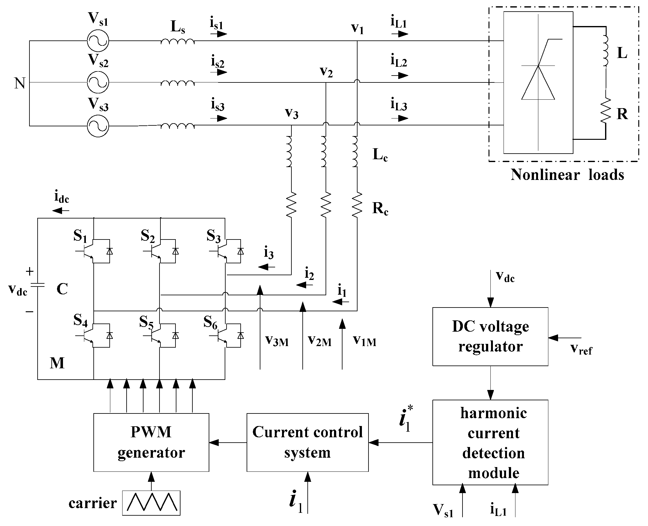
2. System Description

The three-phase shunt active power filter has the structure of Figure 1, composed of a harmonic current detection module, control system, and main circuit.
In Figure 1, v s 1 , v s 2 , v s 3 , are the grid voltages, i s 1 , i s 2 , i s 3 are the power currents, i L 1 , i L 2 , i L 3 are the load currents, v 1 , v 2 , v 3 are the voltages of public join points, i 1 , i 2 , i 3 are the compensation current of APF, C is the capacitor of DC side, v d c is the voltage of C, i d c is the current of C, L c is the inductance of AC side, and R c is the equivalent resistance.
The model of the APF will be given in the following steps. Applying Kirchhoff rules to the system, we can get the following equations:
{ v 1 = L c d i 1 d t + R c i 1 + v 1 M + v M N v 2 = L c d i 2 d t + R c i 2 + v 2 M + v M N v 3 = L c d i 3 d t + R c i 3 + v 3 M + v M N
where ν M N represents the voltage between M and N.
Supposing the AC supply voltage is balanced and taking the three equations in (1), and considering the absence of the zero-sequence in the three-wire system currents, yields the following equation:
v M N = 1 3 m = 1 3 v m M
In order to indicate the working status of Insulated Gate Bipolar Transistor (IGBT), we define c k as the switch function as
c k = { 1 ,   if   S k   is   on   and   S k + 3   is   off 0 ,   if   S k   is   off   and   S k + 3   is   on
where k = 1 , 2 , 3 .
At the same time, taking v k m = c k v d c into consideration, thus Equation (1) can be reformulated as
{ d i 1 d t = R c L c i 1 + v 1 L c v d c L c ( c 1 1 3 m = 1 3 c m ) d i 2 d t = R c L c i 2 + v 2 L c v d c L c ( c 2 1 3 m = 1 3 c m ) d i 3 d t = R c L c i 3 + v 3 L c v d c L c ( c 3 1 3 m = 1 3 c m )
The switching state function is defined as
d n k = ( c k 1 3 m = 1 3 c m ) n
Equation (5) denotes the relationship between d n k and c k . Based on Equation (5) and eight permissible switching states of the IGBT, the following equation is obtained
[ d n 1 d n 2 d n 3 ] = 1 3 [ 2 1 1 1 2 1 1 1 2 ] [ c 1 c 2 c 3 ]
Then Equation (4) is be simplified as
{ d i 1 d t = R c L c i 1 + v 1 L c v d c L c d n 1 d i 2 d t = R c L c i 2 + v 2 L c v d c L c d n 2 d i 3 d t = R c L c i 3 + v 3 L c v d c L c d n 3
Two state variables are defined as
{ x 1 = i x 2 = i ˙
where x 1 = i = ( i 1 i 2 i 3 ) T , x 1 = ( x 11 x 12 x 13 ) T , x 2 = ( x 21 x 22 x 23 ) T .
Taking the time derivative of x 1 and x 2 with respect to time yields
x ˙ i k = i ˙ k = R c L c i k + v k L c v d c L c d n k
x ˙ 2 k = R c L c i ˙ k + 1 L c d v k d t 1 L c d v d c d t d n k = R c 2 L c 2 i k R c L c 2 v k + 1 L c d v k d t + ( R c L c 2 v d c 1 L c d v d c d t ) d n k
where k = 1 , 2 , 3 .
Considering the external disturbances, the model of active power filter can be rewritten as
{ x ˙ 1 = x 2 x ˙ 2 = f ( x 1 ) + b u + f d
where
f ( x 1 k ) = f ( i k ) = R c 2 L c 2 i k R c L c 2 v k + 1 L c d v k d t ,   f ( x 1 ) = f ( i ) = ( f ( i 1 ) f ( i 2 ) f ( i 3 ) ) T ,   b = R c L c 2 v d c 1 L c d v d c d t ,   u = d n = ( d n 1 d n 2 d n 3 ) T ,   f d = d i a g ( f d 1 f d 2 f d 3 )
are bounded external disturbances.
The design of an adaptive fractional fuzzy controller for a three-phase active power filter using backstepping sliding mode control is based on the above mathematical model (Equation (11)), which will be developed in detail in Section 3.

3. Design of Fractional Backstepping Sliding Mode Controller

3.1. Fractional Calculus Preliminaries

In this section, fractional calculus is briefly introduced. a D t α is defined as the fundamental operator, where a and t are the bounds of the operation and α is the order of fractional calculus. There are three definitions as follows:
1. Grunwald–Letnikov definition
a D t α f ( t ) = lim h 0 h α j = 0 ( 1 ) j ( α j ) ( t j h )
2. RL (Riemann-Liouville) definition
a D t α f ( t ) = d n d t n [ 1 Γ ( n α ) 0 t f ( τ ) ( t τ ) α n + 1 d τ ]      n 1 < α < n
3. Caputo definition
a D t α f ( t ) = 1 Γ ( n α ) a t f ( n ) ( τ ) ( t τ ) α n + 1 d τ      n 1 < α < n
For the purpose of simplifying the notation, in the following section, the fractional derivative of order α is denoted as D α instead of a D t α .

3.2. Fractional Backstepping Sliding Mode Controller

In this section, a fractional backstepping sliding mode controller is proposed for APF in two steps. Firstly, a virtual control function is designed based on a Lyapunov function V 1 . Secondly, a real controller is proposed. In the following, we will give the two design steps of the procedure.
Step 1: Assume the reference trajectory is x d , and x d has continuous second order derivatives.
The position’s tracking error can be defined as
e 1 = x 1 x d
Then
e ˙ 1 = x ˙ 1 x ˙ d = x 2 x ˙ d
The virtual control is designed as
α 1 = c 1 e 1 + x ˙ d
where c 1 is a positive constant.
The error is defined as
e 2 = x 2 α 1
The first Lyapunov function is chosen as
V 1 = 1 2 e 1 T e 1
Then one can obtain
V ˙ 1 = e 1 T e ˙ 1 = e 1 T ( x 2 x ˙ d ) = e 1 T ( e 2 + α 1 x ˙ d ) = e 1 T ( e 2 c 1 e 1 + x ˙ d x ˙ d ) = c 1 e 1 T e 1 + e 1 T e 2
If e 2 = 0 , then V ˙ 1 = c 1 e 1 T e 1 0 .
Step 2: The derivative of Equation (18) is
e ˙ 2 = x ˙ 2 α ˙ 1 = f ( x 1 ) + b u α ˙ 1
The sliding surface is defined as
s = λ 1 e 1 + λ 2 D α 1 e 1 + λ 3 e 2
where λ 1 , λ 2 , λ 3 are positive constants and α 1 is the fractional order in the fractional derivate operation, s = [ s 1 s 2 s 3 ] T .
The second Lyapunov function V 2 = [ V 21 V 22 V 23 ] T is defined as
V 2 k = V 1 k + 1 2 s k 2
Remark 1.
V 2 = [ V 21 V 22 V 23 ] T is a vector representing three scalar values V 21 , V 22 , V 23 such as V 21 = V 11 + 1 2 s 1 2 , V 22 = V 12 + 1 2 s 2 2 , V 23 = V 13 + 1 2 s 3 2 . For the convenience of annotation, we use vector V 2 = [ V 21 V 22 V 23 ] T to represent three Lyapunov functions that are scalar values.
Differentiating Equation (23) with respect to time yields
V ˙ 2 k = V ˙ 1 k + s k s ˙ k = c 1 e 1 k 2 + e 1 k e 2 k + s k ( λ 1 e ˙ 1 k + λ 2 D α e 1 k + λ 3 e ˙ 2 k )
where k = 1 , 2 , 3 , e 2 k = s k λ 1 e 1 k λ 2 D α 1 e 1 k λ 3 .
Then, V ˙ 2 k can be further proposed as
V ˙ 2 k = c 1 e 1 k 2 + e 1 k e 2 k + s k ( λ 1 e ˙ 1 k + λ 2 D α e 1 k + λ 3 e ˙ 2 k ) = c 1 e 1 k 2 + e 1 k λ 3 ( s k λ 1 e 1 k λ 2 D α 1 e 1 k ) + s k [ λ 1 e ˙ 1 k + λ 2 D α e 1 k + λ 3 ( f ( x 1 k ) + b u k α ˙ 1 k ) ] = c 1 e 1 k 2 λ 1 λ 3 e 1 k 2 + s k e 1 k λ 3 λ 2 e 1 k D α 1 e 1 k λ 3 + s k [ λ 1 e ˙ 1 k + λ 2 D α e 1 k + λ 3 ( f ( x 1 k ) + b u k α ˙ 1 k ) ] = c 1 e 1 k 2 λ 1 λ 3 e 1 k 2 + s k [ e 1 k λ 3 1 s k λ 3 λ 2 e 1 k D α 1 e 1 k + λ 1 e ˙ 1 k + λ 2 D α e 1 k + λ 3 ( f ( x 1 k ) + b u k α ˙ 1 k ) ]
With the aim of achieving V ˙ 2 k 0 , the backstepping sliding mode controller U = ( U 1 U 2 U 3 ) T is designed as
U k = 1 b λ 3 ( e 1 k λ 3 + λ 2 e 1 k λ 3 s k D α 1 e 1 k λ 1 e ˙ 1 k λ 2 D α e 1 k λ 3 f ( x 1 k ) + λ 3 α ˙ 1 k )
where U 1 = 1 b λ 3 ( e 11 λ 3 + λ 2 e 11 λ 3 s 1 D α 1 e 11 λ 1 e ˙ 11 λ 2 D α e 11 λ 3 f ( x 11 ) + λ 3 α ˙ 11 ) , U 2 = 1 b λ 3 ( e 12 λ 3 + λ 2 e 12 λ 3 s 2 D α 1 e 12 λ 1 e ˙ 12 λ 2 D α e 12 λ 3 f ( x 12 ) + λ 3 α ˙ 12 ) , U 3 = 1 b λ 3 ( e 13 λ 3 + λ 2 e 13 λ 3 s 3 D α 1 e 13 λ 1 e ˙ 13 λ 2 D α e 13 λ 3 f ( x 13 ) + λ 3 α ˙ 13 ) .
Substituting Equation (26) into Equation (25) yields
V ˙ 2 k = c 1 e 1 k 2 λ 1 λ 3 e 1 k 2 0
From Barbalart lemma, e 1 k , e 2 k , and s k will converge to zero as time goes to infinity and the closed-loop system is asymptotically stable.

4. Design of Fractional Backstepping Sliding Mode Adaptive Fuzzy Controller

By designing the fractional backstepping sliding mode controller, the system is proved to be stable based on Lyapunov theory. However, considering the unknown function f ( x 1 ) , the control law (26) cannot be implemented directly. Due to the fuzzy system’s advantage of approximating an arbitrary nonlinear function to accuracy, an adaptive fuzzy system f ^ ( x 1 ) is constructed to estimate the unknown function f ( x 1 ) . In the following, the comprehensive analysis of designing a fractional backstepping sliding mode adaptive fuzzy controller will be given, as shown in Figure 2.
Applying the strategy of singleton fuzzification, product inference and center average defuzzification, the output of adaptive fuzzy system can be expressed as
f ^ ( x k | θ f k ) = θ f k T ξ ( x k ) T
where ξ k ( x ) = i = 1 n μ k ( x i ) l = 1 M ( i = 1 n μ k ( x i ) ) is fuzzy basis function and θ f k T is an adjustable parameter which can be updated by the adaptive law
θ ˙ f k = r s k ξ ( x k ) T
where r is a positive constant.
Then we can get the improved control law by replacing f k with f ^ k
u k = 1 b ( e 1 k + 1 s k λ 2 D α 1 e 1 k λ 1 e ˙ 1 k f ^ k + α ˙ 1 k λ 2 D α e 1 k )
Proof. 
Define the optimal parameter as
θ f * = arg min θ f Ω f [ sup | f ^ ( x | θ f x R n ) f ( x ) | ]
where Ω f is the aggregation of θ f .
The minimum approximation error is defined as
ω = f ( x ) f ^ ( x | θ f * )
where ω is bounded by a positive constant ω max as
| ω | ω max
A Lyapunov function is defined as
V 3 k = V 2 k + 1 2 r φ f k T φ f k
where φ f k = θ f k * θ f k . □
Then the derivative of V 3 k becomes
V ˙ 3 k = V ˙ 2 k + 1 r φ f k T φ ˙ f k = c 1 e 1 k 2 λ 1 λ 3 e 1 k 2 + s k ( f k f ^ k ) + 1 r φ f k T φ ˙ f = c 1 e 1 k 2 λ 1 λ 3 e 1 k 2 + s k [ f ^ ( x k | θ f k * ) f ^ ( x k ) + ω k ] + 1 r φ f k T φ ˙ f k = c 1 e 1 k 2 λ 1 λ 3 e 1 k 2 + s k [ φ f k T ξ ( x k ) T + ω k ] + 1 r φ f k T φ ˙ f k = c 1 e 1 k 2 λ 1 λ 3 e 1 k 2 + 1 r φ f k T [ r s k ξ ( x k ) T + φ ˙ f k ] + s k ω k
where φ ˙ f k = θ ˙ f k .
Applying the adaptive law (Equation (29)) into Equation (35) yields
V ˙ 3 k = c 1 e 1 k 2 λ 1 λ 3 e 1 k 2 + s k ω k
According to the fuzzy approximation theory, adaptive fuzzy systems can achieve the results that the approximation error ω k would be a tiny number which can be ignored, then V ˙ 3 k 0 is semi-negative definite. From Barbalart lemma, we can prove that e 1 k , e 2 k , and s k will converge to zero. As a result, the proposed controller can ensure that the system is stable. Furthermore, the controlled system will exhibit a certain degree of robustness to external disturbances.
Remark 2.
The sliding surface designed in this paper is an ordinary sliding surface with an integrated fractional term which is not a terminal sliding surface. The reaching time obtained in this sliding mode control is same as the that of an ordinary sliding surface. The ordinary form of the sliding surface designed in this paper can only converge to zero asymptotically. Then the fractional order term is incorporated into sliding phase which offers an extra degree of freedom fractional order α and flexible control laws to designers for meeting higher control precision and better performance compared to the integer-order sliding mode control method.

5. Simulation and Discussion

In this section, the feasibility of the proposed fractional backstepping sliding mode adaptive fuzzy controller is verified at the platform of MATLAB/SIMULINK with SimPower Toolbox. Comparison between the controller with fractional modules and the controller with integer orders is also given to show the advantage and effectiveness of the proposed scheme.
The membership we choose is μ = exp [ ( x + 4 ( i 1 ) 1.6 ) 2 ] , i = 1 , , 6 as shown in Figure 3.
In the fractional backstepping sliding mode adaptive fuzzy controller, λ 1 = 1 , λ 2 = 0.1 , λ 3 = 0.000001 , θ f k = [ θ h k 1 θ h k 2 θ h k 3 θ h k 4 θ h k 5 θ h k 6 ] T , where k = 1 , 2 , 3 , and adaptive gain r = 100,000 , c = 100,000 .
The main parameters of the APF system are shown in Table 1.
When the electronic system starts to work at 0 s, the source current of A phase is shown in Figure 4, which is seriously affected by the harmonic current. At the time t = 0.04 s, the switch is closed and the proposed APF controller begins to work, the source current in Figure 5 tends to a steady state after a half cycle which is about 0.01 s.
When the fractional order is set with different values, the effects of tracking the instruction current obtained are not exactly the same. Figure 6 shows the specific waveforms of the instruction current and compensation current with different values of fractional order. It can be observed that if α is too small ( α = 0.1 ), the compensation current can track the instruction current reluctantly with considerable error which cannot meet the tracking standard. While α = 0.5 , tracking quality is significantly improved, however, the effect is not excellent for its relative larger tracking error compared with the result when we choose α = 0.9 . Logically, we choose α = 0.9 in order to achieve better effects. Correspondingly, the compensation current tracking error while α = 0.9 is shown in Figure 7, further illustrating the advantage of the proposed fractional backstepping sliding mode adaptive fuzzy controller in tracking instruction current. The values of total harmonic distortion (THD) before and after the proposed APF controller is implanted into the system are 24.71% and 1.5%, respectively. The values of the THD index decrease from the high value of 24.71% to the low value of 1.5% in 0.06 s, which is far less than the harmonic standard of IEEE of 5% [36], meaning that the designed controller has a good effect in decreasing distortion. Figure 8 shows the changing tendencies adaptive parameter θ f . Obviously, the parameters converge to stable values.
In order to verify the good robustness of the proposed controller in the presence of load changes, we add the loads in a ladder-type increase. Specifically speaking, we add the same loads to the system at the time 0.1 s and 0.2 s to see the performance of the controlled system. THD in 0.16 s and 0.26 s is 1.39% and 1.83%, respectively, still under 5%, which verifies the strong robustness of the system. Moreover, we adopt the Propotional-Intergral (PI) controller at the DC side to acquire a stable DC capacitor voltage. In Figure 9, it can be seen the DC capacitor voltage can tend to be stable regardless of the changes of the applied load.
In order to prove the superiority of the proposed fractional backstepping sliding mode fuzzy controller over conventional integer-order ones, comparison between them is also given in Table 2. It is noted that THD with a fractional controller is always lower than that using an integer-order controller, which proves better THD performance and robustness.

6. Conclusions

In this paper, a fractional backstepping sliding mode adaptive fuzzy controller for a three-phase active filter has been proposed. By applying the backstepping method, a fractional-order scheme with a backstepping sliding mode controller is designed without establishing a precise mathematical model for the active power filter. The unknown dynamics are approximated precisely by the adaptive fuzzy system. The simulation result demonstrates the excellent dynamic performance, small tracking error, good THD performance, and stable DC voltage compared with the integer-order one. The THD values are 1.5%, 1.39%, 1.83% in 0.06 s, 0.16 s, and 0.26 s, compared to 2.33%, 2.30%, and 2.37% between the proposed fractional backstepping sliding mode adaptive fuzzy controller, and backstepping sliding mode adaptive fuzzy controller with integer-order. In the next research step, a hardware experiment will be investigated to verify the effectiveness of the proposed scheme using the dSPACE real-time system.

Author Contributions

J.F. conceived and designed the experiments; H.W. and D.C. performed the experiments; H.W. and D.C. analyzed the data; D.C. wrote the paper.

Funding

This work is partially supported by National Science Foundation of China under Grant No. 61873085; Natural Science Foundation of Jiangsu Province under Grant No. BK20171198. The Fundamental Research Funds for the Central Universities under Grant No. 2017B20014.

Conflicts of Interest

The authors declare no conflict of interest.

References

  1. Ouadi, H.; Chihab, A.; Giri, F. Adaptive nonlinear control of three-phase shunt active power filters with magnetic saturation. Electr. Power Energy Syst. 2015, 69, 104–115. [Google Scholar] [CrossRef]
  2. Kale, M.; Karabacak, M. Chattering free robust control of LCL filter based shunt active power filter using adaptive second order sliding mode and resonant controllers. Electr. Power Energy Syst. 2016, 76, 174–184. [Google Scholar] [CrossRef]
  3. Fei, J.; Chu, Y. Double Hidden Layer Recurrent Neural Adaptive Global Sliding Mode Control of Active Power Filter. IEEE Trans Power Electr. 2019. [Google Scholar] [CrossRef]
  4. Chu, Y.; Fei, J. Dynamic global PID sliding mode control using RBF neural compensator for three-phase active power filter. Trans. Inst. Meas. Control 2018, 40, 3549–3559. [Google Scholar] [CrossRef]
  5. Fang, Y.; Fei, J.; Ma, K. Model Reference Adaptive Sliding Mode Control using RBF Neural Network for Active Power Filter. Int. J. Electr. Power Energy Syst. 2015, 73, 249–258. [Google Scholar] [CrossRef]
  6. Fei, J.; Wang, T. Adaptive Fuzzy-Neural-Network Based on RBFNN Control for Active Power Filter. Int. J. Mach. Learn. Cybern. 2019, 10, 1139–1150. [Google Scholar] [CrossRef]
  7. Gregory, A.; Cursino, B. Shunt active power filter with open-end winding transformer and series-connected converters. IEEE Trans. Ind. Appl. 2015, 51, 3273–3283. [Google Scholar]
  8. Dey, P.; Mekhilef, S. Current harmonics compensation with three-phase four-wire shunt hybrid active power filter based on modified D-Q theory. IET Power Electron. 2015, 8, 2265–2280. [Google Scholar] [CrossRef]
  9. Sondhi, S.; Hote, Y. Fractional order PID controller for perturbed load frequency control using Kharitono’s theorem. Int. J. Electr. Power Energy Syst. 2016, 78, 884–896. [Google Scholar] [CrossRef]
  10. Yin, C.; Zhong, S. Design of sliding mode controller for a class of fractional-order chaotic systems. Commun. Nonlinear Sci. Numer. Simul. 2012, 17, 356–366. [Google Scholar] [CrossRef]
  11. Jakovljevic, B.; Pisano, A. On the sliding-mode control of fractional-order nonlinear uncertain dynamics. Int. J. Robust Nonlinear Control 2016, 26, 782–798. [Google Scholar] [CrossRef]
  12. Vinagre, B.; Podlubny, I. Using fractional order adjustment rules and fractional order reference models in model-reference adaptive control. Nonlinear Dyn. 2002, 29, 269–279. [Google Scholar] [CrossRef]
  13. Fei, J.; Lu, C. Adaptive fractional order sliding mode controller with neural estimator. J. Frankl. Inst. 2018, 355, 2369–2391. [Google Scholar] [CrossRef]
  14. Sun, G.; Zhu, Z. Fractional order tension control for stable and fast tethered satellite retrieval. Acta Astronaut. 2014, 104, 304–312. [Google Scholar] [CrossRef]
  15. Fang, Y.; Fei, J.; Yang, Y. Adaptive Backstepping Design of a Microgyroscope. Micromachines 2018, 9, 338. [Google Scholar] [CrossRef]
  16. Fei, J.; Liang, X. Adaptive backstepping fuzzy-neural-network fractional order control of microgyroscope using nonsingular terminal sliding mode controller. Complexity 2018, 2018, 5246074. [Google Scholar] [CrossRef]
  17. Sun, W.; Kaynak, O. Adaptive backstepping control for active suspension systems with hard constraints. IEEE/ASME Trans. Mech. 2013, 18, 1072–1079. [Google Scholar] [CrossRef]
  18. Davila, J. Exact tracking using backstepping control design and high-order sliding modes. IEEE Trans. Autom. Control 2013, 58, 2077–2081. [Google Scholar] [CrossRef]
  19. Cao, D.; Fei, J. Adaptive fractional fuzzy sliding mode control for three-phase active power filter. IEEE Access 2016, 4, 6645–6651. [Google Scholar] [CrossRef]
  20. Fang, Y.; Fei, J.; Cao, D. Adaptive Fuzzy-Neural Fractional-Order Current Control of Active Power Filter with Finite-Time Sliding Controller. Int. J. Fuzzy Syst. 2019. [Google Scholar] [CrossRef]
  21. Hou, S.; Fei, J.; Chen, C. Finite-Time Adaptive Fuzzy-Neural-Network Control of Active Power Filter. IEEE Trans. Power Electron. 2019, 34, 10298–10313. [Google Scholar] [CrossRef]
  22. Liu, Y.; Gong, M.; Tong, S. Adaptive Fuzzy Output Feedback Control for a Class of Nonlinear Systems with Full State Constraints. IEEE Trans. Fuzzy Syst. 2018. [Google Scholar] [CrossRef]
  23. Li, Y.; Tong, S. Adaptive fuzzy control with prescribed performance for block-triangular-structured nonlinear systems. IEEE Trans. Fuzzy Syst. 2017. [Google Scholar] [CrossRef]
  24. Fei, J.; Feng, Z. Adaptive Fuzzy Super-Twisting Sliding Mode Control for Microgyroscope. Complexity 2019, 2019, 6942642. [Google Scholar] [CrossRef]
  25. Wang, H.; Liu, P.; Niu, B. Robust Fuzzy Adaptive Tracking Control for Nonaffine Stochastic Nonlinear Switching Systems. IEEE Trans. Cybern. 2018, 48, 2462–2471. [Google Scholar]
  26. Fei, J.; Zhou, J. Robust adaptive control of MEMS triaxial gyroscope using fuzzy compensator. IEEE Trans. Syst. Man Cybern. Part B Cybern. 2012, 42, 1599–1607. [Google Scholar]
  27. Wu, H.N.; Feng, S. Mixed Fuzzy/Boundary Control Design for Nonlinear Coupled Systems of ODE and Boundary-Disturbed Uncertain Beam. IEEE Trans. Fuzzy Syst. 2018. [Google Scholar] [CrossRef]
  28. Zhu, Y.; Fei, J. Disturbance Observer Based Fuzzy Sliding Mode Control of PV Grid Connected Inverter. IEEE Access 2018, 6, 21202–21211. [Google Scholar] [CrossRef]
  29. Wu, H.N.; Wang, Z. Observer-Based Hinfty Sampled-Data Fuzzy Control for a Class of Nonlinear Parabolic PDE Systems. IEEE Trans. Fuzzy Syst. 2018, 26, 454–473. [Google Scholar] [CrossRef]
  30. Chu, Y.; Fei, J.; Hou, S. Adaptive Global Sliding Mode Control for Dynamic Systems Using Double Hidden Layer Recurrent Neural Network Structure. IEEE Trans. Neural Netw. Learn. Syst. 2019. [Google Scholar] [CrossRef]
  31. Liu, Y.; Li, S.; Tong, S. Neural Approximation-Based Adaptive Control for a Class of Nonlinear Nonstrict Feedback Discrete-Time Systems. IEEE Trans. Neural Netw. Learn. Syst. 2017, 28, 1531–1541. [Google Scholar] [CrossRef]
  32. Fei, J.; Lu, C. Adaptive Sliding Mode Control of Dynamic Systems Using Double Loop Recurrent Neural Network Structure. IEEE Trans. Neural Netw. Learn. Syst. 2017, 29, 1275–1286. [Google Scholar] [CrossRef]
  33. Fei, J.; Ding, H. Adaptive sliding mode control of dynamic system using RBF neural network. Nonlinear Dyn. 2012, 70, 1563–1573. [Google Scholar] [CrossRef]
  34. Wang, H.; Liu, P.; Li, S. Adaptive Neural Output-Feedback Control for a Class of Nonlower Triangular Nonlinear Systems with Unmodeled Dynamics. IEEE Trans. Neural Netw. Learn. Syst. 2018, 29, 3658–3668. [Google Scholar]
  35. Xu, B.; Yang, D.; Shi, Z.; Pan, Y.; Chen, B.; Sun, F. Online Recorded Data Based Composite Neural Control of Strict-feedback Systems with Application to Hypersonic Flight Dynamics. IEEE Trans. Neural Netw. Learn. Syst. 2018, 29, 3839–3849. [Google Scholar]
  36. Hammond, P.W. A harmonic filter installation to reduce voltage distortion from static power converters. IEEE Trans. Ind. Appl. 1988, 24, 53–58. [Google Scholar] [CrossRef]
Figure 1. Block diagram of active power filter (APF).
Applsci 09 03383 g001
Figure 2. Block diagram of fractional-order backstepping sliding adaptive fuzzy controller.
Applsci 09 03383 g002
Figure 3. The member function degree of x.
Applsci 09 03383 g003
Figure 4. The previous source current of A phase.
Applsci 09 03383 g004
Figure 5. The improved source current of A phase.
Applsci 09 03383 g005
Figure 6. Instruction current and compensation current with different values of fractional order.
Applsci 09 03383 g006
Figure 7. Compensation current tracking error.
Applsci 09 03383 g007
Figure 8. Adaptive law θ f .
Applsci 09 03383 g008
Figure 9. DC capacitor voltage with the load increasing.
Applsci 09 03383 g009
Table 1. Main parameters.
Supply voltage and frequency V s 1 = V s 2 = V s 3 = 220   V ,   f = 50   Hz
Switching frequency f s w = 10   KHz
The non-linear load R = 10     Ω , L = 2   mH
Active power filter parameters L = 10   mH , R = 100   Ω , C = 100   μ F , v d c r e f = 850   V
PI controller k p = 0.03 , k i = 0.01
Table 2. Total harmonic distortion (THD) in proposed controller and normal controller.
TimeTHD (%)
Fractional Backstepping Sliding Mode Adaptive Fuzzy ControlBackstepping Sliding Mode Adaptive Fuzzy Control with Integer Order
024.71%24.71%
0.06 s1.50%2.33%
0.16 s1.39%2.30%
0.26 s1.83%2.37%

