Article

Modal Strain Energy-Based Structural Damage Detection Using Convolutional Neural Networks

1
School of Civil and Transportation Engineering, Guangdong University of Technology, Guangzhou 510006, China
2
Institute of High-Performance Computing, Agency for Science, Technology and Research, Singapore 999002, Singapore
*
Author to whom correspondence should be addressed.
Appl. Sci. 2019, 9(16), 3376; https://doi.org/10.3390/app9163376
Submission received: 24 July 2019 / Revised: 10 August 2019 / Accepted: 13 August 2019 / Published: 16 August 2019
(This article belongs to the Section Civil Engineering)

Abstract

:
In this paper, a convolutional neural network (CNN) was used to extract the damage features of a steel frame structure. As structural damage could induce changes of the modal parameters of the structure, the convolution operation was used to extract the features of modal parameters, and a classification algorithm was used to judge the damage state of the structure. The finite element method was applied to analyze the free vibration of the steel frame and obtain the first-order modal strain energy for various damage scenarios, which was used as the CNN training sample. Then vibration experiments were carried out, and modal parameters were obtained from the modal analysis of the vibration signals. The experimental data were inputted into the CNN to verify its damage detection capability. The result showed that the CNN was effective in detecting the intact structure, single damage, and multi damages with an accuracy of 100%. For comparison, the same samples were also applied to the traditional back propagation (BP) neural network, which failed to detect the intact structure and multiple-damage cases. It was found that: (1) The proposed CNN could be trained from finite element simulation data and used in real frame structure damage detection, and it performed better in structural damage detection than BP neural networks; (2) the measured data of a real structure could be supplemented by numerical simulation data, and satisfactory results have been demonstrated.

1. Introduction

Structural damage detection is an important research field of structural health monitoring (SHM) to prevent the sudden collapse of structures and avoid casualties and heavy economic losses. The assessment of structural safety in practice generally depends on the engineering judgment of experts by visual inspections. Though promising results have been achieved in structural surface crack detection [1], visual inspections may be costly or inefficient, and the safety rating assigned by trained inspectors may be subjective [2,3]. Vibration-based methods have increasingly become a hot research topic in structural damage detection due to their flexibility of measurement, cost-effectiveness, and non-destructiveness [4]. By collecting the vibration excitation and response data of a structure, the modal parameters can be obtained, and the potential damage of the structure can then be able to be detected by analyzing the change of its modal parameters, e.g., natural frequencies, modal shapes, or damping [4,5,6]. A frequency-based structural damage detection method has been used in damage detection of composite structures [7,8]. Modal-based methods have shown that local damage causes the irregularity of mode shapes [9], which is significant for relatively large damage [10]. Nevertheless, the changes in natural frequencies and mode shapes have been unable to detect very small damage by modal experiments [11]. Modal strain energy (MSE), which is related to the second-order derivatives of the mode shapes for plate-like structures, has been proven to be much more sensitive to the damage than natural frequencies and mode shapes; thus, MSE has been defined as a damage index to successfully locate structural damage and quantify the damage level [2,4,12,13,14,15]. In engineering practice, measuring the high order mode has been difficult due to noise [16]. There have been discrepancies between experimental and numerical results [17]. To reduce the noise effect of the measurement data, a powerful information processing tool is needed, one such as artificial neural networks (ANNs) [18], which are able to extract the features of structural damage and eliminate some interference (e.g., noise).
The application of ANNs in damage detection provides a new method for SHM. The early application of a back-propagation (BP) neural network has achieved promising results [19,20], but it has some inherent shortcomings, such as a low convergence, being time-consuming, and the over-fitting of data [21,22]. The dimensions of sample data of large structures can be huge, and the training time is not affordable [23]. To overcome the limitations of ANNs, the convolutional neural network (CNN), with several convolution layers and pooling layers, has been developed to extract the features of the image [24] and been proven successful. It has a more powerful feature learning ability and feature expression ability [25] than BP neural networks. At present, the CNN has been widely used in font recognition, license plate detection, face recognition and other fields [26,27,28]. The CNN has also been applied to SHM for such aspects as crack detection [29,30], damage feature extraction from low-order vibration signals [23], vibration-based damage detection [31], data anomaly detection [32], verified on benchmark frames [33], and other frames [34,35]. It is expected that CNNs can effectively detect damage in large structures.
In this paper, a CNN is proposed to detect damage in a steel frame. Numerical simulation data were used to train the network, and experimental data were inputted into the network to verify the damage detection capability of the CNN. Furthermore, the CNN was compared with traditional BP neural networks to demonstrate its efficiency and effectiveness.

2. Methods

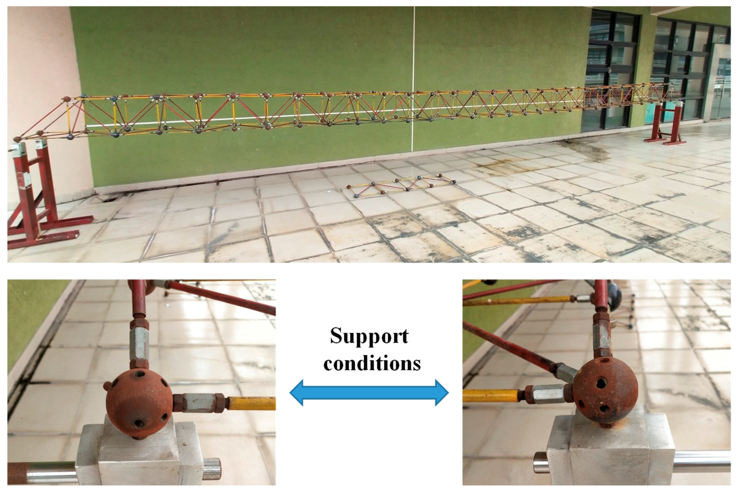
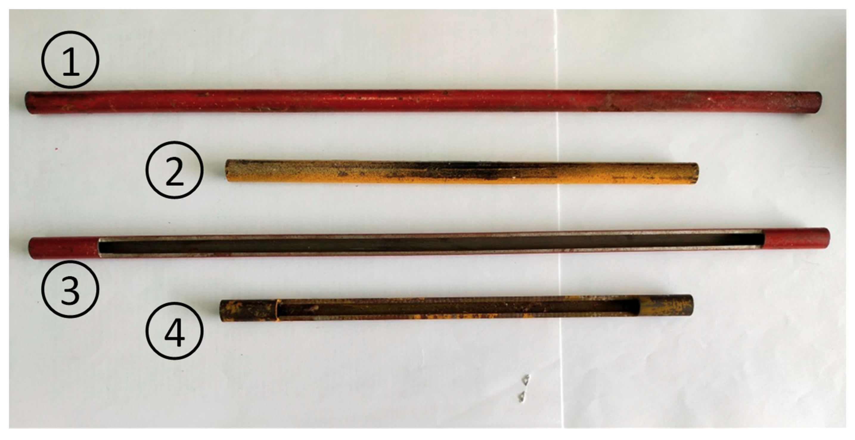
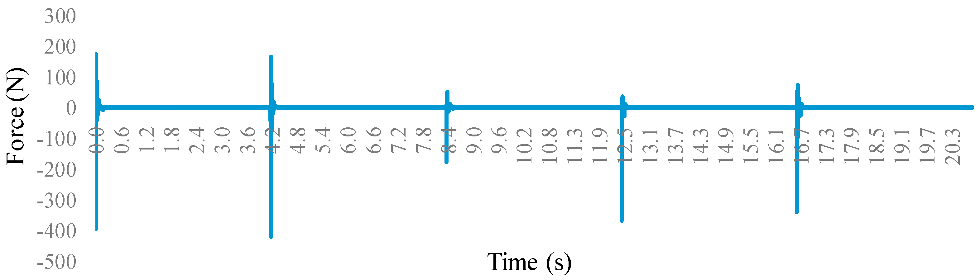
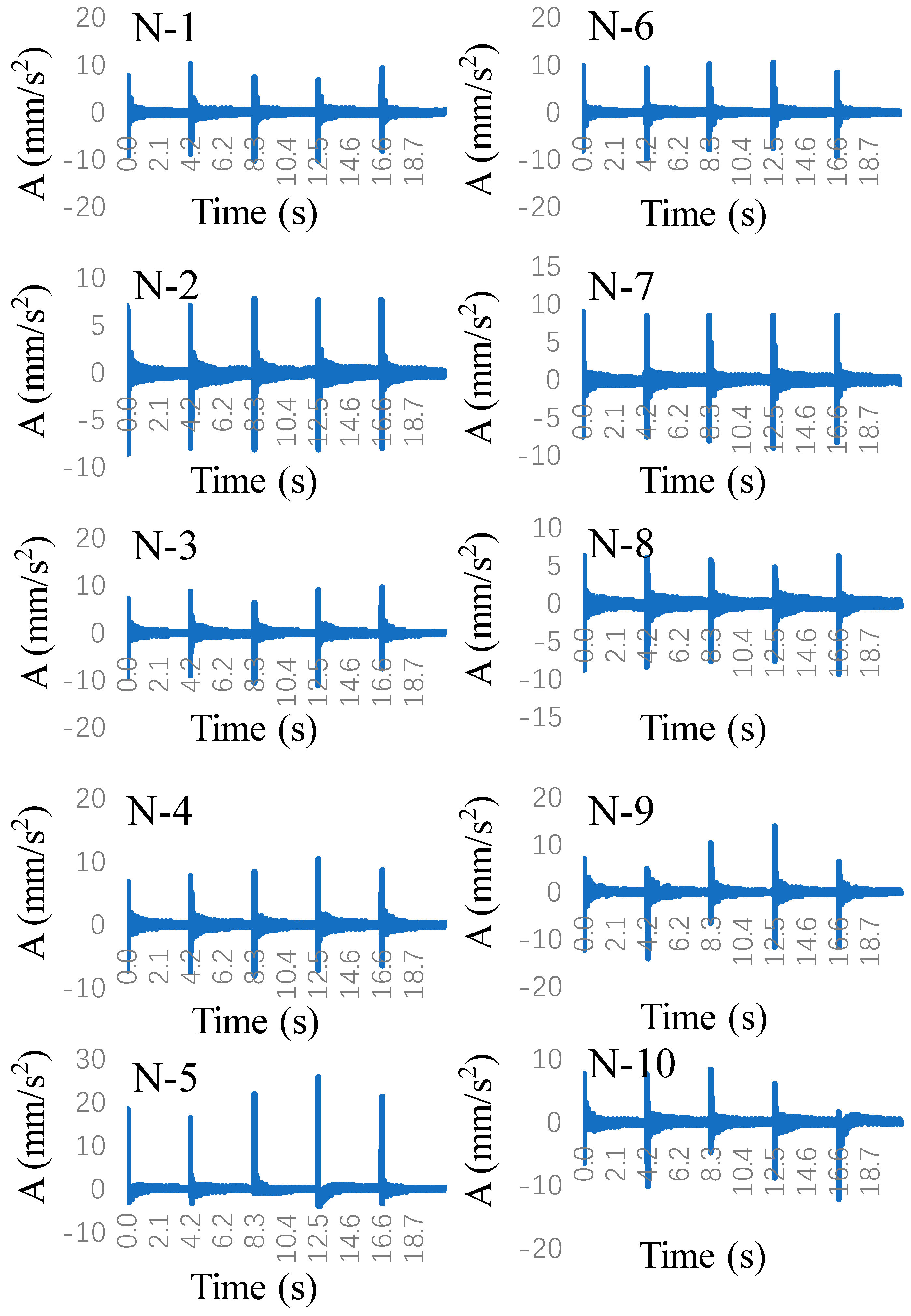
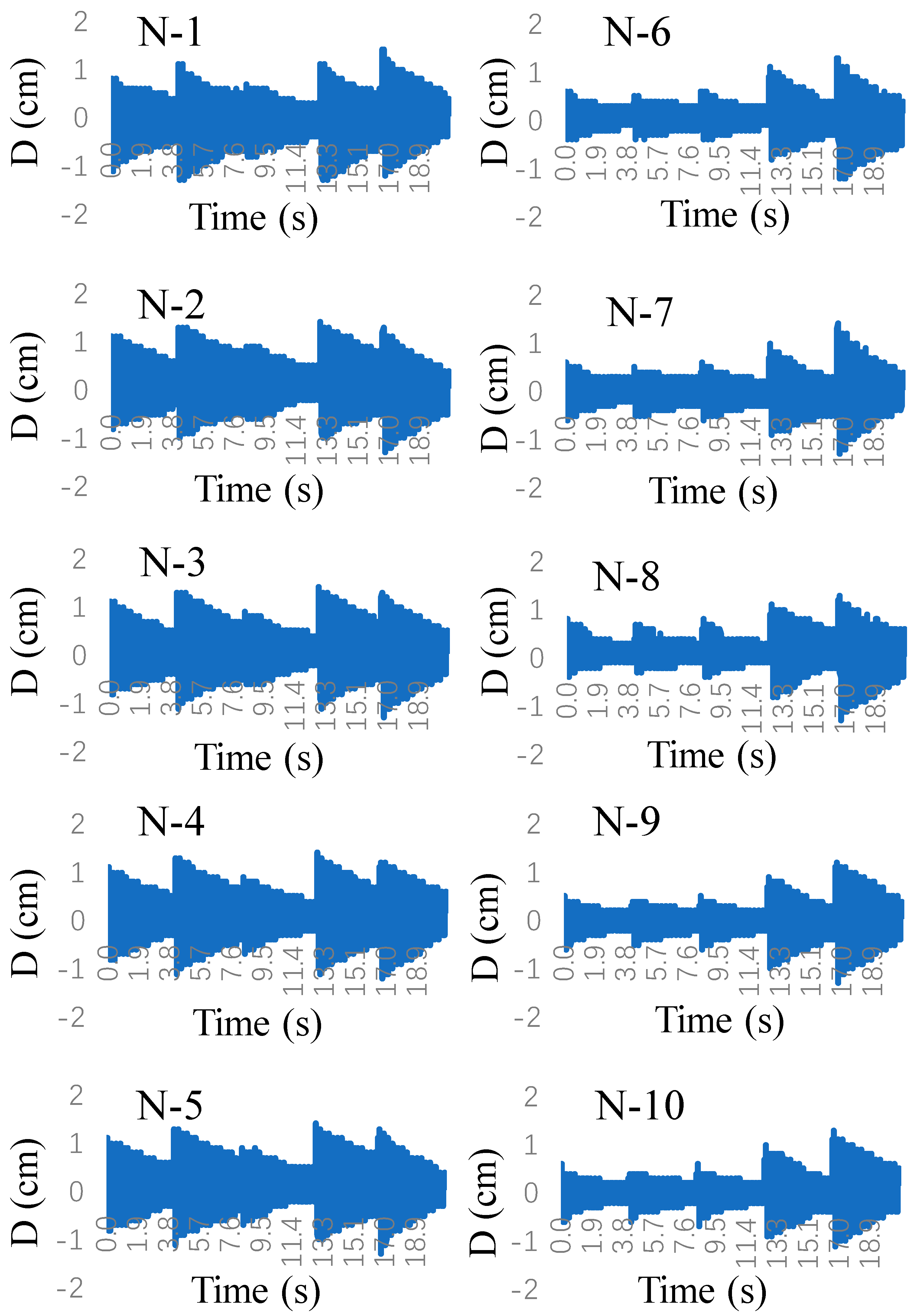
2.1. Vibration Experiment

A steel frame was used in this paper for the experiment (Figure 1); this beam consisted of 381 rods, and its length, width, and height were 10.62, 0.354, and 0.354 m, respectively. Each rod had a hollow circular cross section with an external radius of 0.005 m and thickness of 0.002 m. The rods were connected by steel balls. Vibration measurement methods (accelerometers and high-speed camera) were used to obtain the vibration signals. Experimental facilities (Figure 2) included: A FASTCAM SA3 high-speed camera, a JM3840 dynamic data acquisition instrument, 10 accelerometers, an instrumented hammer, and laptops. The weights of the structure, accelerometers and cables were 149.24, 0.52, and 0.84 kg, respectively; hence, the influence of the adding mass on the measurement results were negligible.
The vibration signals of the structure were collected by accelerometers (YD2150, Jing-Ming Technology Inc., Yangzhou, China) and a high-speed camera (FASTCAM SA3, Photron Inc., Tokyo, Japan), with a sampling frequency of 250 Hz. Vibration signals and force signals were processed by JMTST dynamic signal analysis software, and then modal analysis was carried out to obtain the experimental modal parameters (modal shapes and frequencies). Meanwhile, the high-speed camera recorded the frame pictures (8 bit) in the process of vibration, and the displacement signal of the structure could be obtained by using DIC (digital image correlation) skills. The principle of tracking the movement of points of interest using DIC [36,37] was expressed in the following formula:
C ( Δ x , Δ y ) = S I 0 ( x , y ) I 1 ( x + Δ x , y + Δ y ) d x d y S I 0 2 ( x , y ) d x d y · S I 1 2 ( x + Δ x , y + Δ y ) d x d y
where I 0 ( x , y ) and J ( x , y ) are the gray-scale distributions of two images, and the real displacement ( Δ x , Δ y ) of the reference subset (S) maximizes the function C ( Δ x , Δ y ) .
The accelerometers were installed on 10 nodes (Figure 3). The steel frame was excited 5 times with the hammer at the excitation point (the distances between the excitation point and the two supports were 3.894 and 6.726 m, respectively), the force signal was collected by the force sensor, and the accelerometers and the high-speed camera were used to collect the acceleration and displacement of the points of interest. The modal analysis was carried out by using JMTST dynamic signal analysis software, and the first-order frequency and modal shape were obtained. Then the first-order MSE of the structure was calculated (Equation (2)) [12].
M S E j = ϕ T K j ϕ
where ϕ and K j were the first-order modal shape and stiffness matrix of the j-th rod, respectively.
This paper mainly addressed 4 structural states. State (1): Intact structure; State (2): Damage on Rod 2; State (3): Damage on Rod 11; State (4): Simultaneous damage on Rod 2 and Rod 11. Damage was introduced by cutting off 50% of the cross section (in practical engineering, damage may be caused by corrosion, cracks and other reasons); the intact and damaged rods are shown in Figure 4. The damage index was the change rate of the modal strain energy (MSECR).
M S E C R = | M S E d a m a g e M S E i n t a c t | M S E i n t a c t
where the M S E d a m a g e and M S E i n t a c t are the modal strain energy of the damaged structure and intact structures.

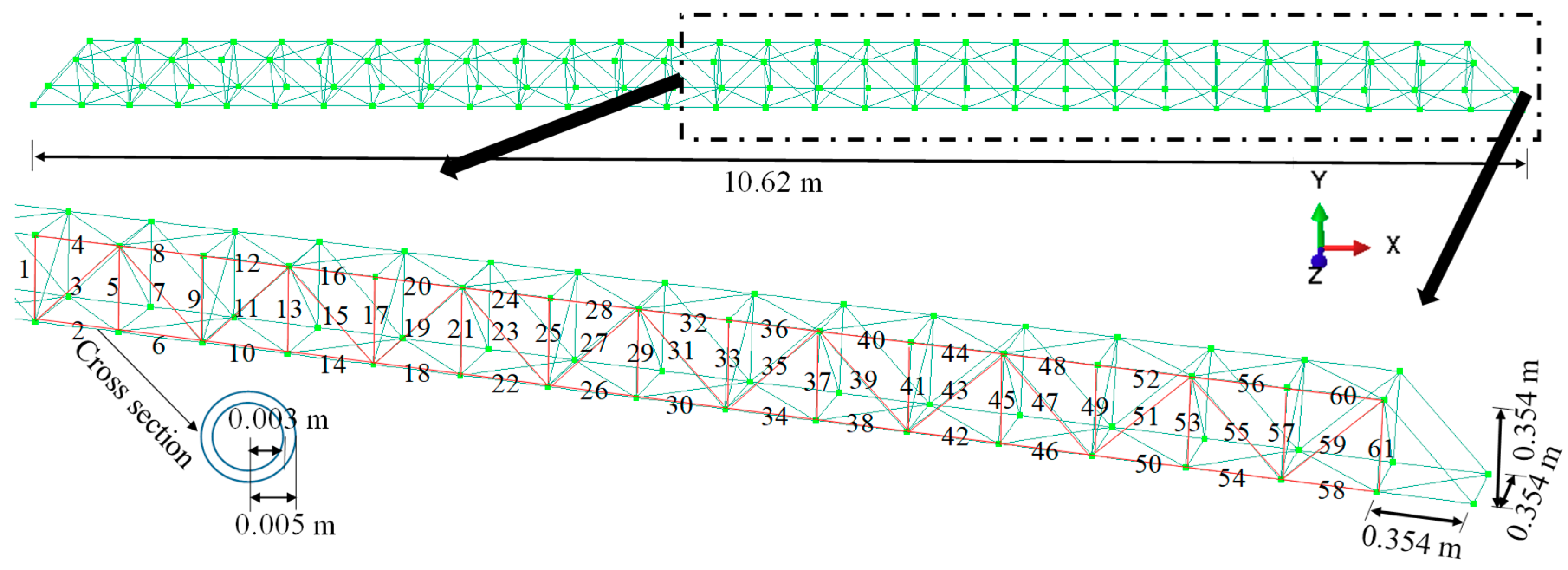
2.2. Numerical Simulation and CNN Samples

A numerical model of the steel frame (Figure 5) with a length of 10.62 m, a width of 0.354 m and a height of 0.354 m was developed by using the finite element software package ABAQUS (SIMULIA Inc., Providence, RI, USA). Each rod had a hollow circular cross section with a radius of 0.005 m and thickness of 0.002 m; additional weight (0.45 kg) was added at each node to simulate the steel ball of the real structure. The elastic modulus, Poisson’s ratio, density, and modal damping ratio were 212 GPa, 0.288, 7800 kg/m3, and 0.02, respectively. All rods were meshed with beam element (B31 type).
The performance of the structure could be changed by both damage in the elements and damage in the connections. A bridge case showed that the damage in the cables had greater effect on the structural characteristics than that in the connections [38]. In this paper, the damage of a rod was simulated by the change of its elastic modulus. It was assumed that the damage level of a rod was proportional to the reduction of its elastic modulus value. Only 1 level of damage was considered, i.e., the elastic modulus of the rod was reduced by 50%.
In this paper, the training samples of CNNs were derived from the numerical simulation data. Firstly, the single damage was studied, which means that the damage in one rod was considered for each damage scenario. The structure consisted of 61 rods (Figure 5); thus, there were 62 CNN samples including 61 damage scenarios plus the intact structure.
For the scenario with damage simultaneously in 2 rods, two of rods 1–17 were randomly selected; the damage level was 50%. There were 136 ( C 17 2 ) damage scenarios, i.e., 136 training samples.

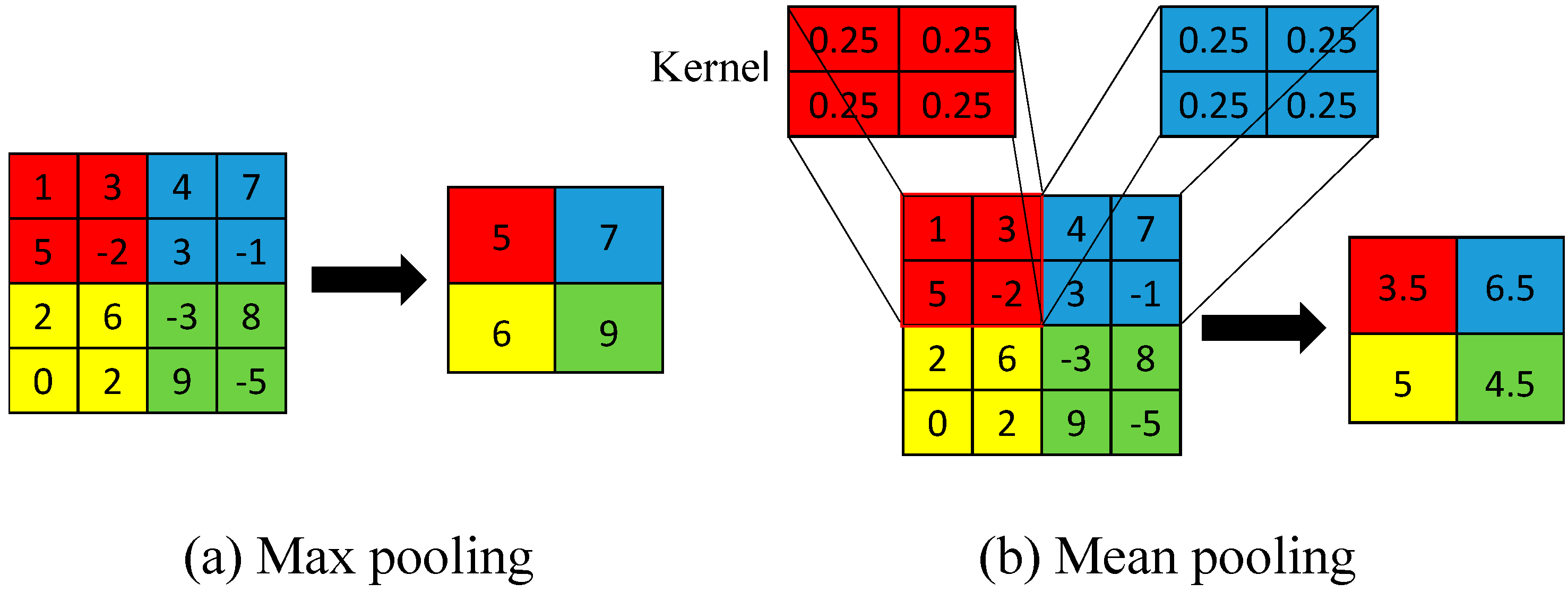
2.3. Convolutional Neural Network

The CNN was designed and trained using the Deep Learning Toolbox in MATLAB (MathWorks Inc, Natick, MA, USA). The network included one input layer, two convolution layers, one pooling layers, two activation layers, one fully connected layer, and one output layer (classification layer). For classification problems, one softmax layer was added after the fully connected layer. The explanations for the activation function and convolution and pooling processes are given in the Appendix A. The network architecture and structural parameters of the CNN are shown in Figure 6 and Table 1.

2.4. Input and Output of CNN Samples

The CNN input data of a single damage location, i.e., the MSECR of each rod (61 rods), was collected for each damage scenario, and 3 zeros were added, so the input consists of 64 (61 + 3) numbers; an 8 × 8 matrix was constructed as the input. In the testing stage, only the MSE of 17 rods was obtained from vibration experiment, so the missing data in the CNN input data were supplemented by numerical simulation data (i.e., the MSECR of Rods 18–61) [39]. This paper used a classification method to detect the single damage location, which was set to different categories, i.e., the intact condition was set to 0, the damage on the element 1 set to 1, the damage on the element 2 set to 2, and so on.
For multiple damage detection, each damage scenario was set to a category, i.e., the damage on the rods 1 and 2 set to 1, the damage on the rods 1 and 3 set to 2, the damage on the rods 1 and 17 set to 16, the damage on the rods 2 and 3 set to 15, and so on.
To realize the classification, the fully connected layer was followed by a softmax layer which used the softmax function to calculate a probability. The softmax function took the vector Z of K real numbers as its input and normalizes it into a vector ( z ) , the probability distribution of which consists of K probabilities. The function is defined by Equation (4).
σ ( z ) j = exp ( Z j ) k = 1 K exp ( Z k )
for j = 1, …, K and Z = ( Z 1 , , Z K ) K ; obviously 0 σ ( z ) 1 and j = 1 K σ ( z ) j = 1 . Applying this function to the CNN, the softmax function was used to solve a multi-classification problem. The predicted probability for the j-th class for a given sample vector x and a weighting vector w was:
P ( y = j | x ) = exp ( x T w j ) k = 1 K exp ( x T w k )
for j = 1, …, K, where 0 P ( y = j | x ) 1 and j = 1 K P ( y = j | x ) = 1 ; moreover, x was the output of the fully connected layer, w was the connection weights between the network outputs and target outputs, P ( y = j | x ) was the conditional probability of belonging to the j-th class, with x being the input.
A classification layer computed the cross entropy loss for multi-class classification problems with mutually exclusive classes. For typical classification networks, the classification layer must follow the softmax layer. The cross entropy was used to estimate the difference between the target damage location and the predicted damage location, and it is defined in Equation (6) [40].
L o s s = i = 1 N j = 1 K t i j ln y i j
In this paper, N was the number of the damage and intact cases, K was the number of damage location, t i j was the indicator that the i-th sample belongs to the j-th element (damage location), and y i j was the output for sample i for damage element j. Loss represented the difference between the predicted damage and the actual damage, and it was used to judge the training state (convergence or divergence) of the network.

3. Results

Based on the network trained by simulation data, the experimental data were inputted into the neural network to detect the structure state. The detection process was mainly divided into the following parts: (1) The modal parameters were obtained through modal analyses of vibration signals and force signals; (2) the experimental data were inputted into the CNN to detect the structure state; (3) the same method was applied to the BP neural network, and the detection results were compared.

3.1. Experimental Results

Figure 7 is the time-history curve of force (intact structure), and Figure 8 is the time-history curve of acceleration (1–10 nodes). Sampling time was 20.5 s.
Figure 9 is the displacement time-history curve of 10 nodes of the intact structure, which was obtained by the DIC method from 5120 pictures captured by the high-speed camera.
Vibration signals for other damage scenarios are shown in the Supplementary Document. The modal parameters of the structure were obtained by modal analysis of the collected excitation (force), acceleration and displacement signals. Table 2 and Table 3 are the first-order natural frequency of different structural states. Table 4 and Table 5 are the modal shape and rotation of different structural states, and the calculation of rotation was based on the formula [41]: θ i = ϕ ( x i ) , where x i was the location of the node i separating two adjacent elements, i = 1, 2, …, 10. The MSE (Equation (2)) was calculated. According to the MSE of the intact structure and the damaged structure, the MSECR (Equation (3)) was calculated. The MSECR obtained from the data of accelerometer and high-speed camera, respectively, and the results are shown in Appendix B (Table A1 and Table A2).

3.2. Structural Damage Detection

The numerical simulation data were used to train the network, and then the experimental data were used to verify the damage detection effect of the CNN on the real structure [39]. For the detection of single damage and intact structure, there were 62 training samples and six testing samples. For each structural state, the MSE of only 17 rods was obtained by experiment (the MSE of Rods 18–61 was obtained by finite element method), so the experimental data were incomplete. The finite element simulation data of Rods 18–61 were added as the input of the CNN (training with numerical simulation data). The data (accelerometer and high-speed camera) were inputted into the training network, and the experimental verification results are shown in Table 6.
Then, the experimental data (simultaneous damage at two locations) were detected by the classification algorithm. There were 136 training samples and two testing samples. The experimental data obtained from the simultaneous damage of Rods 2 and 11 (Section 2.4) showed that the target category was 25. The prediction results are shown in Table 7.
Table 6 and Table 7 illustrate that the CNN could correctly detect intact structure, single damage, and multiple damages.

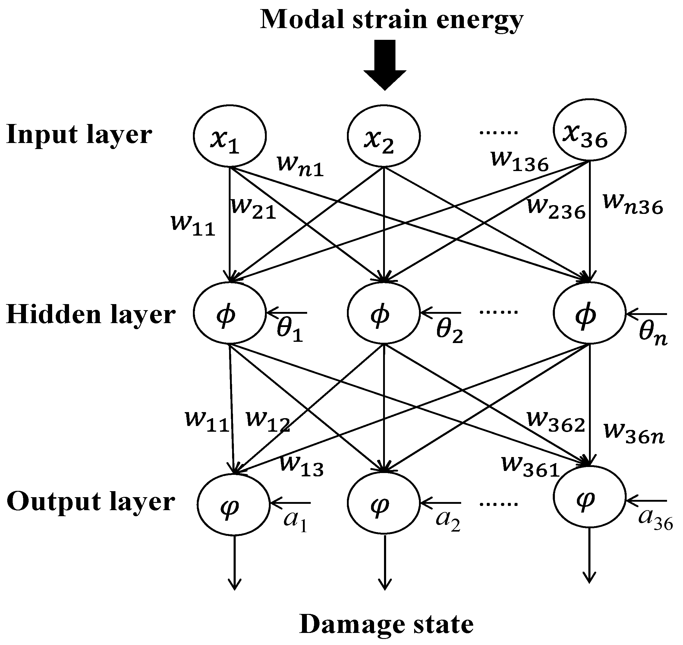
3.3. Damage Detection by BP Neural Network

Firstly, the BP neural network was trained with numerical simulation data, and then the experimental data were inputted into the network to detect the damage scenarios of the structure. The basic principle and topology of the BP neural network re in Appendix C. Table 8 and Table 9 are the damage detection results of BP neural network for the experimental data of accelerometers and high-speed camera, respectively.
Table 8 and Table 9 show that BP neural network could correctly detect single damage. However, the detections for intact structure and multiple damages were failed.

4. Discussion and Conclusions

It can be seen from Section 3.1 that the CNN was effective in detecting single damage and multiple damage. In this paper, the simulation data were used to train the network, and then the experimental data were applied to test the network, which achieved excellent detection results. In practical applications, it is usually difficult to get enough training samples for actual structures. This issue could will hinder the applications of ANNs in structural damage detection (especially for large structures). In this paper, it was overcome because the missing data of measurement were supplemented by simulation data; the CNN test results show that it was effective. The current study shows that CNNs could learn the damage features from finite element models firstly, and, thus, the damage of the real structure may be accurately predicted.
Compared with the BP neural network, the damage detection result of the CNN was better. The intact structure and damaged structures have different features, and different damage locations also show different features. In this paper, the feature of damaged structures was the MSECR. By comparing the damage detection results of Section 3.2 and Section 3.3, it was found that the BP neural network was effective for detecting a single damage location, but it was inaccurate in detecting multi-damage and intact structure. Nevertheless, these features (intact structure, single damage, and multi-damage) can be extracted by the CNN.
In this paper, the reduction of elastic modulus does not represent all real damage cases in engineering structures. Other damages, e.g., corrosion, cracks, and degradation, may also induce changes in mechanical parameters. Therefore, it is necessary to combine other technologies (e.g., image recognition to detect the surface of structures) for comprehensive damage detection in real structures.
Based on the above discussion, the following conclusions are drawn:
  • As a classifier, the CNN can accurately detect structural damage.
  • The CNN was more effective than the BP neural network in damage detection.
  • The experimental verifications proved that the CNN can be trained by simulation data and applied to measured data.
  • It was feasible to supplement the missing data of the experiment with the simulated data in the CNN input.

Supplementary Materials

They are available online at https://www.mdpi.com/2076-3417/9/16/3376/s1.

Author Contributions

S.T. contributed to the paper in conceptualization, methodology, investigation, formal analysis, original draft preparation, software, visualization, and data curation. G.C. contributed to the paper in conceptualization, methodology, investigation, formal analysis, original draft preparation, and supervision. G.L. and J.L. contributed to the paper in investigation, formal analysis, and review and editing. F.C. contributed to the paper in conceptualization, methodology, original draft preparation, and review and editing.

Funding

This research received no external funding.

Conflicts of Interest

The authors declare no conflicts of interest.

Appendix A

The convolution process (Figure A1) is to multiply each element in the convolution kernel (red matrix) with the corresponding element in a sub-region (yellow part) of the input data of the convolution layer and sum up the products to obtain an element in the feature matrix (green part). Each time, the sub-region moves either down or right at a step size, and the process is repeated until all elements of the input data are involved; in the end, the convolution operation form a new matrix (i.e., the feature matrix).
Figure A1. Convolution process.
Applsci 09 03376 g0a1
The pooling layer is used to reduce the dimensions of the input matrix. There are usually two different pooling methods: max pooling (Figure A2a) and mean pooling (Figure A2b). Max pooling was used in this paper because it is better than mean pooling [42]. As shown in Figure A1a, max pooling picks up the maximum value of a sub-matrix (2 × 2) to form an element of the feature matrix.
Figure A2. Pooling process.
Applsci 09 03376 g0a2
Activation function: A leaky rectified linear unit (ReLU) function performs a threshold operation where any input value less than zero is multiplied by a fixed scalar. This operation is equivalent to:
f ( x ) = { x , x 0 s c a l e x ,    x < 0

Appendix B

Table A1. The change rate of the modal strain energy (MSECR) under each case based on accelerometers.
RodState (2)State (3)State (4)
10.1832610.1331590.750995
210.5611221
30.1223370.0521170.232933
40.0105880.0689080.006570
50.0116350.0047790.026812
60.0106110.0823430.036997
70.0047570.0516240.012947
80.0023400.0513310.005684
90.0087310.0003860.004622
100.0051280.0734520.003947
110.00788910.176934
120.0124250.1364640.003921
130.0100720.0934220.001367
140.0066580.325540.009835
150.0092210.0548080.003069
160.0113060.043270.00168
170.0048890.0089270.002931
Table A2. The MSECR under each case based on high speed camera.
RodState (2)State (3)State (4)
10.0015670.1024160.023301
210.0571570.252800
30.8629050.2322900.070087
40.0578930.2259770.101593
50.0703840.0146681
60.5796810.0584790.017674
70.0801070.0345380.089115
80.4348590.6942000.005681
90.0939820.3430200.209198
100.1202540.0677070.001401
110.05238710.632459
120.0744420.1089210.038028
130.1200960.1278490.100525
140.0809860.0891650.027459
150.0818810.1876160.015737
160.1257190.4544980.020225
170.1360110.3128100.011164

Appendix C

The topology of the BP neural network included an input layer, a hidden layer, and an output layer, as shown in Figure A3. In Figure A3, x 1 x 36 were the input (modal strain energy) and w k j and θ k were the weight and threshold of the k-th node of the hidden layer to the input layer, respectively, where k = 1, 2, …, n and j = 1, 2, …, 36; ϕ was the transfer function ( tan sig ( s ) = 2 / ( 1 + e x p ( 2 × s ) ) 1 ), where s was the input of the node) of the hidden layer. w i n and were the weight and threshold of the i-th node of the output layer to the hidden layer, respectively, where i = 1, 2, …, 36. The Levenberg–Marquardt (LM) algorithm [43] was used to adjust the weights and thresholds of the network to minimize the network error.
Figure A3. Topology of the back propagation (BP) neural network.
Applsci 09 03376 g0a3
As shown in Figure A3, the input of the hidden layer u i was as follows:
u i = i = 1 36 w i j x j + θ i
According to the transfer function of the hidden layer, the output of the i-th node of the hidden layer can be expressed as follows:
y i = ϕ ( u i ) = ϕ ( i = 1 36 w i j x j + θ i )
Therefore, the input of the output layer vi was as follows:
v i = i = 1 n w i n y i + a i = i = 1 n w i n ϕ ( i = 1 36 w i j x j + θ i ) + a i
According to Equations (A2)–(A4), the output of the output layer O was as follows:
O = φ ( v ) = φ ( i = 1 n w i n y i + a i ) = φ ( i = 1 n w i n ϕ ( i = 1 36 w i j x j + θ i ) + a i )
Assuming that the expected output of the output layer was T, the output error E was as follows:
E = i = 1 N ( T O ) 2
where N was the number of samples.
The training process of neural networks was the weights, and thresholds were constantly adjusted. Training terminated when the error does not change or was less than a certain value.

References

  1. Khatir, S.; Abdel Wahab, M. A computational approach for crack identification in plate structures using XFEM, XIGA, PSO and Jaya algorithm. Theor. Appl. Fract. Mech. 2019, 103, 102240. [Google Scholar] [CrossRef]
  2. Cha, Y.; Buyukozturk, O. Structural Damage Detection Using Modal Strain Energy and Hybrid Multiobjective Optimization. Comput. Aided Civ. Infrastruct. Eng. 2015, 30, 347–358. [Google Scholar] [CrossRef]
  3. Graybeal, B.A.; Phares, B.M.; Rolander, D.D.; Moore, M.; Washer, G. Visual Inspection of Highway Bridges. J. Nondestruct. Eval. 2002, 21, 67–83. [Google Scholar] [CrossRef]
  4. Hu, H.; Wu, C. Development of scanning damage index for the damage detection of plate structures using modal strain energy method. Mech. Syst. Signal Process. 2009, 23, 274–287. [Google Scholar] [CrossRef]
  5. Doebling, S.; Farrar, C.; Prime, M. A Summary Review of Vibration-Based Damage Identification Methods. Shock. Vib. Dig. 1998, 30, 91–105. [Google Scholar] [CrossRef] [Green Version]
  6. Khatir, S.; Tiachacht, S.; Le Thanh, C.; Khatir, T.; Capozucca, R.; Abdel Wahab, M. Damage Detection in Laminated Composite Plates Based on Local Frequency Change Ratio Indicator. In Proceedings of the 13th International Conference on Damage Assessment of Structures, Porto, Portugal, 9–10 July 2019; pp. 887–898. [Google Scholar]
  7. Cawley, P.; Adams, R.D. A Vibration Technique for Non-Destructive Testing of Fibre Composite Structures. J. Compos. Mater. 1979, 13, 161–175. [Google Scholar] [CrossRef]
  8. Cawley, P.; Adams, R.D. The location of defects in structures from measurements of natural frequencies. J. Strain Anal. Eng. Des. 1979, 14, 49–57. [Google Scholar] [CrossRef]
  9. Shen, M.H.H.; Grady, J.E. Free vibrations of delaminated beams. Aiaa J. 1992, 30, 1361–1370. [Google Scholar] [CrossRef] [Green Version]
  10. Pandey, A.K.; Biswas, M.; Samman, M.M. Damage detection from changes in curvature mode shapes. J. Sound Vib. 1991, 145, 321–332. [Google Scholar] [CrossRef]
  11. Zou, Y.; Tong, L.; Steven, G.P. Vibration-based model-dependent damage (delamination) identification and health monitoring for composite structures—A review. J. Sound Vib. 2017, 10, 165–193. [Google Scholar] [CrossRef]
  12. Shi, Z.Y.; Law, S.S.; Zhang, L.M. Structural damage localization from modal strain energy change. J. Eng. Mech. 2000, 218, 1216–1223. [Google Scholar] [CrossRef]
  13. Seyedpoor, S.M. A two stage method for structural damage detection using a modal strain energy based index and particle swarm optimization. Int. J. Non-Linear Mech. 2012, 47, 1–8. [Google Scholar] [CrossRef]
  14. Pal, J.; Banerjee, S. A combined modal strain energy and particle swarm optimization for health monitoring of structures. J. Civ. Struct. Health Monit. 2015, 5, 353–363. [Google Scholar] [CrossRef]
  15. Khatir, S.; Abdel Wahab, M.; Boutchicha, D.; Khatir, T. Structural health monitoring using modal strain energy damage indicator coupled with teaching-learning-based optimization algorithm and isogoemetric analysis. J. Sound Vib. 2019, 448, 230–246. [Google Scholar] [CrossRef]
  16. Kaveh, A.; Zolghadr, A. Cyclical Parthenogenesis Algorithm for guided modal strain energy based structural damage detection. Appl. Soft Comput. 2017, 57, 250–264. [Google Scholar] [CrossRef]
  17. Tran-Ngoc, H.; Khatir, S.; Roeck, G.D.; Bui-Tien, T.; Nguyen-Ngoc, L. Model Updating for Nam O Bridge Using Particle Swarm Optimization Algorithm and Genetic Algorithm. Sensors 2018, 18, 4131. [Google Scholar] [CrossRef] [PubMed]
  18. Guresen, E.; Kayakutlu, G. Definition of artificial neural networks with comparison to other networks. Procedia Comput. Sci. 2011, 3, 426–433. [Google Scholar] [CrossRef] [Green Version]
  19. Salehi, H.; Das, S.; Chakrabartty, S.; Biswas, S.; Burgueño, R. Structural damage identification using image-based pattern recognition on event-based binary data generated from self-powered sensor networks. Struct. Control Health Monit. 2018, 25, e2135. [Google Scholar] [CrossRef]
  20. Xu, H.; Humar, J.M. Damage Detection in a Girder Bridge by Artificial Neural Network Technique. Comput. Aided Civ. Infrastruct. Eng. 2010, 21, 450–464. [Google Scholar] [CrossRef]
  21. Yao, X. Evolutionary Artificial Neural Networks. Int. J. Neural Syst. 1993, 4, 203–222. [Google Scholar] [CrossRef]
  22. Yao, W.S. The Researching Overview of Evolutionary Neural Networks. Comput. Sci. 2004, 31, 125–129. [Google Scholar]
  23. Lin, Y.Z.; Nie, Z.H.; Ma, H.W. Structural Damage Detection with Automatic Feature extraction through Deep Learning. Comput. Aided Civ. Infrastruct. Eng. 2017, 32, 1–22. [Google Scholar] [CrossRef]
  24. Yuan, Z.W.; Zhang, J. Feature extraction and image retrieval based on AlexNet. In Proceedings of the Eighth International Conference on Digital Image Processing, Chengu, China, 29 August 2016. [Google Scholar]
  25. Krizhevsky, A.; Hinton, G. Learning multiple layers of features from tiny images. Tech. Rep. Univ. Tor. 2009, 1, 7. [Google Scholar]
  26. Lawrence, S.; Giles, C.L.; Tsoi, A.C.; Back, A.D. Face recognition: A convolutional neural-network approach. IEEE Trans. Neural Netw. 1997, 8, 98–113. [Google Scholar] [CrossRef] [PubMed]
  27. Tensmeyer, C.; Saunders, D.; Martinez, T. Convolutional Neural Networks for Font Classification. In Proceedings of the International Conference on Document Analysis and Recognition, Kyoto, Japan, 9–15 November 2017; pp. 985–990. [Google Scholar]
  28. Yao, D.; Zhu, W.; Chen, Y.; Zhang, L. Chinese license plate character recognition based on convolution neural network. In Proceedings of the Chinese Automation Congress, Jinan, China, 20–22 October 2017. [Google Scholar]
  29. Cha, Y.; Choi, W.; Büyüköztürk, O. Deep Learning-Based Crack Damage Detection Using Convolutional Neural Networks. Comput. Aided Civ. Infrastruct. Eng. 2017, 32, 361–378. [Google Scholar] [CrossRef]
  30. Li, R.; Yuan, Y.; Wei, Z.; Yuan, Y. Unified Vision-Based Methodology for Simultaneous Concrete Defect Detection and Geolocalization. Comput. Aided Civ. Infrastruct. Eng. 2018, 33, 527–544. [Google Scholar] [CrossRef]
  31. Zhang, Y.; Miyamori, Y.; Mikami, S.; Saito, T. Vibration-based structural state identification by a 1-dimensional convolutional neural network. Comput. Aided Civ. Infrastruct. Eng. 2019, 34, 1–18. [Google Scholar] [CrossRef]
  32. Tang, Z.; Chen, Z.; Bao, Y.; Li, H. Convolutional neural network-based data anomaly detection method using multiple information for structural health monitoring. Struct. Control Health Monit. 2019, 26, e2296. [Google Scholar] [CrossRef]
  33. Abdeljaber, O.; Avci, O.; Kiranyaz, M.S.; Boashash, B.; Sodano, H.; Inman, D.J. 1-D CNNs for structural damage detection: Verification on a structural health monitoring benchmark data. Neurocomputing 2018, 275, 1308–1317. [Google Scholar] [CrossRef]
  34. Abdeljaber, O.; Avci, O.; Kiranyaz, S.; Gabbouj, M.; Inman, D.J. Real-time vibration-based structural damage detection using one-dimensional convolutional neural networks. J. Sound Vib. 2017, 388, 154–170. [Google Scholar] [CrossRef]
  35. Kiranyaz, S.; Avci, O.; Abdeljaber, O.; Ince, T.; Gabbouj, M.; Inman, D.J. 1D Convolutional Neural Networks and Applications: A Survey. arXiv 2019, arXiv:1905.03554. [Google Scholar]
  36. Chu, T.C.; Ranson, W.F.; Sutton, M.A. Applications of digital-image-correlation techniques to experimental mechanics. Exp. Mech. 1985, 25, 232–244. [Google Scholar] [CrossRef]
  37. Pan, B.; Qian, K.; Xie, H.; Asundi, A. Two-dimensional digital image correlation for in-plane displacement and strain measurement: A review. Meas. Sci. Technol. 2009, 20, 152–154. [Google Scholar] [CrossRef]
  38. Bedon, C.; Dilena, M.; Morassi, A. Ambient vibration testing and structural identification of a cable-stayed bridge. Meccanica 2016, 51, 2777–2796. [Google Scholar] [CrossRef] [Green Version]
  39. Lee, J.J.; Lee, J.W.; Yi, J.H.; Yun, C.B.; Jung, H.Y. Neural networks-based damage detection for bridges considering errors in baseline finite element models. J. Sound Vib. 2005, 280, 555–578. [Google Scholar] [CrossRef]
  40. Bishop, C.M. Pattern Recognition and Machine Learning (Information Science and Statistics); Springer: New York, NY, USA, 2007. [Google Scholar]
  41. Guan, H.; Karbhari, V.M. Improved damage detection method based on Element Modal Strain Damage Index using sparse measurement. J. Sound Vib. 2008, 309, 465–494. [Google Scholar] [CrossRef]
  42. Scherer, D.; Müller, A.; Behnke, S. Evaluation of Pooling Operations in Convolutional Architectures for Object Recognition. In Proceedings of the International Conference on Artificial Neural Networks, Berlin, Germany, 17–19 September 2010. [Google Scholar]
  43. Geng, X.; Lu, S. Researchon FBG-Based CFRP Structural Damage Identification Using BP Neural Network. Photonic Sens. 2018, 8, 168–175. [Google Scholar] [CrossRef]
Figure 1. The steel frame modal with 381 rods.
Applsci 09 03376 g001
Figure 2. Experimental facilities. (a) accelerometers; (b) hammer; (c) JM3840 dynamic data acquisition instrument; (d) FASTCAM SA3 high-speed camera; (e) laptop.
Applsci 09 03376 g002
Figure 3. Location of excitation point and accelerometers. N-#: Installation point of accelerometers; R-#: Rods 1–17.
Applsci 09 03376 g003
Figure 4. Intact rod (Rods 1 and 2) and damaged rod (Rods 3 and 4, with 50% cut-off of the cross section).
Applsci 09 03376 g004
Figure 5. Numerical model of the steel frame with 381 rods.
Applsci 09 03376 g005
Figure 6. Convolutional neural network (CNN) framework. C1, C2: Convolution layer; P: Pooling layer; FC: Fully connected layer.
Applsci 09 03376 g006
Figure 7. The time-history curve of force.
Applsci 09 03376 g007
Figure 8. The time-history curve of acceleration. A: Acceleration.
Applsci 09 03376 g008
Figure 9. The time-history curve of displacement. D: Displacement.
Applsci 09 03376 g009
Table 1. Structural parameters of the CNN.
LayerTypeKernel Num.Kernel SizeStridePadActivation
1InputNoneNoneNoneNoneNone
2Convolution (C1)2003 × 3[1,1]0Leaky ReLU
3Max pooling (P)None2 × 2[1,1]0None
4Convolution (C2)4002 × 2[1,1]0Leaky ReLU
5FCNoneNoneNoneNoneNone
6SoftmaxNoneNoneNoneNoneNone
7ClassificationNoneNoneNoneNoneNone
Table 2. Natural frequency of steel frame structure based on accelerometer.
Structure StateFirst-Order Natural Frequency (Hz)
state (1)3.906
state (2)3.906
state (3)3.906
state (4)3.662
Table 3. Natural frequency of steel frame structure based on high speed camera.
Structure StateFirst-Order Natural Frequency (Hz)
State (1)3.906
State (2)3.906
State (3)3.906
State (4)3.906
Table 4. The first-order modal shape based on accelerometer.
NodeState (1)State (2)State (3)State (4)
Modal ShapeRotationModal ShapeRotationModal ShapeRotationModal ShapeRotation
10.645−0.00070.0580.00600.655−0.00170.2750.0066
20.6410.00010.105−0.00020.627−0.00020.401−0.0009
30.624−0.00150.080−0.00180.625−0.00010.298−0.0022
40.551−0.00200.055−0.00100.606−0.00110.234−0.0005
50.5350.00180.043−0.00030.537−0.00310.2410.0007
60.6150.00330.193−0.00390.5990.00060.570−0.0035
70.6650.00020.105−0.00110.6510.00100.357−0.0006
80.646−0.00110.089−0.00010.649−0.00160.309−0.0007
90.606−0.00150.081−0.00030.524−0.00230.180−0.0009
100.558−0.00160.062−0.00070.5440.00420.2610.0020
Table 5. The first-order modal shape based on high-speed camera.
NodeState (1)State (2)State (3)State (4)
Modal ShapeRotationModal ShapeRotationModal ShapeRotationModal ShapeRotation
10.3210.00210.044−0.00730.2280.00200.2640.0036
20.3280.00030.0370.00230.2540.00050.2910.0003
30.324−0.00170.0480.00160.243−0.00170.279−0.0018
40.312−0.00190.046−0.00160.199−0.00200.250−0.0017
50.3100.00180.0440.00160.1930.00210.2450.0016
60.3190.00650.0390.00860.2190.00550.2410.0035
70.3380.00070.045−0.00100.243−0.00060.2590.0003
80.333−0.00190.041−0.00200.224−0.00190.251−0.0018
90.323−0.00130.0400.00040.209−0.00080.231−0.0017
100.3240.00210.0410.00030.204−0.00120.2280.0017
Table 6. Experimental verification results for single damage scenarios and intact structure.
Testing DataActual LocationPredicted LocationProbability
A-10 (Intact)0 (Intact)76.7%
A-22263.8%
A-3111197.8%
H-10 (Intact)0 (Intact)99.6%
H-22299.7%
H-3111186.9%
Note: A-#: Accelerometer measurement; H-#: High-speed camera measurement.
Table 7. Experimental verification results for multi-damage.
Testing DataActual CategoryPredicted CategoryProbability
A-M2525100%
H-M252599.9%
Note: A-M: Accelerometer measurement; H-M: High-speed camera measurement.
Table 8. Damage detection results of experimental data (accelerometers).
Number of Hidden Layer NodesActual Damage States
(1)(2)(3)(4)
55282111 and 5
60152111 and 15
65132111 and 5
70132111 and 5
Note: 0 was intact structure; 2 was damage on Rod 2; and so on.
Table 9. Damage detection results of experimental data (high-speed camera).
Number of Hidden Layer NodesActual Damage States
(1)(2)(3)(4)
5512111 and 5
6012111 and 5
6512111 and 5
7012111 and 5

