Space Syntax Analysis Applied to Urban Street Lighting: Relations between Spatial Properties and Lighting Levels

 ,
, 
 ,
, 

Abstract
:1. Introduction
Research Scope
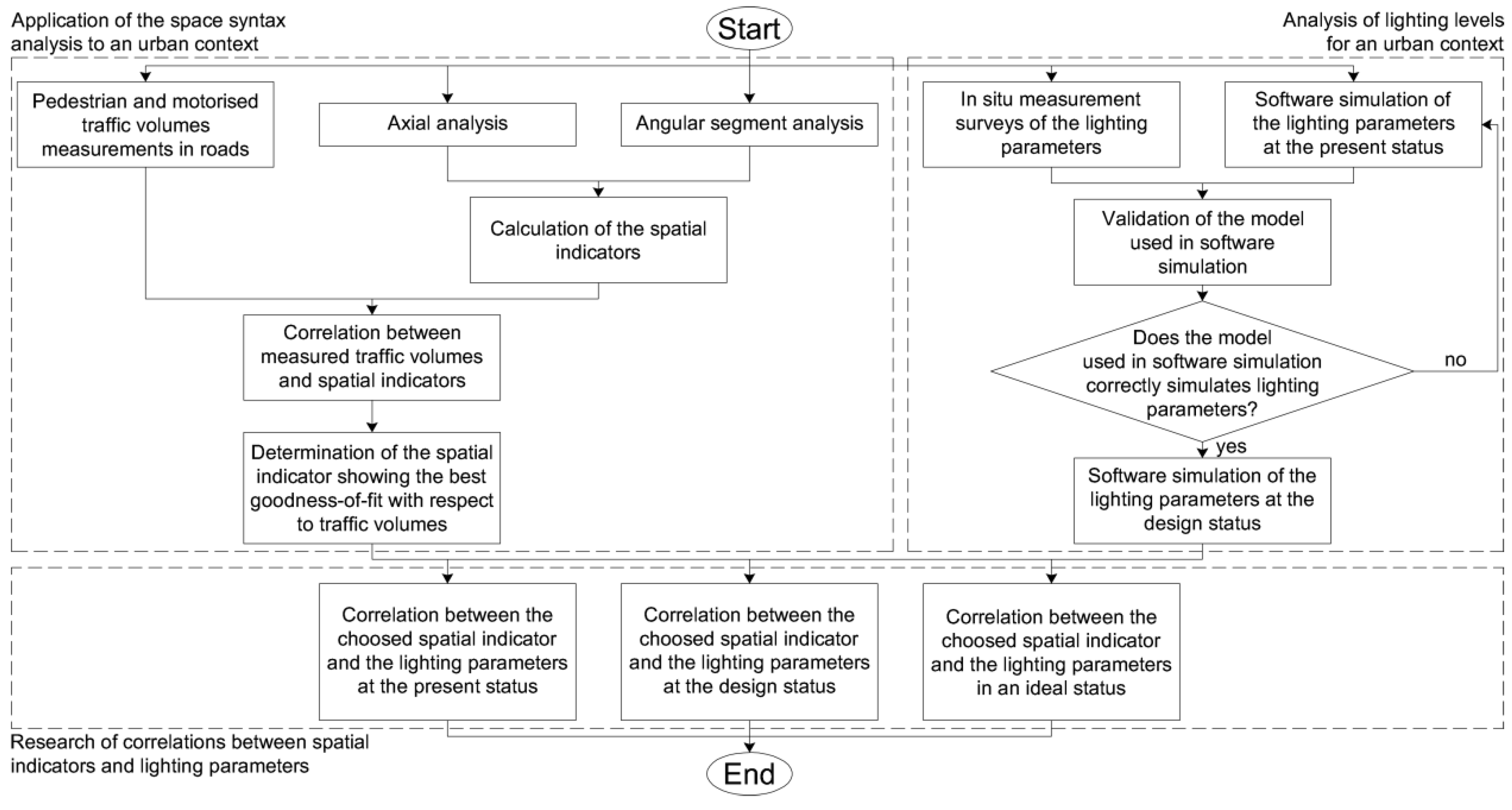
2. Application of the Space Syntax Analysis to an Urban Context
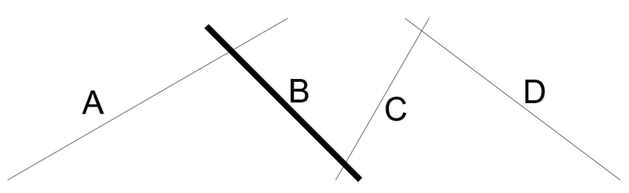
2.1. Space Syntax Analysis Theoretical Concepts
2.2. Spatial Indicators Assessment
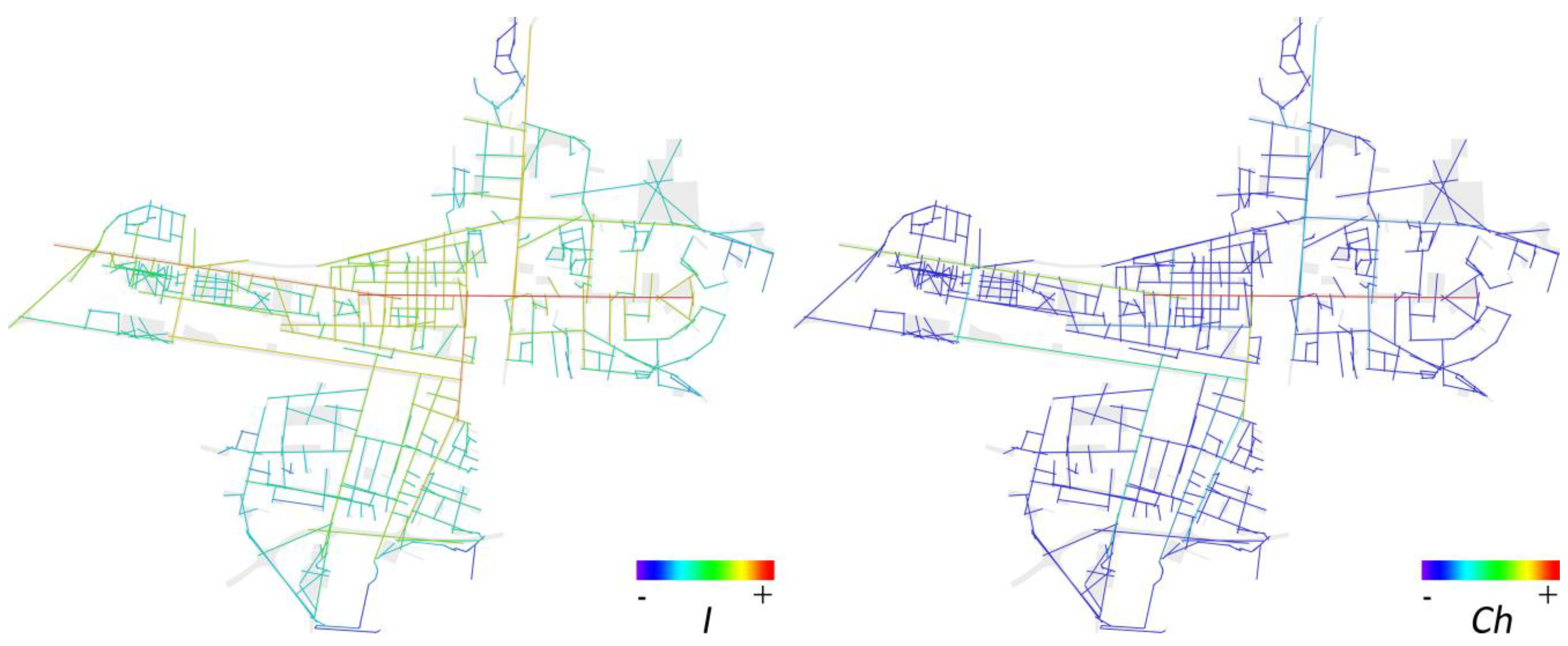
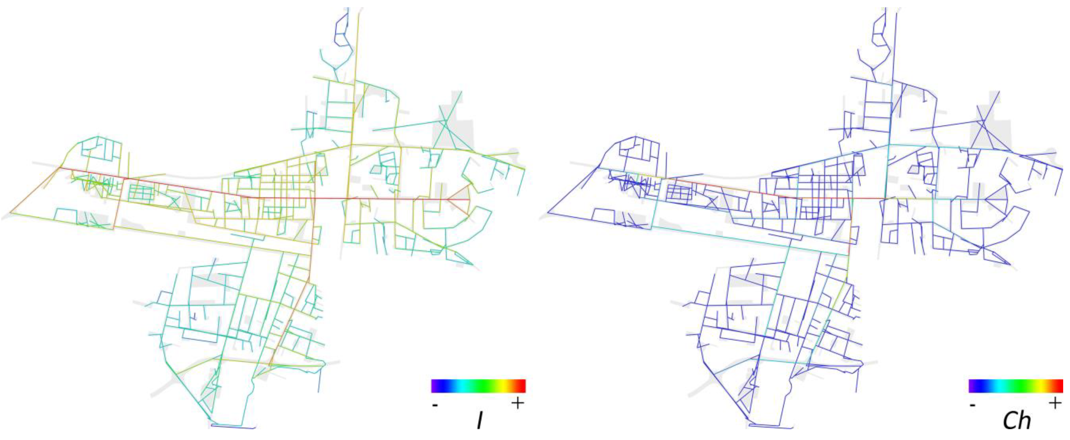
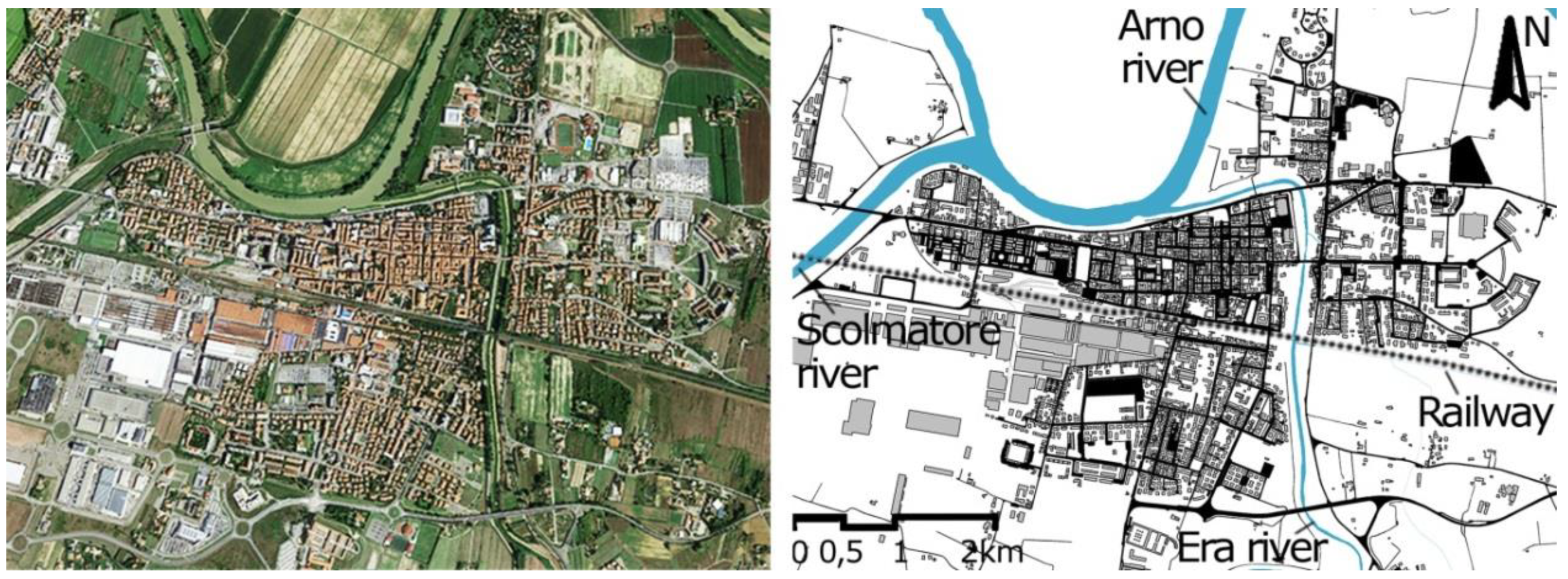
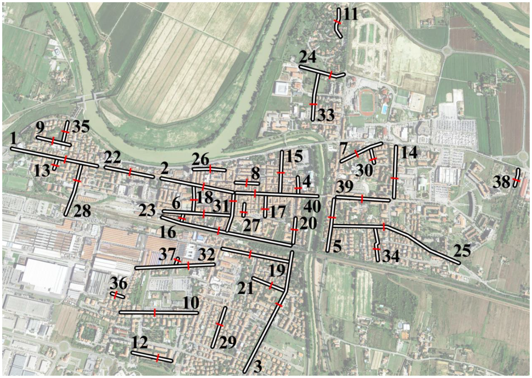
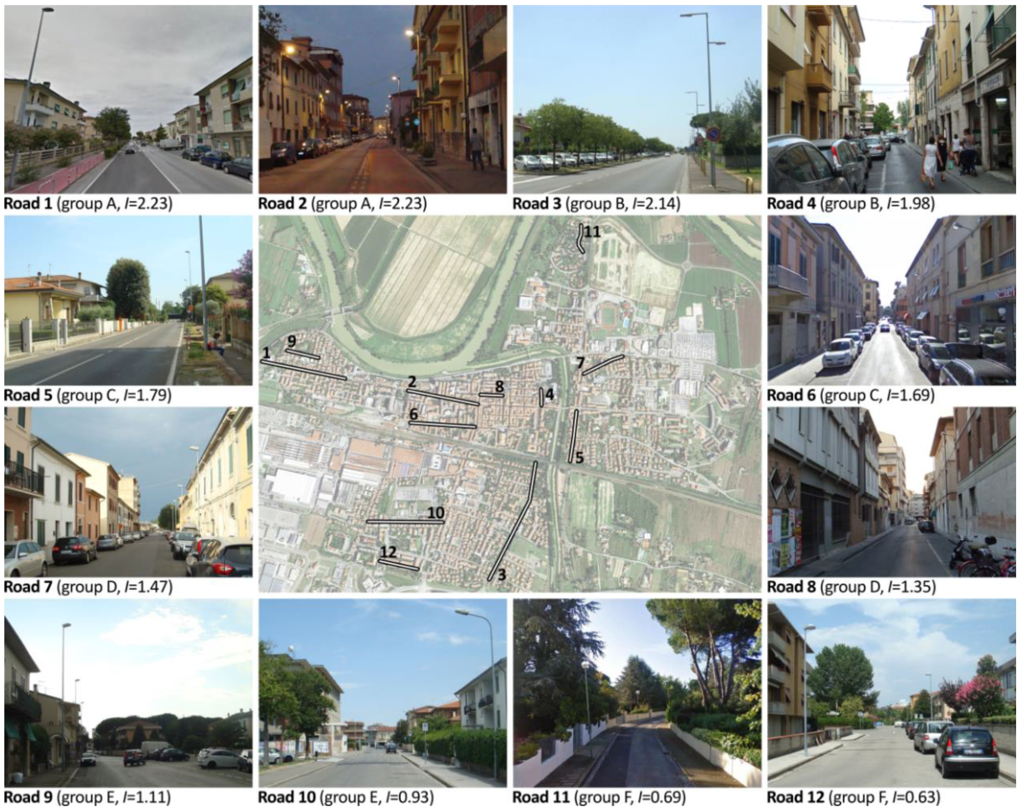
2.3. Space Syntax Analysis of Pontedera Urban Context
2.4. Observation Campaign of Pedestrian and Motorised Traffic
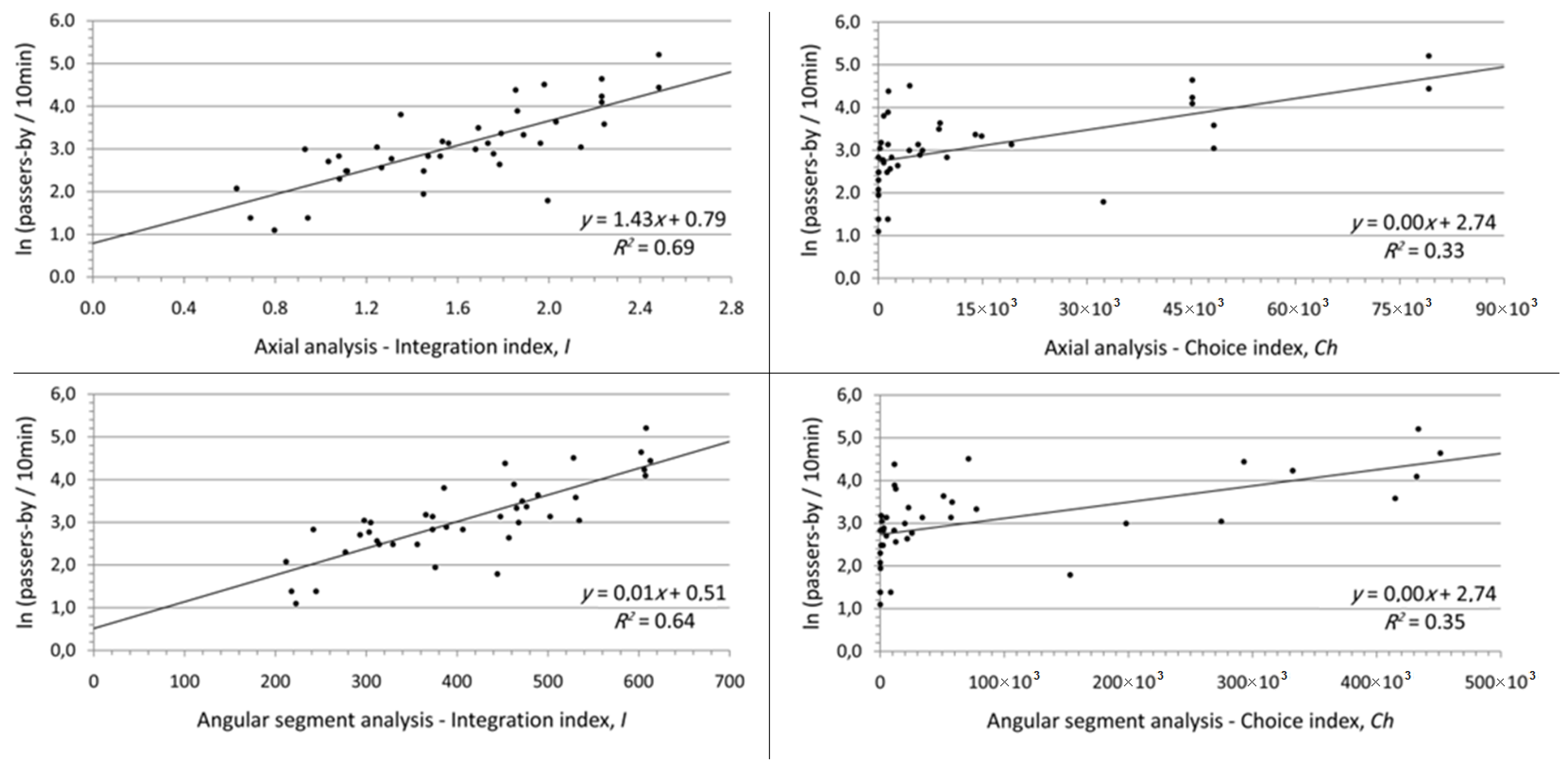
2.5. Correlations between Traffic Volumes and Spatial Indicators
3. Analysis of the Lighting Levels for an Urban Context
3.1. In Situ Measurements of the Lighting Parameters
3.2. Software Simulations of the Lighting Parameters at the Present Status and Validation of the Model
3.3. Software Simulation of the Lighting Parameters at the Design Status and Refurbishment Project
4. Correlations between Spatial Indicators and Lighting Parameters
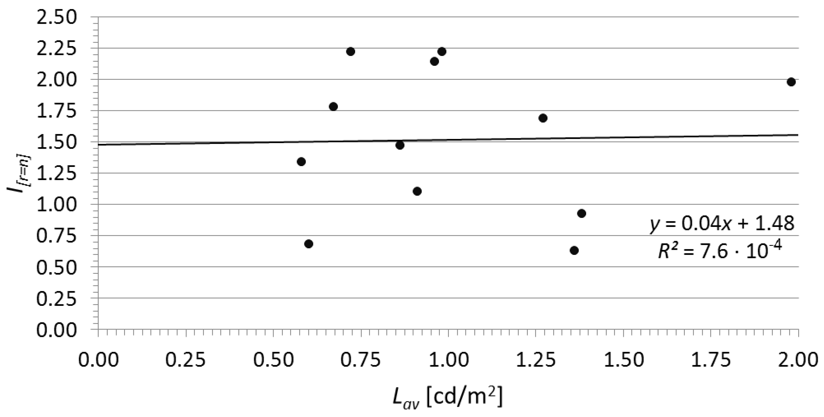
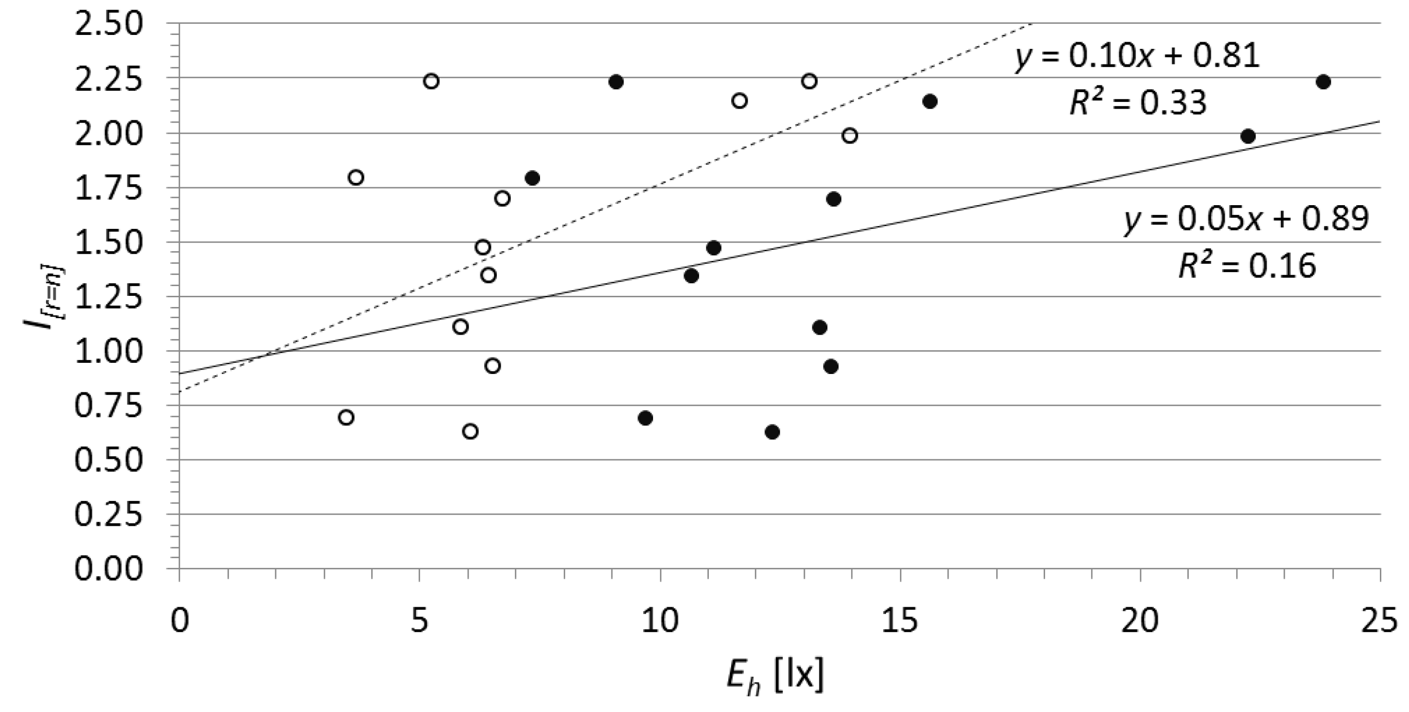
4.1. Correlations in the Case of Scenario 1 (Present Status)
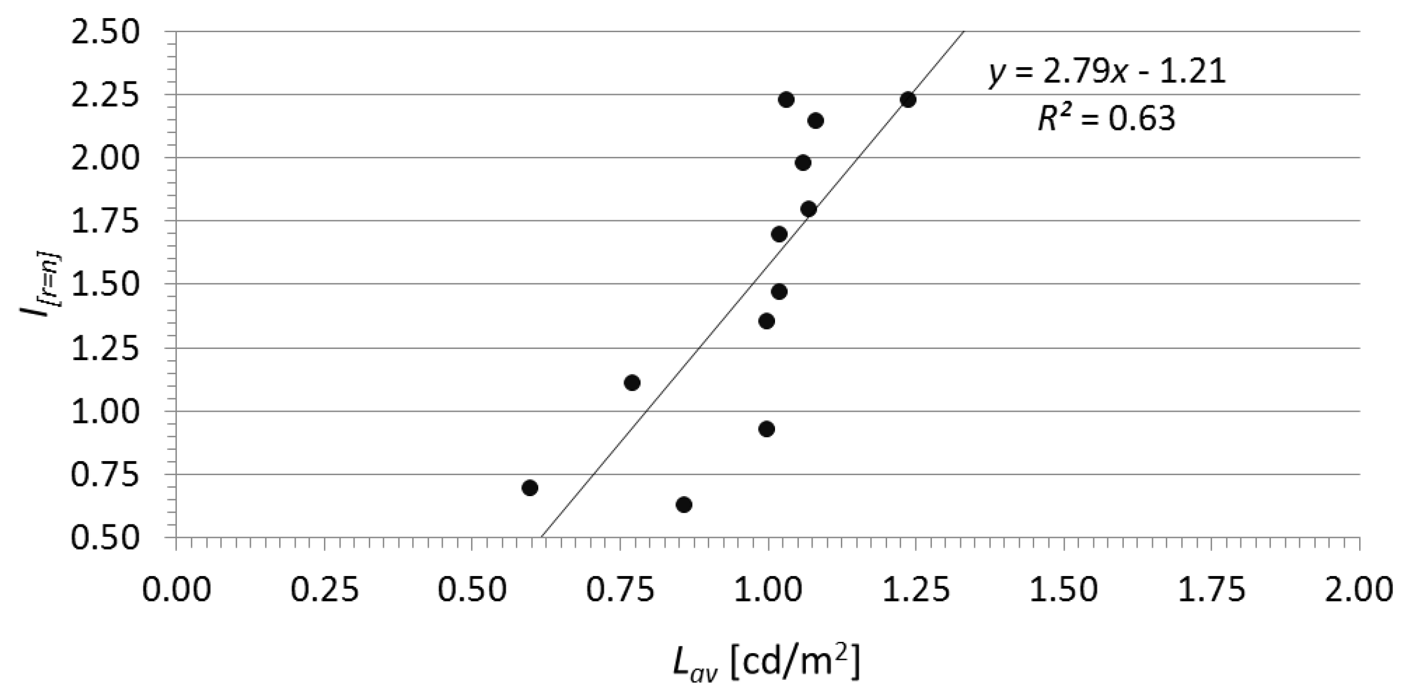
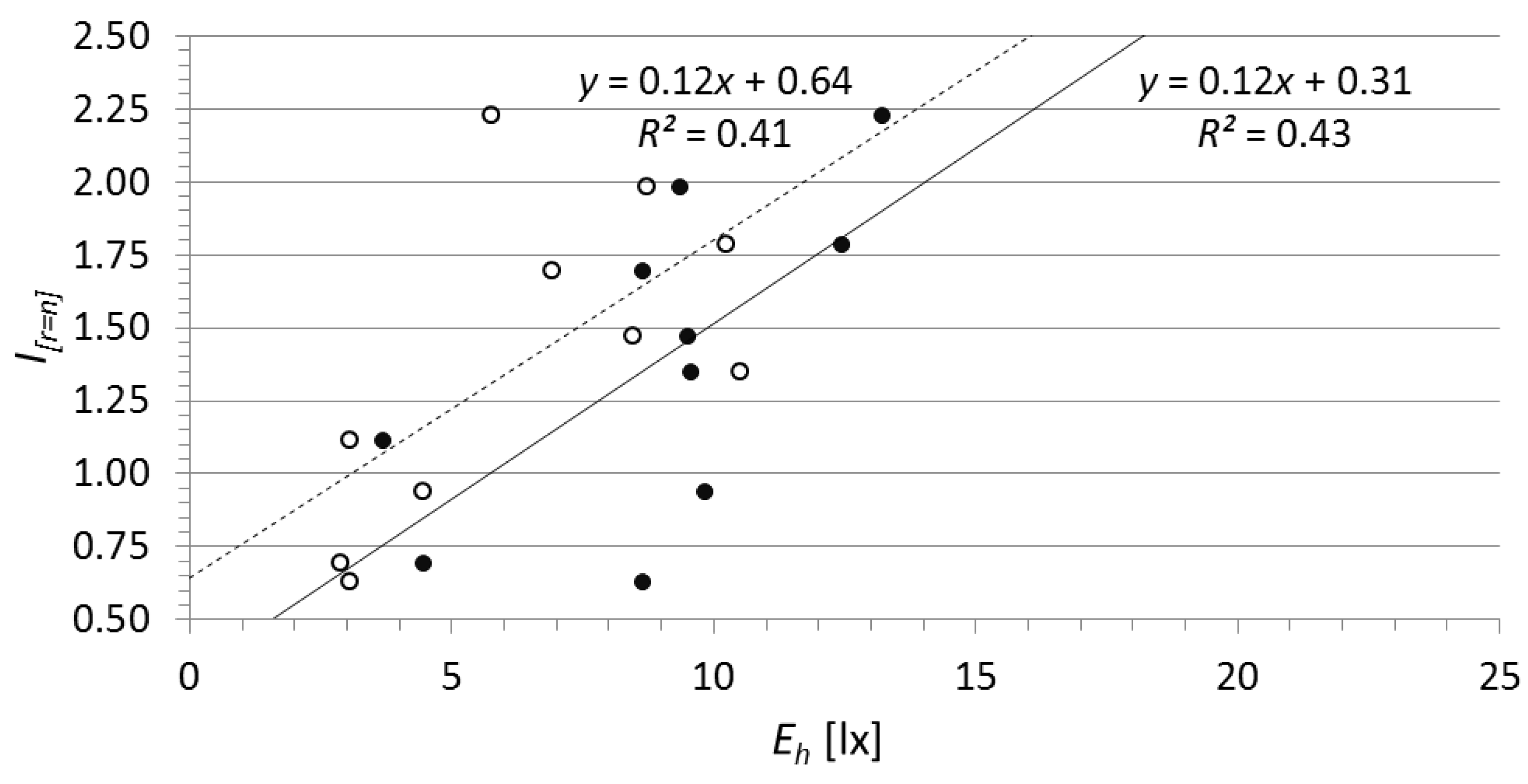
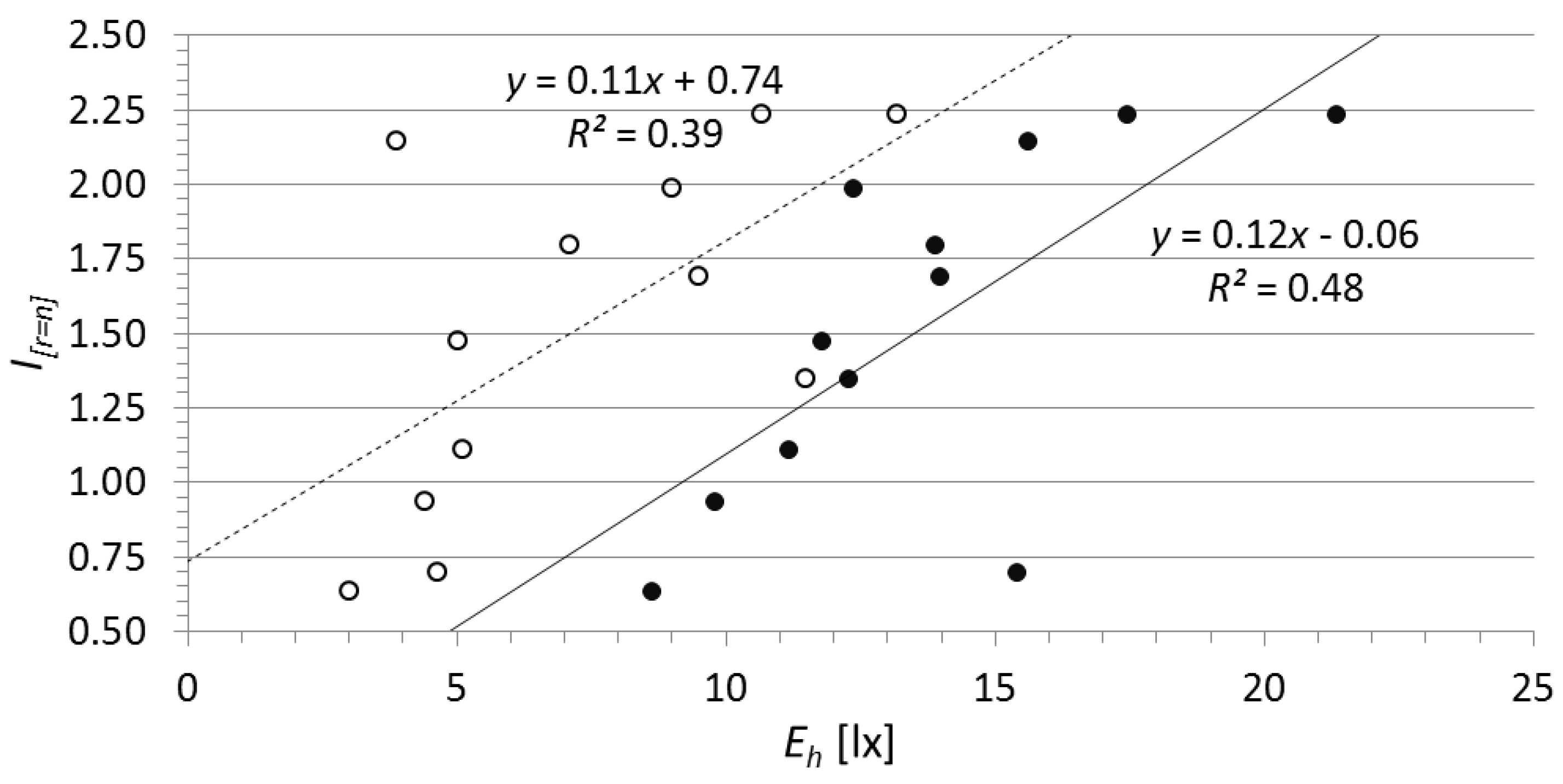
4.2. Correlations in the Case of Scenario 2 (Design Status)
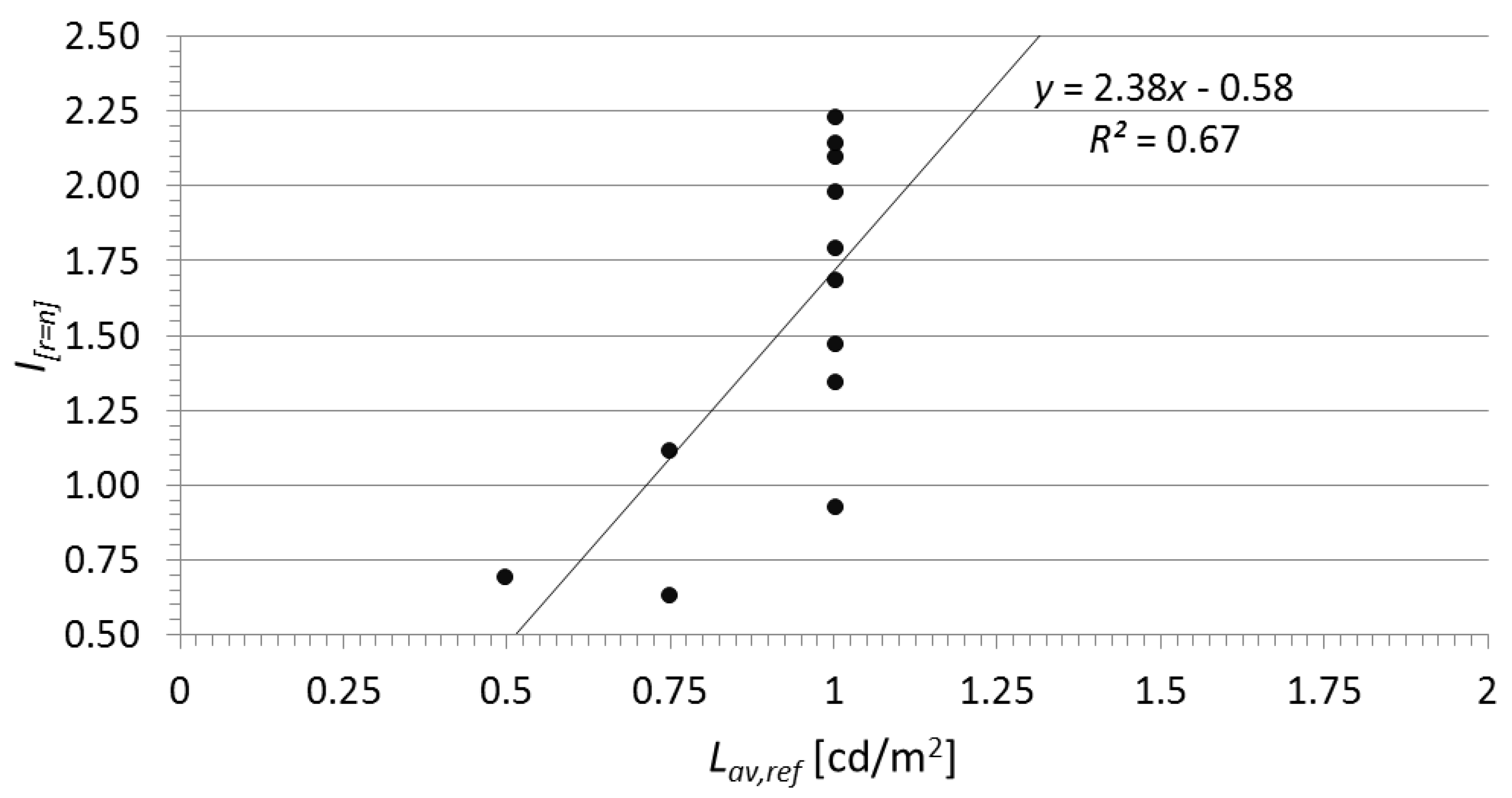
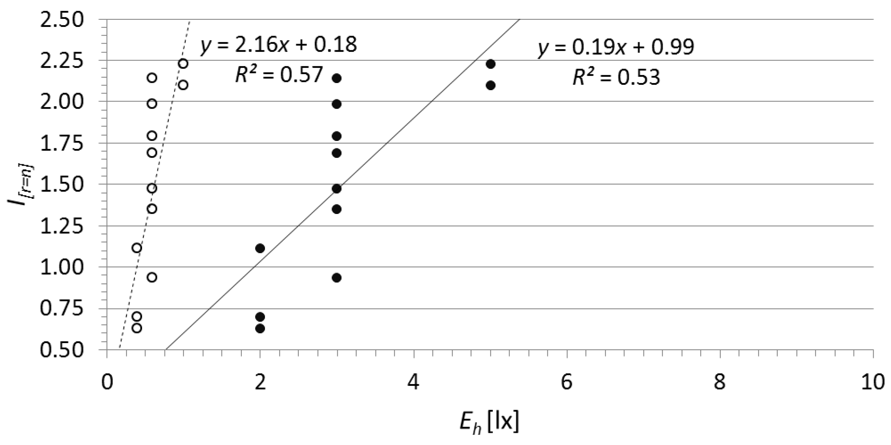
4.3. Correlations in the Case of Scenario 3 (Ideal Case)
5. Discussion and Conclusions
Author Contributions
Funding
Conflicts of Interest
Appendix A

| IPEA Class | IPEA Value | IPEI Class | IPEI Value |
|---|---|---|---|
| A++ | 1.15 < IPEA | A++ | IPEI < 0.75 |
| A+ | 1.10 < IPEA ≤ 1.15 | A+ | 0.75 ≤ IPEI ≤ 0.82 |
| A | 1.05 < IPEA ≤ 1.10 | A | 0.82 ≤ IPEI ≤ 0.91 |
| B | 1.00 < IPEA ≤ 1.05 | B | 0.91 ≤ IPEI ≤ 1.09 |
| C | 0.93 < IPEA ≤ 1.00 | C | 1.09 ≤ IPEI ≤ 1.35 |
| D | 0.84 < IPEA ≤ 0.93 | D | 1.35 ≤ IPEI ≤ 1.79 |
| E | 0.75 < IPEA ≤ 0.84 | E | 1.79 ≤ IPEI ≤ 2.63 |
| F | 0.65 < IPEA ≤ 0.75 | F | 2.63 ≤ IPEI ≤ 3.10 |
| G | IPEA ≤ 0.65 | G | 3.10 ≤ IPEI |
References
- Schivelbusch, W. Disenchanted Night: The Industrialisation of Light in the Nineteenth Century; Berg Publishers: Oxford, UK, 1988. [Google Scholar]
- Seshadri, K. City beautification at night. J. Illum. Eng. Inst. Jpn. 1997, 81, 139–140. [Google Scholar] [CrossRef]
- Leccese, F. Esigenze di comfort della visione notturna e aspetti normative. LUCE 2004, 1, 68–77. [Google Scholar]
- Peña-García, A.; Hurtado, A.; Aguilar-Luzón, M.C. Impact of public lighting on pedestrians’ perception of safety and well-being. Saf. Sci. 2015, 78, 142–148. [Google Scholar] [CrossRef]
- Beccali, M.; Bonomolo, M.; Galatioto, A.; Pulvirenti, E. Smart lighting in a historic context: A case study. Manag. Environ. Qual. 2017, 28, 282–298. [Google Scholar] [CrossRef]
- Bullough, J.D.; Donnell, E.T.; Rea, M.S. To illuminate or not to illuminate: Roadway lighting as it affects traffic safety at intersections. Accid. Anal. Prev. 2013, 53, 65–77. [Google Scholar] [CrossRef] [PubMed]
- Jackett, M.; Frith, W. Quantifying the impact of road lighting on road safety—A New Zealand study. IATSS Res. 2013, 36, 139–145. [Google Scholar] [CrossRef]
- Haans, A.; de Kort, Y.A.W. Light distribution in dynamic street lighting: Two experimental studies on its effects on perceived safety, prospect, concealment and escape. J. Environ. Psychol. 2012, 32, 342–352. [Google Scholar] [CrossRef]
- Elejoste, P.; Angulo, I.; Perallos, A.; Chertudi, A.; García Zuazola, I.J.; Moreno, A.; Azpilicueta, L.; Astrain, J.J.; Falcone, F.; Villadangos, J. An Easy to Deploy Street Light Control System Based on Wireless Communication and LED Technology. Sensors 2013, 13, 6492–6523. [Google Scholar] [CrossRef] [PubMed]
- Karlicek, R.; Sun, C.C.; Zissis, G.; Ma, R. Handbook of Advanced Lighting Technology; Springer: Cham, Switzerland, 2017. [Google Scholar]
- Leccese, F.; Salvadori, G.; Rocca, M. Critical Analysis of the Energy Performance Indicators for Road Lighting Systems in Historical Towns of Central Italy. Energy 2017, 138, 616–628. [Google Scholar] [CrossRef]
- Cutini, V. The Revenge of the Urban Space—The Configurational Approach to the Study and the Analysis of City Centre; Pisa University Press: Pisa, Italy, 2010. [Google Scholar]
- Çamur, K.C.; Roshani, M.; Pirouzi, S. Using space syntax to assess safety in public areas—Case study of Tarbiat pedestrian area, Tabriz-Iran. Mater. Sci. Eng. 2017, 245, 1–9. [Google Scholar] [CrossRef]
- Raval, N.G.; Gundaliya, P.J.; Rajpara, G. Development of model for estimating capacity of roads for heterogenerous traffic condition in urban area. Int. J. Adv. Res. Eng. Sci. Technol. 2017, 4, 198–206. [Google Scholar]
- Kazemidemneh, M.; Mahdavinejad, M. Use of space syntax technique to improve the quality of lighting and modify energy consumption patterns in urban spaces. Eur. J. Sustain. Dev. 2018, 7, 29–40. [Google Scholar] [CrossRef]
- Choi, A.S.; Kim, Y.O.; Oh, E.S.; Kim, Y.S. Application of the space syntax theory to quantitative street lighting design. Build. Environ. 2006, 41, 355–366. [Google Scholar] [CrossRef]
- Turner, A.; Penn, A.; Hillier, B. An algorithmic definition of the axial map. Environ. Plan. B Plan. Des. 2005, 32, 425–444. [Google Scholar] [CrossRef]
- Hillier, B.; Hanson, J. The Social Logic of Space; Cambridge University Press: Cambridge, UK, 1988. [Google Scholar]
- Srisuwan, A. Street lighting design for a traditional city: A case study of Jesi, Italy. WIT Trans. Built Environ. 2011, 121, 13–24. [Google Scholar] [CrossRef]
- Dursun, P. Space syntax in architectural design. In Proceedings of the 6th International Space Syntax Symposium, Istanbul, Turkey, 12–15 June 2007; pp. 1–12. [Google Scholar]
- Xiao, Y. Urban Morphology and Housing Market; Tongji University Press: Shanghai, China, 2017. [Google Scholar]
- Hillier, B.; Penn, A.; Hanson, J.; Grajewski, T.; Xu, J. Natural movement: Or, configuration and attraction in urban pedestrian movement. Environ. Plan. B Plan. Des. 1993, 20, 29–66. [Google Scholar] [CrossRef]
- Azari, A.; Khakzand, M. Context-oriented lighting strategy in urban spaces (using space syntax method) case study: Historical fabric of Isfahan. Int. J. Archit. Eng. Urban Plan. 2014, 24, 37–44. [Google Scholar]
- Cutini, V. Centrality and land use: Three case studies on the configurational hypothesis. Cybergeo Eur. J. Geogr. 2001, 188, 1–10. [Google Scholar] [CrossRef]
- Sharmin, S.; Kamruzzaman, M. Meta-analysis of the relationship between space syntax measures and pedestrian movement. Transp. Rev. 2017, 1–27. [Google Scholar] [CrossRef]
- Cutini, V. Urban space and pedestrian movement: A study on the configurational hypothesis. Cybergeo Eur. J. Geogr. 1999, 111, 1–10. [Google Scholar] [CrossRef]
- Bebhabani, P.A.; Gu, N.; Ostwald, M.J. Comparing the properties of different space syntax techniques for analysing interiors. In Proceedings of the 48th International Conference of the Architectural Science Association, Genova, Italy, 10–13 December 2014; pp. 683–694. [Google Scholar]
- Omer, I.; Kaplan, N.; Jiang, B. Why angular centralities are more suitable for space syntax modelling? In Proceedings of the 11th International Space Syntax Symposium, Lisbon, Portugal, 3–7 July 2017; pp. 1–10. [Google Scholar]
- Turner, A. From isovists to visibility graphs: A methodology for the analysis of architectural space. Environ. Plan. B Plan. Des. 2001, 25, 103–121. [Google Scholar] [CrossRef]
- Kolovou, I.; Gil, J.; Karimi, K.; Law, S.; Versluis, L. Road centre line simplification principles for angular segment analysis. In Proceedings of the 11th International Space Syntax Symposium, Lisbon, Portugal, 3–7 July 2017; pp. 1–16. [Google Scholar]
- Turner, A. Angular Analysis: A Method for the Quantification of Space; UCL: London, UK, 2000. [Google Scholar]
- Dwimirnani, P.; Karimi, K.; Palaiologou, G. Space after dark: Measuring the impact of public lighting at night on visibility, movement and spatial configuration in urban parks. In Proceedings of the 11th Conference on Space Syntax Symposium, Lisbon, Portugal, 3–7 July 2017; pp. 1–18. [Google Scholar]
- Turner, A. Analysing the visual dynamics of spatial morphology. Environ. Plan. B Plan. Des. 2003, 30, 657–676. [Google Scholar] [CrossRef]
- Van der Hoeven, F.; Van Nes, A. Improving the design of urban underground space in metro stations using the space syntax methodology. Tunn. Undergr. Space Technol. 2014, 40, 64–74. [Google Scholar] [CrossRef]
- Van Nes, A.; Yamu, C. Space syntax: Method to measure urban space related to social, economic and cognitive factors. In The Virtual and the Real in Planning and Urban Design: Perspectives, Practices and Applications; Routledge: Oxon, UK, 2018; pp. 136–150. [Google Scholar]
- Turner, A. From axial to road-centre lines: A new representation for space syntax and a new model of route choice for transport network analysis. Environ. Plan. B Plan. Des. 2007, 34, 539–555. [Google Scholar] [CrossRef]
- Di Pinto, V.; Rinaldi, A.M. A configurational approach based on geographic information systems to support decision-making process in real estate domain. Soft Comput. 2018, 1–11. [Google Scholar] [CrossRef]
- D’Autilia, R.; Spada, M. Extension of space syntax methods to generic urban variables. Urban Sci. 2018, 2, 82. [Google Scholar] [CrossRef]
- Paul, A. Unit-segment analysis: A space syntax approach to capturing vehicular travel behaviour emulating configurational properties of roadway structures. Eur. J. Transp. Infrastruct. Res. 2012, 12, 275–290. [Google Scholar]
- Paul, A. A comparative assessment of edge-effect with syntax integration generated in axial and unit-segment approaches to modelling vehicular movement networks. Int. J. Urban Sci. 2014, 18, 340–354. [Google Scholar] [CrossRef]
- Serra, M.; Hiller, B. Spatial configuration and vehicular movement: A nationwide correlational study. In Proceedings of the 11th International Space Syntax Symposium, Lisbon, Portugal, 3–7 July 2017; pp. 1–21. [Google Scholar]
- Cataldo, A.; Di Pinto, V.; Rinaldi, A.M. Representing and sharing spatial knowledge using configurational ontology. Int. J. Bus. Intell. Data Min. 2015, 10, 123–151. [Google Scholar] [CrossRef]
- Ratti, C. The lineage of the line: Space syntax parameters from the analysis of urban DEMs. Environ. Plan. B Plan. Des. 2005, 32, 547–566. [Google Scholar] [CrossRef]
- Omer, I.; Kaplan, N. Using space syntax and agent-based approaches for modelling pedestrian volume at the urban scale. Comput. Environ. Urban Syst. 2017, 64, 57–67. [Google Scholar] [CrossRef]
- Available online: http://www.spacesyntax.net/software/ (accessed on 15 July 2019).
- Turner, A. Depthmap 4—A Researcher’s Handbook; UCL: London, UK, 2004. [Google Scholar]
- Nenci, A.M.; Troffa, R. Integrating space syntax in wayfinding analysis. In Proceedings of the Workshop on Space Syntax and Spatial Cognition, Bremen, Germany, 24 September 2006; pp. 181–184. [Google Scholar]
- International Commission of Illumination. CIE 115—Lighting of Roads for Motor and Pedestrian Traffic, Vienna; International Commission of Illumination: Vienna, Austria, 2010. [Google Scholar]
- European Committee for Standardization. EN 13201-1—Road Lighting—Part 1: Guidelines on Selection of Lighting Classes, Brussels; European Committee for Standardization: Brussels, Belgium, 2015. [Google Scholar]
- European Committee for Standardization. EN 13201-2—Road Lighting—Part 2: Performance Requirements, Brussels; European Committee for Standardization: Brussels, Belgium, 2015. [Google Scholar]
- European Committee for Standardization. EN 13201-3—Road Lighting—Part 3: Calculation of Performance, Brussels; European Committee for Standardization: Brussels, Belgium, 2015. [Google Scholar]
- European Committee for Standardization. EN 13201-4—Road Lighting—Part 4: Methods of Measuring Lighting Performance, Brussels; European Committee for Standardization: Brussels, Belgium, 2015. [Google Scholar]
- European Committee for Standardization. EN 13201-5—Road Lighting—Part 5: Energy Performance Indicators, Brussels; European Committee for Standardization: Brussels, Belgium, 2015. [Google Scholar]
- Ente Nazionale Italiano di Unificazione. UNI 11248—Road Lighting—Selection of Lighting Classes, Milan; Ente Nazionale Italiano di Unificazione: Milan, Italy, 2016. [Google Scholar]
- Regional Council of Emilia Romagna. Standards on Reduction of Light Pollution and Energy Savings; Regional Council of Emilia Romagna: Bologna, Italy, 2015. [Google Scholar]
- International Organization for Standardization. ISO/CIE 19476—Characterization of the Performance of Illuminance Meters and Luminance Meters, Geneva; International Organization for Standardization: Geneva, Switzerland, 2014. [Google Scholar]
- Available online: https://www.dial.de/en/dialux/ (accessed on July 2019).
- International Commission of Illumination. CIE 154—The Maintenance of Outdoor Lighting Systems, Vienna; International Commission of Illumination: Vienna, Austria, 2003. [Google Scholar]
- Beccali, M.; Bonomolo, M.; Leccese, F.; Lista, D.; Salvadori, G. On the impact of safety requirements, energy prices and investment costs in street lighting refurbishment design. Energy 2018, 165, 739–759. [Google Scholar] [CrossRef]
- Beccali, M.; Bonomolo, M.; Lo Brano, V.; Ciulla, G.; Di Dio, V.; Massaro, F.; Favuzza, S. Energy saving and user satisfaction for a new advanced public lighting system. Energy Convers. Manag. 2019, 195, 943–957. [Google Scholar] [CrossRef]


| Group | I | Number of Roads | Number of Selected Roads |
|---|---|---|---|
| A | 2.48 ≤ I ≤ 2.16 | 37 (12.2%) | 5 (12.2%) |
| B | 2.16 < I ≤ 1.84 | 38 (12.5%) | 5 (12.5%) |
| C | 1.84 < I ≤ 1.52 | 69 (22.5%) | 9 (22.5%) |
| D | 1.52 < I ≤ 1.20 | 46 (15.0%) | 6 (15.0%) |
| E | 1.20 < I ≤ 0.88 | 76 (25.0%) | 10 (25.0%) |
| F | 0.88 < I ≤ 0.56 | 39 (12.8%) | 5 (12.8%) |
| Tot. | 305 (100.0%) | 40 (100.0%) |
| Road ID | Traffic Volumes | Road ID | Traffic Volumes | ||
|---|---|---|---|---|---|
| Pedestrian | Motorised | Pedestrian | Motorised | ||
| 1 | 85 | 80 | 21 | 18 | 34 |
| 2 | 183 | 178 | 22 | 45 | 51 |
| 3 | 60 | 64 | 23 | 7 | 5 |
| 4 | 69 | 61 | 24 | 17 | 18 |
| 5 | 104 | 98 | 25 | 23 | 25 |
| 6 | 21 | 15 | 26 | 24 | 37 |
| 7 | 36 | 43 | 27 | 12 | 9 |
| 8 | 91 | 64 | 28 | 12 | 11 |
| 9 | 23 | 19 | 29 | 12 | 14 |
| 10 | 38 | 43 | 30 | 13 | 9 |
| 11 | 29 | 32 | 31 | 20 | 22 |
| 12 | 33 | 29 | 32 | 16 | 18 |
| 13 | 20 | 5 | 33 | 21 | 28 |
| 14 | 28 | 41 | 34 | 15 | 21 |
| 15 | 49 | 65 | 35 | 10 | 14 |
| 16 | 14 | 8 | 36 | 4 | 3 |
| 17 | 80 | 70 | 37 | 17 | 26 |
| 18 | 23 | 18 | 38 | 3 | 2 |
| 19 | 6 | 5 | 39 | 4 | 1 |
| 20 | 17 | 25 | 40 | 8 | 5 |
| Space Syntax Techniques | Spatial Indicators | R2 | |
|---|---|---|---|
| Pedestrian Traffic Volumes | Motorised Traffic Volumes | ||
| Axial analysis | Integration index, I | 0.69 | 0.59 |
| Choice index, Ch | 0.33 | 0.29 | |
| Angular segment analysis | Integration index, I | 0.64 | 0.54 |
| Choice index, Ch | 0.35 | 0.37 | |
| Road ID | Lighting Class | Minimum Lighting Requirements | |||
|---|---|---|---|---|---|
| Carriageway | Sidewalk | Carriageway | Sidewalk | ||
| Lav,ref [cd/m2] | Eh,av,ref [lx] | Eh,min,ref [lx] | |||
| 1 | M3 | P3 | 1.0 | 5.0 | 1.0 |
| 2 | M3 | P3 | 1.0 | 5.0 | 1.0 |
| 3 | M3 | P5 | 1.0 | 3.0 | 0.6 |
| 4 | M3 | P5 | 1.0 | 3.0 | 0.6 |
| 5 | M3 | P5 | 1.0 | 3.0 | 0.6 |
| 6 | M3 | P5 | 1.0 | 3.0 | 0.6 |
| 7 | M3 | P5 | 1.0 | 3.0 | 0.6 |
| 8 | M3 | P5 | 1.0 | 3.0 | 0.6 |
| 9 | M4 | P6 | 0.8 | 2.0 | 0.4 |
| 10 | M3 | P5 | 1.0 | 3.0 | 0.6 |
| 11 | M5 | P6 | 0.5 | 2.0 | 0.4 |
| 12 | M4 | P6 | 0.8 | 2.0 | 0.4 |
| ID | r [m] | lc [m] | lss [m] | Lso [m] | i | p1 [m] | p2 [m] | LID | d [m] | h [m] | t [°] | n | |
|---|---|---|---|---|---|---|---|---|---|---|---|---|---|
| 1 | 466 | 7.00 | 3.45 | – | one sided | 3.95 | – | A | 33.50 | 10.50 | 15 | 13 | |
| 2 | 431 | 5.50 | 3.10 | 1.80 | two sided staggered | 3.40 | 3.60 | B | 24.00 | 8.00 | 5 | 31 | |
| 3 | 735 | 10.00 | 3.00 | – | one-sided | 6.15 | – | C | 25.00 | 8.00 | 0 | 30 | |
| 4 | 109 | 5.60 | 1.00 | 0.60 | one-sided | 2.80 | – | D | 18.00 | 7.50 | 15 | 6 | |
| 5 | 350 | 8.00 | 1.45 | 1.45 | one-sided | 4.45 | – | A | 41.00 | 12.00 | 5 | 7 | |
| 6 | 408 | 12.20 | 1.50 | 2.50 | one-sided | 6.25 | – | E | 20.50 | 8.00 | 15 | 21 | |
| 7 | 295 | 8.30 | 1.45 | 1.45 | one-sided | 4.45 | – | A | 24.10 | 8.00 | 5 | 10 | |
| 8 | 337 | 7.00 | 1.20 | 1.00 | one-sided | 3.55 | – | F | 22.50 | 9.00 | 15 | 13 | |
| 9 | 204 | 7.00 | 0.90 | 0.90 | one-sided | 4.20 | – | G | 22.00 | 6.00 | 15 | 8 | |
| 10 | 442 | 7.00 | 2.40 | 2.40 | two sided staggered | 4.70 | 5.70 | H | 50.00 | 7.00 | 5 | 18 | |
| 11 | 241 | 3.50 | 1.00 | 1.00 | one-sided | 2.45 | – | I | 12.00 | 3.50 | 0 | 19 | |
| 12 | 111 | 6.75 | 1.60 | 1.60 | two sided staggered | 3.78 | 3.78 | G | 40.00 | 6.00 | 0 | 5 | |
 | |||||||||||||
| LID | P [W] | Φ [lm] | η [lm/W] | S | Tc [K] | Photometry | Image |
|---|---|---|---|---|---|---|---|
| A | 166 | 13,194 | 79 | HPS | 2000 |  |  |
| B | 158 | 10,897 | 69 | MH | 3000 | 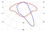 |  |
| C | 118 | 6099 | 52 | LED | 4200 | 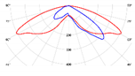 |  |
| D | 114 | 7546 | 66 | HPS | 2000 | 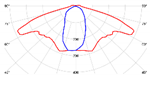 | 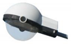 |
| E | 169 | 11,412 | 68 | MH | 3000 | 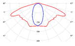 | 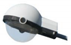 |
| F | 114 | 6700 | 59 | MH | 4200 |  | 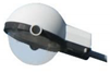 |
| G | 157 | 9988 | 64 | MH | 3000 | 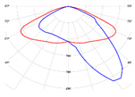 | 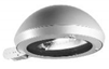 |
| H | 118 | 6099 | 52 | MH | 4200 | 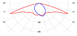 |  |
| I | 116 | 2430 | 21 | HPS | 2100 |  |  |
| Road ID | Carriageway | Sidewalk (on Luminaire Side) | Sidewalk (on the Opposite Luminaire Side) | ||
|---|---|---|---|---|---|
| Lav [cd/m2] | Eh,av [lx] | Eh,min [lx] | Eh,av [lx] | Eh,min [lx] | |
| 1 | 0.7 | 21.4 | 11.9 | – | – |
| 2 | 0.9 | 8.6 | 4.9 | 6.6 | 3.8 |
| 3 | 0.9 | 13.9 | 11.5 | – | − |
| 4 | 1.9 | 21.3 | 12.3 | 10.6 | 8.3 |
| 5 | 0.6 | 6.7 | 3.5 | 7.4 | 5.2 |
| 6 | 1.1 | 12.1 | 6.0 | 3.7 | 2.6 |
| 7 | 0.8 | 10.0 | 5.8 | 6.3 | 5.8 |
| 8 | 0.5 | 10.4 | 6.4 | 4.7 | 3.5 |
| 9 | 0.8 | 12.4 | 5.6 | 13.0 | 10.9 |
| 10 | 1.2 | 13.3 | 6.4 | 12.8 | 5.6 |
| 11 | 0.6 | 9.1 | 3.3 | 5.0 | 3.3 |
| 12 | 1.2 | 11.0 | 5.5 | 10.8 | 5.9 |
| Road ID | Carriageway | Sidewalk (on Luminaire Side) | Sidewalk (on the Opposite Luminaire Side) | |||||||
|---|---|---|---|---|---|---|---|---|---|---|
| Lav [cd/m2] | (%) | Eh,av [lx] | (%) | Eh,min [lx] | (%) | Eh,av [lx] | (%) | Eh,min [lx] | (%) | |
| 1 | 0.72 | 3 | 23.8 | 11 | 13.1 | 10 | – | – | – | – |
| 2 | 0.98 | 9 | 9.09 | 6 | 5.24 | 7 | 7.44 | 13 | 3.97 | 4 |
| 3 | 0.96 | 7 | 15.6 | 12 | 11.7 | 2 | – | – | – | – |
| 4 | 1.98 | 4 | 22.2 | 4 | 14.0 | 14 | 11.5 | 8 | 9.12 | 10 |
| 5 | 0.67 | 12 | 7.33 | 9 | 3.68 | 5 | 8.00 | 8 | 5.80 | 12 |
| 6 | 1.27 | 15 | 13.7 | 13 | 6.74 | 12 | 4.08 | 10 | 2.63 | 1 |
| 7 | 0.86 | 7 | 11.2 | 12 | 6.32 | 9 | 6.88 | 9 | 6.06 | 4 |
| 8 | 0.57 | 14 | 10.7 | 3 | 6.46 | 1 | 4.90 | 4 | 3.80 | 9 |
| 9 | 0.91 | 14 | 13.3 | 7 | 5.88 | 5 | 14.8 | 14 | 12.3 | 13 |
| 10 | 1.38 | 15 | 13.6 | 2 | 6.56 | 2 | 13.6 | 6 | 6.11 | 9 |
| 11 | 0.60 | 0 | 9.72 | 7 | 3.46 | 5 | 5.20 | 4 | 3.51 | 6 |
| 12 | 1.36 | 13 | 12.3 | 12 | 6.06 | 10 | 12.3 | 14 | 6.06 | 3 |
| LID | P [W] | Φ [lm] | η [lm/W] | S | Tc [K] | Photometry | Image | Road of Installation (ID Number) |
|---|---|---|---|---|---|---|---|---|
| L | 138 | 14,663 | 106 | LED | 4000 | 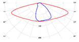 |  | 1, 5 |
| M | 63 | 7083 | 112 | LED | 4000 | 3, 7, 8, 12 | ||
| N | 56 | 5742 | 103 | LED | 4000 | 2, 6, 10 | ||
| O | 32 | 3305 | 103 | LED | 4000 | 4, 9, 11 |
| Road ID | Carriageway | Sidewalk (on Luminaire Side) | Sidewalk (on the Opposite Luminaire Side) | ||
|---|---|---|---|---|---|
| Lav [cd/m2] | Eh,av [lx] | Eh,min [lx] | Eh,av [lx] | Eh,min [lx] | |
| 1 | 1.03 | 21.4 | 13.2 | – | – |
| 2 | 1.24 | 17.5 | 10.7 | 13.2 | 5.75 |
| 3 | 1.08 | 15.7 | 3.93 | – | – |
| 4 | 1.06 | 12.4 | 9.02 | 9.34 | 8.76 |
| 5 | 1.07 | 13.9 | 7.11 | 12.4 | 10.2 |
| 6 | 1.02 | 14.0 | 9.49 | 8.66 | 6.93 |
| 7 | 1.02 | 11.8 | 5.07 | 9.51 | 8.50 |
| 8 | 1.00 | 12.3 | 11.5 | 9.56 | 10.5 |
| 9 | 0.77 | 11.2 | 5.16 | 3.69 | 3.05 |
| 10 | 1.00 | 9.82 | 4.45 | 9.82 | 4.45 |
| 11 | 0.60 | 15.4 | 4.66 | 4.49 | 2.90 |
| 12 | 0.86 | 8.62 | 3.05 | 8.62 | 3.05 |
| Scenario | Carriageway | Sidewalk (on Luminaire Side) | Sidewalk (on the Opposite Luminaire Side) | ||
|---|---|---|---|---|---|
| Lav [cd/m2] | Eh,av [lx] | Eh,min [lx] | Eh,av [lx] | Eh,min [lx] | |
| 1 (present status) | 7.6 × 10⁻⁴ | 0.16 | 0.33 | 0.08 | 4.7 × 10⁻³ |
| 2 (design status) | 0.63 (63%) | 0.48 (32%) | 0.39 (6%) | 0.43 (35%) | 0.41 (41%) |
| 3 (ideal case) | 0.67 (67%) | 0.53 (37%) | 0.53 (20%) | 0.53 (45%) | 0.53 (53%) |
© 2019 by the authors. Licensee MDPI, Basel, Switzerland. This article is an open access article distributed under the terms and conditions of the Creative Commons Attribution (CC BY) license (http://creativecommons.org/licenses/by/4.0/).
Share and Cite
Leccese, F.; Lista, D.; Salvadori, G.; Beccali, M.; Bonomolo, M. Space Syntax Analysis Applied to Urban Street Lighting: Relations between Spatial Properties and Lighting Levels. Appl. Sci. 2019, 9, 3331. https://doi.org/10.3390/app9163331
Leccese F, Lista D, Salvadori G, Beccali M, Bonomolo M. Space Syntax Analysis Applied to Urban Street Lighting: Relations between Spatial Properties and Lighting Levels. Applied Sciences. 2019; 9(16):3331. https://doi.org/10.3390/app9163331
Chicago/Turabian StyleLeccese, Francesco, Davide Lista, Giacomo Salvadori, Marco Beccali, and Marina Bonomolo. 2019. "Space Syntax Analysis Applied to Urban Street Lighting: Relations between Spatial Properties and Lighting Levels" Applied Sciences 9, no. 16: 3331. https://doi.org/10.3390/app9163331
APA StyleLeccese, F., Lista, D., Salvadori, G., Beccali, M., & Bonomolo, M. (2019). Space Syntax Analysis Applied to Urban Street Lighting: Relations between Spatial Properties and Lighting Levels. Applied Sciences, 9(16), 3331. https://doi.org/10.3390/app9163331