Article

Sensorless Air Flow Control in an HVAC System through Deep Learning

1
A&B Center, CTO, LG Electronics, Seoul 08592, Korea
2
Department of Computer Science and Engineering, Korea University, Seoul 02841, Korea
*
Author to whom correspondence should be addressed.
Gasan R&D Campus, LG Electronics, 51, Gasan digital 1-ro, Geumcheon-gu, Seoul 08592, Korea.
Department of Computer Science and Engineering, Korea University, Anam-Dong, Sungbuk-Gu, Seoul 02841, Korea.
Appl. Sci. 2019, 9(16), 3293; https://doi.org/10.3390/app9163293
Submission received: 16 June 2019 / Revised: 31 July 2019 / Accepted: 9 August 2019 / Published: 11 August 2019
(This article belongs to the Special Issue Intelligence Systems and Sensors)

Abstract

:
Sensor-based intelligence is essential in future smart buildings, but the benefits of increasing the number of sensors come at a cost. First, purchasing the sensors themselves can incur non-negligible costs. Second, since the sensors need to be physically connected and integrated into the heating, ventilation, and air conditioning (HVAC) system, the complexity and the operating cost of the system are increased. Third, sensors require maintenance at additional costs. Therefore, we need to pursue the appropriate technology (AT) in terms of the number of sensors used. In the ideal scenario, we can remove excessive sensors and yet achieve the intelligence that is required to operate the HVAC system. In this paper, we propose a method to replace the static pressure sensor that is essential for the operation of the HVAC system through the deep neural network (DNN).

1. Introduction

Of the global energy consumption, the energy used by buildings worldwide is over 40%, among which heating, ventilation, and air conditioning (HVAC) systems account for nearly 40–70% [1]. For this reason, much research has been carried out to improve the operating efficiency of the HVAC system. One essential component of these efforts is the sensor. For instance, researchers have found that energy savings can be obtained by interlocking the sensor in the building with the control device [2,3,4]. Furthermore, HVAC system faults can be diagnosed by analyzing the sensor data so that the energy waste and failure of the device can be prevented [5]. In recent years, studies have been actively attempting to integrate artificial intelligence technology with such systems to improve the intelligence and utilization of sensors. In particular, research is underway to reduce energy by forecasting the energy demand and supply [6], designing automatic fault detection technology using deep learning methods [5,7], and developing smart sensors with artificial intelligence (AI) [8]. Because the data used to train the AI come from the sensors, they are essential for enhancing the intelligence of buildings. Therefore, an increasing number of sensors are expected to be used in future smart buildings.
However, the pursuit of sensor-based intelligence should account for the fact that the benefits of using an increasing number of sensors come at a cost. First, purchasing the sensors themselves can incur non-negligible costs. For instance, each static pressure sensor used in the HVAC system costs $500–600, and at least one static pressure sensor is required for each Air Handling Unit (AHU). Second, the sensors need to be physically connected and integrated into the HVAC system. This increases the complexity and operating cost of the system. Third, sensors require maintenance at additional costs. The sensors can be subject to faults or miscalibration, in which case they need to be repaired or replaced. In some cases, the sensors are located in places that maintenance personnel cannot easily reach. It is not uncommon for an HVAC system to have many components situated near the ceiling or in ducts. Therefore, the holy grail of the sensor-based intelligent HVAC system should be the appropriate technology (AT) in terms of the number of sensors used. In the ideal scenario, we can use the minimum number of sensors required to achieve the intelligence that we need to operate the HVAC system.
The target system in this paper is the Air Handling Unit (AHU) in the HVAC system. The AHU regulates and circulates the air, and its components include a blower, heating or cooling elements, filter racks or chambers, sound attenuators, and dampers [9]. It connects to a ductwork system that distributes the conditioned air throughout the building, after which the air returns to the AHU. The AHU needs fan control to blow conditioned air at an appropriate pressure. For this purpose, the AHU system needs to determine the static pressure in the path of the air flow. For this purpose, a static pressure sensor is installed in the ceiling duct that forms the air flow path, as shown in Figure 1. The air flow between the AHU and the room is depicted in Figure 2. The sensor reports the measured pressure inside the duct to the AHU so that the AHU can regulate the air flow using fan control if necessary. Because of its location in the system, however, the integration and the maintenance of the sensor can be burdensome and costly, in addition to the cost of the sensor itself. Therefore, in this paper, we investigate the possibility of removing the static pressure sensor from the target Air Handling Unit (AHU) system while achieving the level of predicted pressure values that are comparable to the measured values.
In this paper, we propose a method to predict the operating dynamics of s HVAC system without a static pressure sensor through a deep learning approach. Through this method, we can operate the HVAC system without a static pressure sensor utilizing other available sensors such as temperature, fan speed, and airflow sensors, hence reducing costs for HVAC system operation. In addition, we have also demonstrated an innovative technique to replace the physical sensor value with the logical Deep Neural Network (DNN) method through the proposed method.
In terms of the immediate value and the future applicability of the model, the contributions of this paper are as follows:
  • This paper demonstrates that a Long Short-Term Memory (LSTM)-based predictor can replace a static pressure sensor component using a real AHU. This approach can reduce costs in many ways: the hardware cost ($500–600 per sensor) for each AHU, the installation and operational cost, and the maintenance cost.
  • This paper explores the impacts of various input parameters and processing steps on the performance of the LSTM-based multivariate time-series prediction. It provides insight into optimization that can be applied to similar systems.
  • This paper shows that the developed prediction model can be applied to HVAC systems with different capacities and in different seasonal conditions.
The remainder of this paper is organized as follows: Section 2 summarizes the application of artificial intelligence to HVAC systems and the research on how to replace sensors. Section 3 describes the deep learning model for static pressure prediction. The model configuration and selected input and output elements are explained. Section 4 describes the data used in the experiment and the hyperparameters applied to the proposed model. In this section, the results of the experiment are analyzed and discussed. Finally, the conclusions of this paper are given in Section 5.

2. Related Work

In this section, we briefly survey the previous work on two subjects that are relevant to this paper. The first is the recent trend of applying artificial intelligence (AI) to the operation of HVAC systems, and the second is the development of sensorless HVAC operation methods. First, we examine AI techniques in the context of HVAC system design.
For the control and management of the HVAC system, there have been two main threads of research on the application of AI to HVAC system control. The first is performance optimization of the HVAC system, and the second is fault management. For the former approach, various operating techniques using a DNN have been studied as methods for efficient HVAC system control. Jonathan et al. [6] used an artificial neural network to predict energy use and optimize the energy supply as an optimization method. Kato et al. [10] proposed a thermal load prediction technique that was more efficient than the Multi-Layer Perceptron (MLP) method by applying three hidden layers in a Recurrent Neural Network (RNN) approach. José et al. [11] proposed a method of optimal energy supply for control and demand by minimizing energy use through a Deep Reinforcement Learning (DRL) method using two hidden layers. They introduced model-free and self-learning HVAC system control using their proposed method. Park et al. [12] applied reinforcement learning to a general room detection method to improve its performance. The method allows for the control of illumination through the user’s smartphone and adjusts the illumination according to the light sensor value. Using a genetic algorithm, Sokratis et al. [13] proposed the possibility of a zero-energy building with and without occupancy as a means to optimally control temperature set-points in different climates. William et al. [14] introduced a method that achieved 4–5% energy savings and 10% CO 2 savings through HVAC control using deep reinforcement learning. For HVAC system fault management, artificial intelligence has been leveraged to perform fault diagnosis and fault prediction of the equipment. Conventional methods of modeling a facility and detecting faults operate on the basis of historical fault data. However, Hadi et al. [5] used an RNN model-based fault diagnosis technique with a time step of 1 to detect faults without such data. Rahat et al. [7] used a deep autoencoder [15] and Artificial Neural Network (ANN) to provide various data for fault detection in the industry, and its performance was twice as high as the conventional rule-based method. Lee et al. [16] detected more than 95% of the faults in an Air Handling Unit (AHU) using five hidden layers with 200 neurons. Yabin et al. [17] also detected 97% of the faults in a variable refrigerant flow system using a DNN. This fault detection method enables the facility administrator to check the status and cause of the fault and to return the plant operation to its normal state quickly by effectively troubleshooting the problem. The deep learning method used for the operation and fault detection of the HVAC system uses a time-series RNN structure, rather than simply learning using multiple layers. Because the HVAC system is operated to achieve target control using the current state and creates the state of the future, all related data have time-series characteristics. This approach is also required to predict the static pressure in a duct in the study reported here. A few existing works have followed the sensorless operation research thread, although most of them have not been in the HVAC domain. In the field of motor control, sensorless control has been applied for a long time [18,19,20]. Recently, intelligent motor control using an RNN has been studied [21,22]. Further research is underway to replace the difficult and expensive sensors installed in the field of wind and solar energy, which are new and renewable energy sources, by applying a prediction method using DNN. Shahaboddin et al. [23] predicted wind speed using the rotor speed and other variables of the wind power source using an adaptive neuro-fuzzy inference system. Vlastimir et al. [24] proposed a model with higher airspeed prediction accuracy than that of conventional methods using a feed-forward neural network with multiple hidden neurons and support vector machine. Kumar et al. [25] estimated flow meter values using a four-layer forward neural network and fuzzy training. Their results showed an error rate of 3.28% compared with the actual flow value. Predicting the value of the flow meter from the flow rate in a system that controls the valve has shown that the system is able to operate without a sensor.
In this paper, we propose a deep learning-based approach to predicting HVAC system dynamics without using sensors. Using this method, we demonstrate that the static pressure sensor is not required to achieve efficient HVAC operation, hence reducing costs for installing and operating HVAC systems.

3. Predicting Static Pressure Using Deep Learning

In this section, we introduce a static pressure sensor prediction model for HVAC systems using Deep Neural Networks (DNNs). Since the static pressure and the input data used for the static pressure prediction have time-series characteristics, the Recurrent Neural Network (RNN) model is expected to be the most effective for learning multivariate time-series data. Among the RNN variants, we utilized the LSTM method, which avoids the vanishing gradient issue of the Vanilla RNN. This is discussed in Section 3.1 and Section 3.2 in more detail.
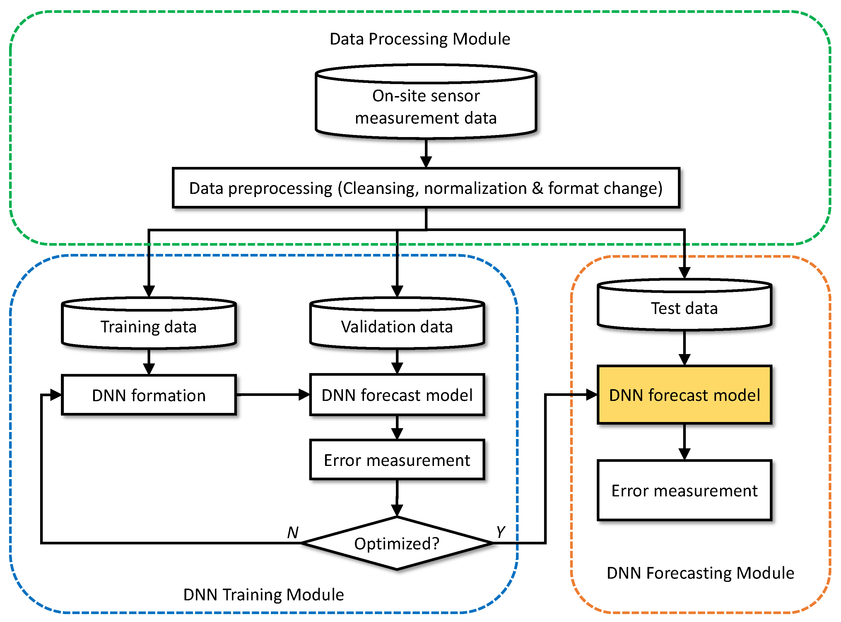
For the LSTM model, we identified various factors that affect the static pressure in the HVAC operation when it is adjusted according to the difference between the set-point static pressure and the current static pressure. Then, we analyzed the data characteristics of these selected input values. We used part of the accumulated data sets, which consist of multiple variables in chronological order, to train and validate the LSTM. Of the data sets used for the purpose, we used 20% for validation and 80% for training. Then, we used the LSTM to predict the current static pressure using input that was not used for training or validation. Figure 3 shows the overall flow of the training, validation, and test processes.
Our proposed prediction model achieved a mean absolute percentage error (MAPE) of 2.45%. Below, we discuss the details of the LSTM model used for our prediction model, as well as the input data used to train it.

3.1. Input Data Characteristics

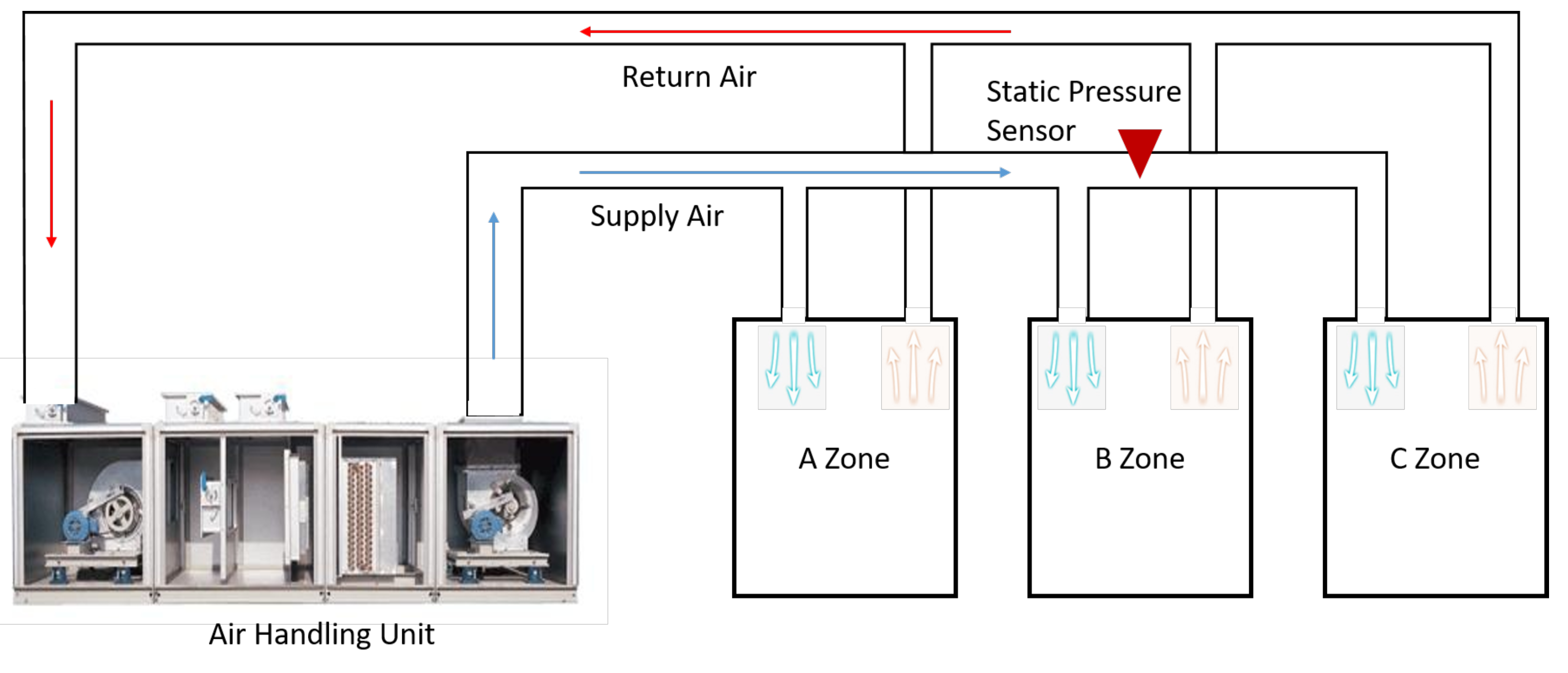
In the HVAC system structure shown in Figure 4, the Air Handling Unit (AHU) has a supply fan and a return fan that blow air into the room and suck air out of it, respectively. Each fan is an inverter type and can adjust its speed. The speed of the supply fan is controlled by the static pressure of the supply duct and the set-point of static pressure, and the return fan operates at a similar speed to that of the supply fan. The amount and temperature of the wind supplied to the room are measured and regulated to maintain a set temperature for the room.
Before developing the LSTM model, we identified the environmental factors that affect the static pressure in the duct and analyzed their characteristics. In particular, we determined whether these factors exhibit temporal variations or specific patterns. For instance, Figure 5 shows the set-point values of the static pressure and the other measured values for the 4th floor data set, one of the three floors for which we accumulated data. In the figure showing data for the 4th floor, the set-point pressure and the measured pressure are related. They are also related to the fan speed and the air flows into and out of the duct. The supply and return air temperature fluctuations are also related to the set-point temperature. When cooling or heating, the fan speed depends on the set-point temperature and the temperature of the returning air. The speed is higher when the temperature difference is larger.
Thus, the direct factors that affect the static pressure in the duct are the set-point for the static pressure, the operating speed of the supply fan, the supply air volume, and the return air volume. The factors that affect the air volume are the set-point of the temperature, the current temperature (supply and return air), and the speed of the supply fan. These values are required inputs to the LSTM. We selected seven input parameters that directly or indirectly affect the system dynamics for the deep learning model. They are
  • Set-point of the static pressure (Millimeter Aqua; mmAq),
  • Set-point of the temperature ( C),
  • Volume of the supply air (Cubic Feet per Minute; CFM),
  • Volume of the return air (CFM),
  • Temperature of the supply air ( C),
  • Temperature of the return air ( C),
  • Speed of the inverter fan (Hz).
Except for the set-points of the temperature and static pressure, all data used are time-series data. To train the LSTM model, we used three historical data sets obtained from our HVAC system. The commonalities of these data sets are as follows:
  • All data sets are for a four-month period, from May through August, and were collected at 1-min intervals from 12:00 a.m. to 11:59 p.m.
  • All data sets consist of operational data from spring (from May to June) and summer (from July to August). These two periods have different operational targets because the HVAC system only blows air in spring, but it supplies cold air in summer.
  • All data sets were subjected to the HVAC system test at varying static pressures from 10 August to the end of August.
On the other hand, the data sets come from different floors in the same building: floors 4, 5, and 6. The HVAC system structure of each floor is the same, but the designed capacity is set differently according to the amount of heat generated. The 4th floor is an office space that generates the least heat, and the 6th floor is a laboratory that generates the most heat. The 5th floor is part laboratory and part office space, so the generated heat is between the heat produced on the 4th and 6th floors. Consequently, the static pressure set-point is determined differently.
The static pressure is zero millimeter Aqua (mmAq) when the system is in the stopped state. Otherwise, the system is in operation. Since the input values have significantly different ranges, it was necessary to normalize them to improve the learning performance before we applied our deep learning model. Normalization was performed by converting each data point to a value between 0 and 1, which represent the maximum and minimum values, respectively.
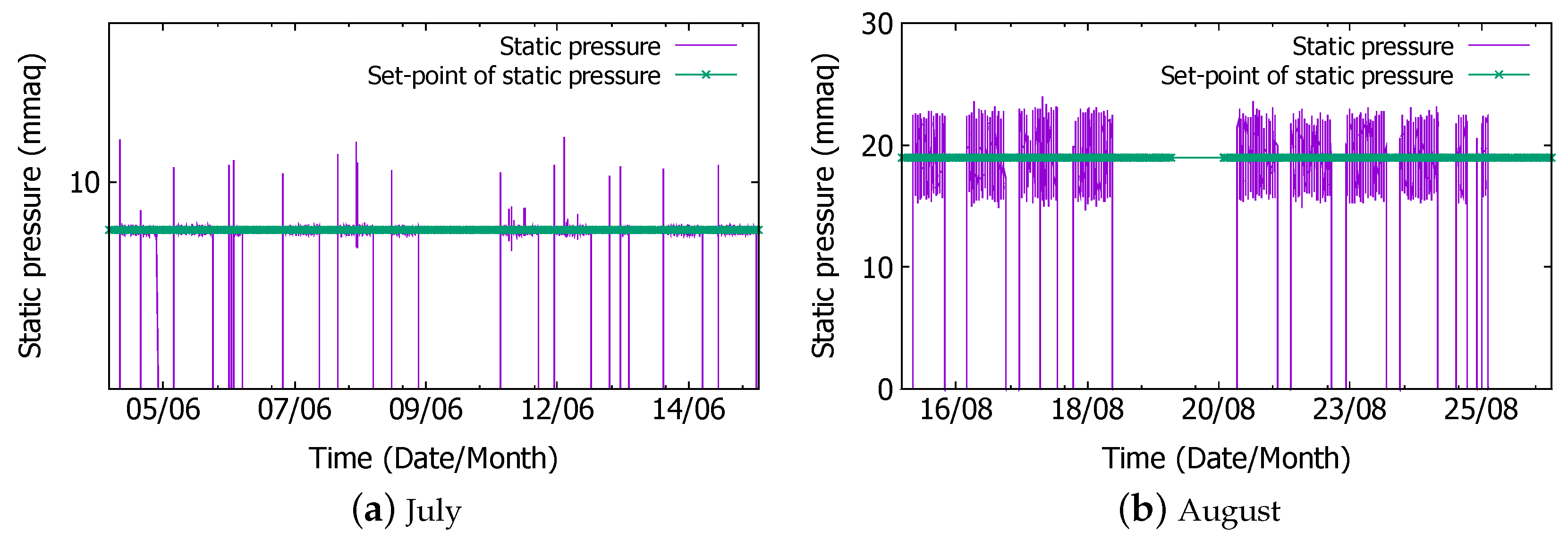
As mentioned before, our data sets have a distinctive feature. For the operational test during the summer break, we drove the system to the limits of the designed operating range. Since the time of the building construction, the ambient temperature may have changed from that used for the design. This operational test allowed us to re-estimate the required capacity and re-calibrate the set-points after the building was complete. As a result of the operational test conducted during the summer break, the static pressure after August 15 wildly fluctuates, which differs from the data acquired during normal operating conditions. Figure 6 compares the static pressures in the duct on the 4th floor in June and August. The graph on the left shows the static pressure sensor value in June when the static pressure set-point was fixed to 8 mmAq, whereas the graph on the right shows the data during the test of the HVAC system in August when the set-point of the static pressure was at 19 mmAq. Comparing the two graphs shows that the static pressure in June was stable, but the static pressure in August was unstable and fluctuated. The data from this abnormal operating condition were included in the training and test data to determine whether the model could predict the static pressure during such a test operation and whether the proposed model could replace the actual static pressure sensor in all anticipated operating situations.
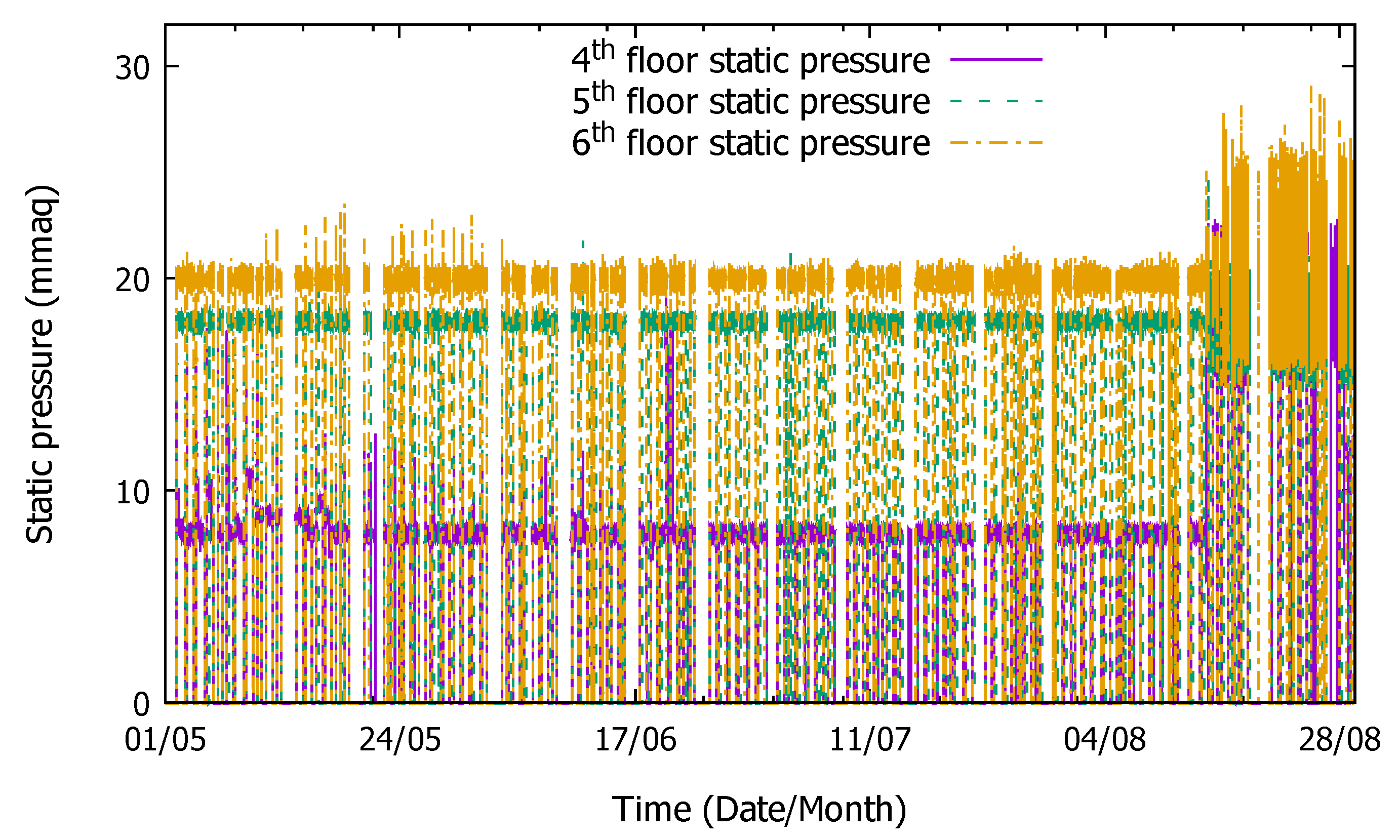
Figure 7 compares the static pressures of all data sets (4th, 5th, and 6th floors). Each floor had an HVAC system with different set-points, and the HVAC system tests were performed at all levels at about the same time in August. Since the designed static pressures are different on each floor, the measured static pressure ranges are different in this figure. We can also observe that, from 15 August to 29 August, the change in static pressure is unstable because of the test operation. We measured the predicted performance results of the LSTM model while changing the training and test data in the data sets for all three floors.

3.2. Proposed Deep Learning Model

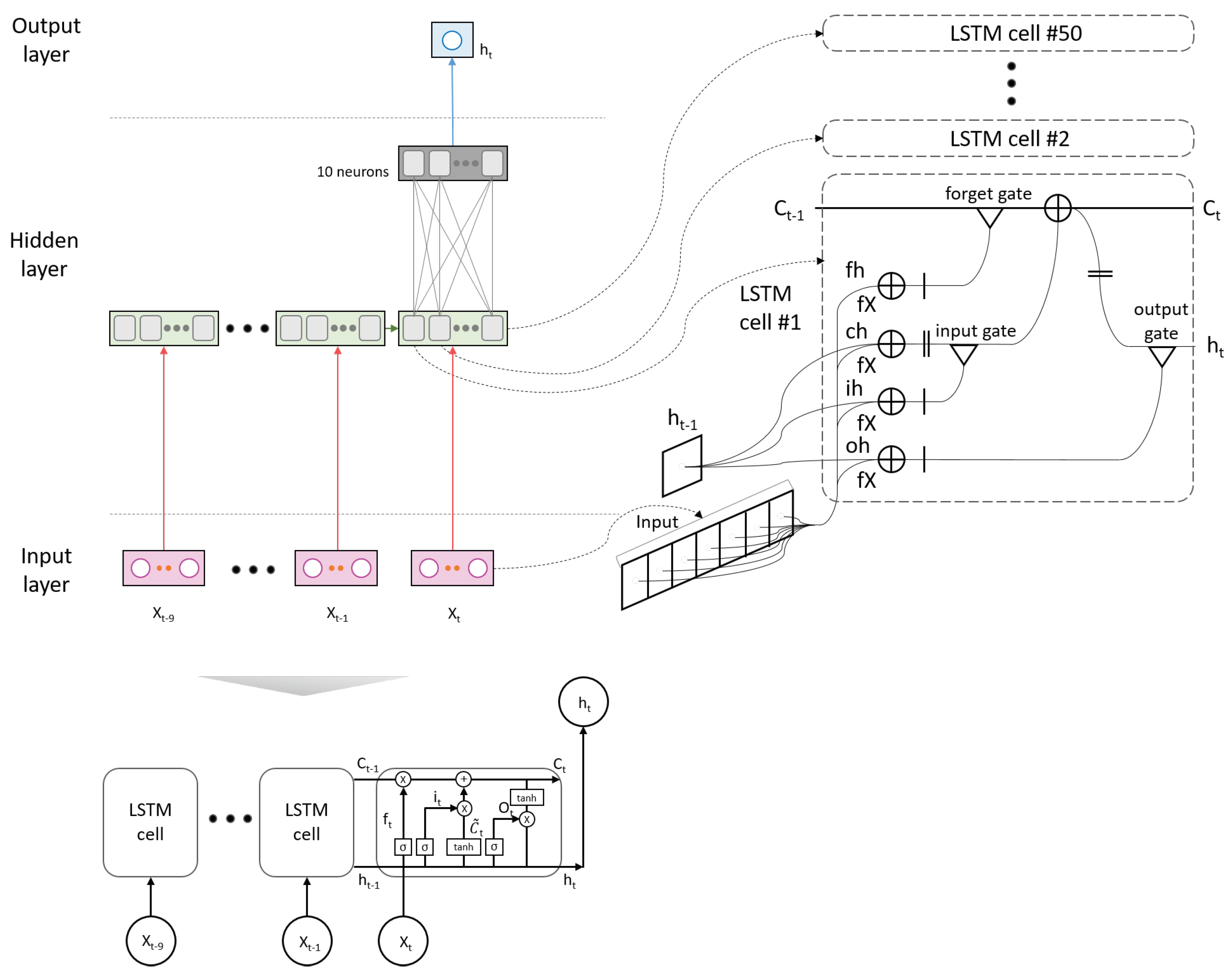
Among the deep learning techniques, the RNN (Recurrent Neural Network) is effective for learning sequential information. It recalls previous input from internal memory in the hidden layer to use with the input data in the subsequent data samples in the sequence. This feature makes it perfectly suited for machine learning problems that involve sequential data. Long Short-Term Memory (LSTM) is an extension for RNN that extends the memory to very long time lags. The memory in LSTM can be seen as a gated cell, and the gating is done by learning the importance of each input. Thus, LSTM can solve the long-term dependency problem by adding the cell state to the hidden state of the RNN. Time dependency is an important factor of learning time-series data characteristics. The experimental results with our data show that the best performance is achieved by using the previous nine data items. In other words, our LSTM model uses the data observed from the previous nine minutes to predict the data for the next minute. Therefore, of the different types of LSTM models, we used a many-to-one type (Figure 8) because our goal is to predict one next static pressure value from nine previous values. As described in Section 3.1, X t is a set of seven input parameters at time t, namely, the static pressure set-point, the temperature set-point, the volume of the supply air, the volume of the return air, the temperature of the supply air, the temperature of the return air, and the speed of the inverter fan.
In Figure 8, each LSTM cell has the following six functions:
f t = σ ( W X f X t + W h f h t 1 + b f ) ,
i t = σ ( W X i X t + W h i h t 1 + b i ) ,
C ˜ t 1 = t a n h ( W X g X t + W h g h t 1 + b g ) ,
C t = f t C t 1 + i t C ˜ t 1 ,
o t = σ ( W X o X t + W h o h t 1 + b o ) ,
h t = o t t a n h ( C t ) ,
where W denotes a weight factor, and b denotes bias for the gates in the LSTM cells. In Equations (1), (2) and (5), σ is a sigmoid layer used in the gates. It outputs numbers between 0 and 1 and determines how much of each information component should be let through the gate. For the forget gate f t in Equation (1), the sigmoid layer determines how much of the past information, which is stored in the form of the cell state, should be forgotten. The cell state facilitates the propagation of the gradient, even if the state is long in the LSTM. The forget logic looks at h t 1 , the output from the previous time step, and x t , the input at time step t, and outputs a number between 0 and 1 for each number in the cell state C t 1 . A sigmoid value of 1 means that the entirety of the given information should be kept, whereas 0 means that the entirety of the data should be forgotten. Next, the LSTM model decides what new information it will store in the cell state. First, the input gate i t decides which values it will update (Equation (2)). Second, a hypertangent (tanh) layer creates a vector of new candidate values C ˜ t to potentially add to the state (Equation (3)). Then, the LSTM updates the cell state in Equation (4). For this, the LSTM multiplies the old state C t 1 by f t using the Hadamard product ⊙, thereby forgetting the data according to its previous decision. Next, it adds i t C ˜ t 1 (Equation (4)). This is the new candidate value, scaled by how much it decided to update each state value. Finally, the LSTM model decides what to output. The output is based on the cell state but is a filtered version. First, a sigmoid layer decides what parts of the cell state it will output (Equation (5)). Then, it puts the cell state through tanh to squeeze the values so that they are between 1 and 1 and multiplies it by the output of the sigmoid gate. Thus, it outputs only the parts according to its previous decision (Equation (6)). Each input value ( X t ) is computed with the result predicted in the previous time step ( h t 1 ), and it passes through the input gate. It also controls the degree to which the previous learning value ( C t 1 ) affects the current learning by using the forget gate and the state value of the previously learned cell.

3.2.1. LSTM Network

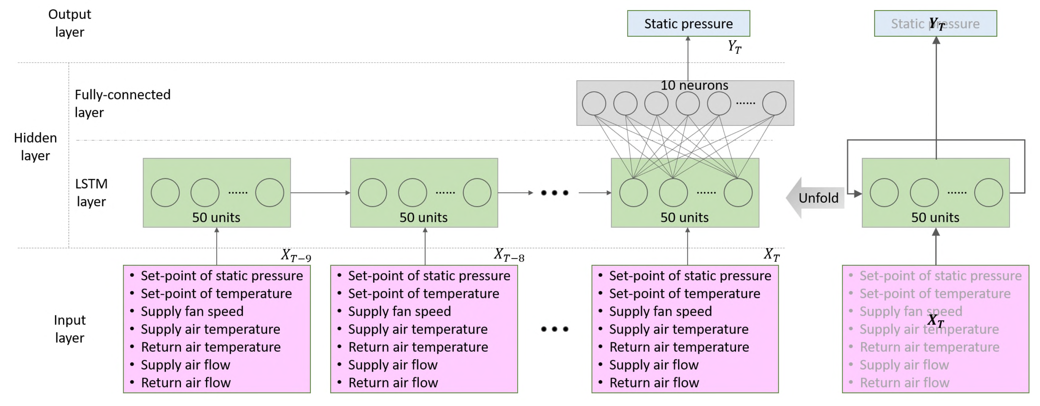
The entire LSTM network consists of input and output layers and two hidden layers, as shown in Figure 9, which is an unfolded representation. In the input layer, seven input samples at the current and the nine previous time steps, x t 9 , x t 8 , , x t 1 , x t , are applied.
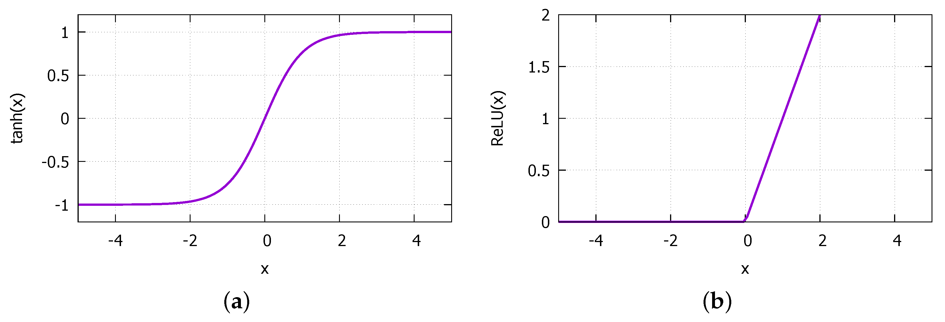
In other words, 10 previously measured sets of seven sample values are sequentially inputted in order to predict the next static pressure. The hidden layers consist of an LSTM layer and a fully connected layer. We found that the accuracy of the predicted static pressure value was higher when placing a fully connected layer between the LSTM layer and the output layer compared with directly connecting the 50 cells of the LSTM to the output layer. Similarly, the number of LSTM cells was selected empirically. When the number of cells is large, training takes longer, but, when it is small, the prediction accuracy is lower. For the activation functions, we employed the hypertangent (tanh) for the LSTM layer and the Rectified Linear Unit (ReLU) for the fully connected layer, as shown in Figure 10.
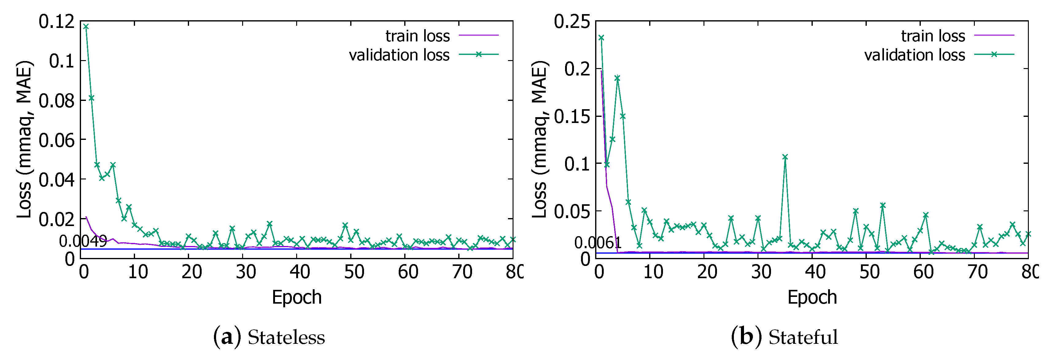
We used a stateless LSTM model. In a stateless model, the old state is memorized only by the batch size; if it is stateful, then the old learning contents are memorized throughout the learning process. As shown in Figure 11, in the stateful case, training and validation loss are no longer improved as the epoch continues. In the stateless case, the loss is slightly increased, but the performance is better than that in the stateful case because the loss decreases gradually. Thus, the stateless method is more effective for the static pressure prediction model than the stateful method for maintaining the learned contents throughout the learning process.

3.2.2. Hyperparameters

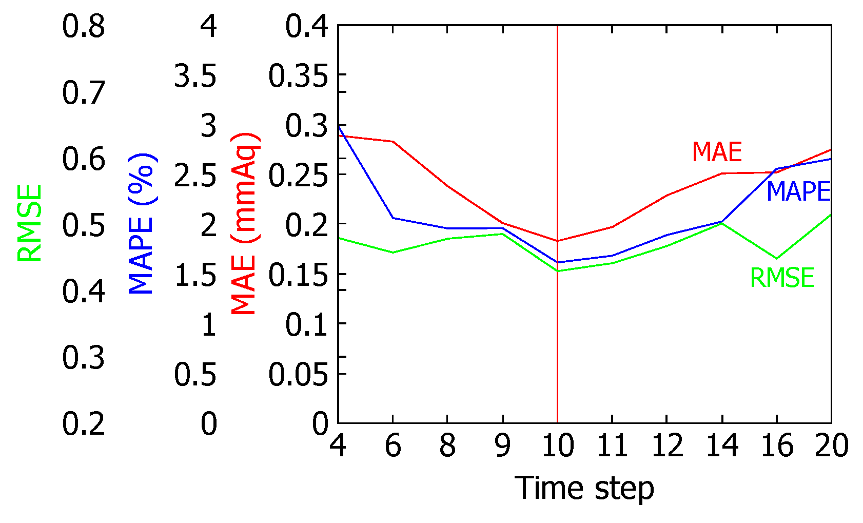
For prediction using time-series data, the interval of the data used for learning has a strong influence on the prediction result. If we use an interval that is too long or too short for learning, it is difficult to make accurate predictions. As shown in Figure 12, it can be seen that the error rate becomes larger based on the case where the timestep is 10. Because determining the number of time steps depends on the prediction application, we derived the optimal interval length for our application through experimental measurements.
Using metrics such as the Mean Absolute Error (MAE), Mean Absolute Percentage Error (MAPE), and Root Mean Square Error (RMSE)of the static pressure prediction while changing the time step, we observed that the error was frequently minimized at a time step size of 10. Table 1 shows our experiment with the time steps used for prediction. For a sampling interval of 1 min, the minimum error rate was achieved with 10 time steps. Therefore, in our model, a total of 10 time steps from t 9 to t min were used to predict the static pressure at time t.
Increases in the number of LSTM cells in the first hidden layer and the number of neurons in the second hidden layer increase only the learning time, and the accuracy of prediction does not improve. The early stopping method was used to prevent overfitting, and the batch size was selected to be 72, which produced the best error rates (Table 1). The MAE and Adam optimizer were used for the loss function and the training method, respectively. Table 2 shows the final selected hyperparameters.

4. Experimental Evaluation

The data sets from our HVAC system used for the proposed static pressure prediction were from three levels of an office building located in Seoul, Korea. Figure 13 shows the HVAC system configuration for the building. Except for the lobby (1st floor), the internal structures from the 2nd to the 6th floor are almost the same. The difference is that the HVAC systems on the 2nd and 3rd floors use a constant air volume, whereas the HVAC systems on the 4th and 6th floors use a variable air volume. The 1st, 2nd, and 3rd floors were designed as a public space for the lobby, library, and conference room, and all the installed HVAC systems use a constant air volume. This type of HVAC system does not control the speed of the fan according to the static pressure in the duct because it is operated with fixed speed fan speed. However, the 4th, 5th, and 6th floors are designed for use as offices and laboratories, and a variable-airflow HVAC system is installed because the heat load differs depending on the occupants and the conducted experiment. For a variable-airflow HVAC system, the fan speed must be controlled according to the static pressure in the duct, as described in Section 1.
The target building was built in January 2018, and the calibration of the HVAC facility and sensor values was carried out until April. After the residents moved in, the air volume was adjusted during the cooling/heating operation. Generally, the HVAC operational parameters of new buildings are adjusted for the spring, summer, and winter seasons for one year after the move-in. Therefore, in our experiment, the proposed deep learning model was developed and tested on the basis of the operational data from May to August. The reason that we used the data from this period is as follows. During spring (from March to May) and autumn (from September to November) in Korea, the HVAC system performs only the wind blowing operation. In summer (from June to August) and winter (from December to February), the cooling or the heating valve is opened for the cooling or heating operation, but, in these two seasons, the operation method for supplying the wind according to the set-temperature is the same. Therefore, in our experiment, the proposed model was developed and tested by using data from spring and summer (May–August) after the correction period ended in April. The model can also be used if the number of residents or usage purposes change between the design time and move-in. These changes can cause the air conditioning system to operate incorrectly. The operation test is performed to identify these changes and to set the optimal operating parameters using data such as user claims and the temperature and humidity inside the building. From 15 August to the end of August, the operation test was performed by the operator. During this time, the operation test was conducted while changing the set-point static pressure and the set-point temperature. In this study, we tested whether the proposed model could predict the static pressure during this period.
All input data items consist of the seven measured values defined in Section 3.1. As shown in Figure 9, we sequentially inputted data from the 10 previous time steps (from t 9 through t) to predict the static pressure and thereby estimate the static pressure at time step t. The training, validation, and test data periods used in each experiment are shown in Table 3.

4.1. Static Pressure Prediction in Normal and Test Operations

In order to validate our claim that DNN-based prediction of the static pressure in the duct is viable without installing and operating a pressure sensor, we performed the prediction using the LSTM network presented above and measured its accuracy by comparing its predictions with the sensor data. For training and testing, we used all three data sets from different floors of the target building. In Experiment 4.1 in Table 3, we divided each data set of three floors into training, validation, and test data by month. The total number of data entries in the 4th floor data set was 172,206 after removing faulty or lost data entries. Among these data points, 125,120 were used for the training and validation, and 47,086 were used to test the model. In the 5th floor data set, the total number was 172,186, of which 126,656 were used for training and validation, and 45,530 were used for testing. In the 6th floor data set, the total was 171,933, with 126,470 used as the training and validation data, and 45,463 used as the test data.
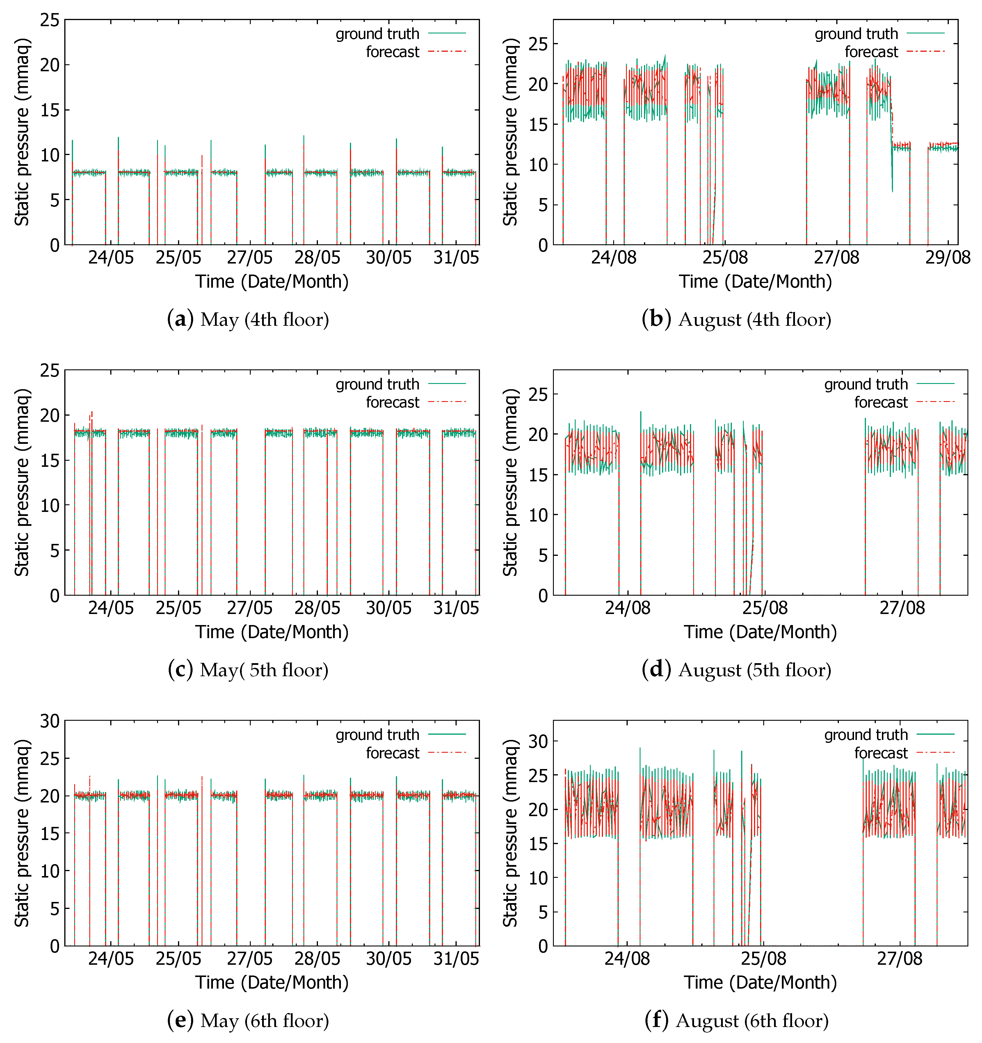
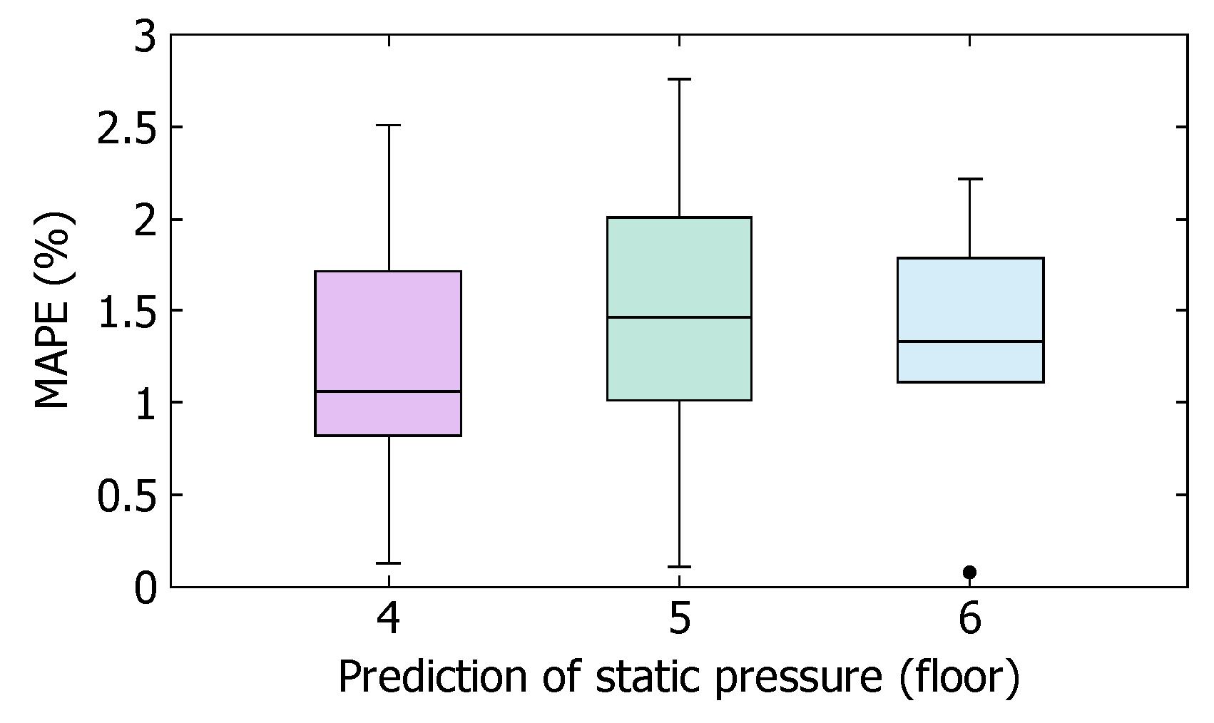
The result of the test on the 4th floor data set is encouraging, with MAE = 0.139 mmAq, MAPE = 1.064%, and RMSE = 0.398. This error is safely within the 5–10% error margin recommended by the ASHREA standard [26]. Figure 14 graphically shows how close the predicted values are to the sensed values. In the figures, the left column is for May, during which the system was in regular operation. The right column corresponds to the test operation during August, which is in the summer vacation season. In Figure 14a, the set-point was constant at 8 mmAq, and we can see that the prediction closely matches the sensed static pressure. For the 5th floor, the target static pressure was set at 16 mmAq. In this experiment, the LSTM model for each floor was trained with the data from that particular floor. Nonetheless, the prediction by the LSTM network has similar precision: MAE = 0.222 mmAq, MAPE = 1.464%, and RMSE = 0.498 for May (Figure 14c). For the 6th floor, MAE = 0.234 mmAq, MAPE = 1.333%, and RMSE = 0.471 for May (Figure 14e). The prediction error distribution for each floor is shown in Figure 15.
In Figure 14b, however, the static pressure significantly fluctuates because the system was operated at the extremes of the designed operating range. In the designed operating ranges, the static pressure should be kept under 15 mmAq for the 4th floor, 20 mmAq for the 5th floor, and 30 mmAq for the 6th floor. In any condition, the static pressures for these floors should never exceed 40 mmAq.
Even for the recalibration operation that pushes the system to this limit, the prediction by the LSTM network trained with the values produced from August 1 to 22 matches the real values relatively well. The error figures for the 4th floor during the recalibration period are MAE = 0.317 mmAq, MAPE = 2.941%, and RMSE = 0.968. Again, we obtained similar error values to those from the other floors. For the 5th floor, the static pressure fluctuates wildly (Figure 14d), which leads to slightly larger errors: MAE = 0.409 mmAq, MAPE = 3.284%, and RMSE = 1.391. For the 6th floor, MAE = 0.398 mmAq, MAPE = 4.319%, and RMSE = 1.173 (Figure 14f).
The test results for each floor clearly show that the proposed model produces values that are close to the sensor-measured ones. The precision holds regardless of the operation mode (normal or operational test), and we can predict the real pressure without a pressure sensor in the duct as long as the training data are provided to the LSTM network. Even the more wildly fluctuating values during the operational tests are well predicted.
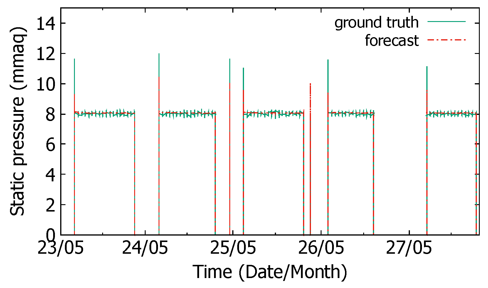
One more interesting point in the predicted pressure in Figure 14 is that the model can even detect transient behaviors of the modeled system. In Figure 14a,c,e, the static pressure rises momentarily upon the initial start-up of the system on a given day. Figure 16 shows a more detailed figure that shows spikes at the start-up times. When the HVAC system is in operation, the static pressure on the duct rises momentarily because the pressure of the air that is blown when the fan is first started is applied to the duct, and the fan is operated to adjust the speed again on the basis of the static pressure. The LSTM-based model can predict even this momentary rise in static pressure.

4.2. Static Pressure Prediction for Untrained Seasons

We further explored the power of the LSTM-based predictor for forecasting values in different seasons for which it was not trained. In general, HVAC systems operate for heating in winter and cooling in summer, while they simply blow air in spring and autumn. In this experiment, we tested whether the prediction model trained by the spring (May) data could predict the static pressure during the cooling operation in summer (July and August) for the 4th floor. The importance of this experiment is that we are testing the prediction performance when the cooling valve is open using the trained model without cooling or heating. Since the winter operation is different from the summer operation only in terms of the set-point temperature, we do not need to test our model against the winter data. For this experiment, we used 44,567 samples from May for training. Then, for the out-of-season test, we used 44,635 data samples from July and 39,805 data samples from August.
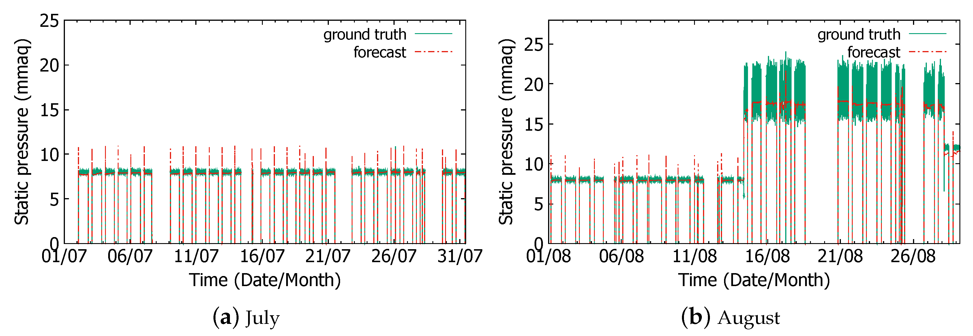
The LSTM-based prediction model trained by the May data produces results for July with MAE = 0.084 mmAq, MAPE = 1.115%, and RMSE = 0.184. Figure 17 shows that the LSTM prediction closely matches the ground truth given by the July data, except for some spikes at the start of the operation every day. Even though the air-cooling operation was performed in July, these two months both use a constant set-point for the static pressure. On the other hand, the results for August are again relatively less accurate as a result of the test operation, which pushed the system to the designed operating range limits. In August, the set-point was 19, which is much larger than the set-point of 9 used in the other months.
The error values for August are an MAE of 0.617 mmAq, MAPE of 3.876%, and RMSE of 1.448. Considering the large variability in August, however, even this prediction result is not completely off the mark. In Figure 17a, when the HVAC system operation is in the normal state, the static pressure in the duct remains at its set value. However, as shown in Figure 17b, the system operation is at the extremes of the designed range, and the static pressure in the duct is highly unstable. Even in this case, however, the LSTM-based predictor outputs stable values within the fluctuating range (15–18 mmAq). Recall that this result is obtained despite the lack of such highly fluctuating data in August. If these data were provided, as we observe in Section 4.1, these wild fluctuations can be predicted with even more precision, with MAE = 0.317 mmAq, MAPE = 2.941%, and RMSE = 0.968.

4.3. Static Pressure Prediction in Operations with Different Capacity

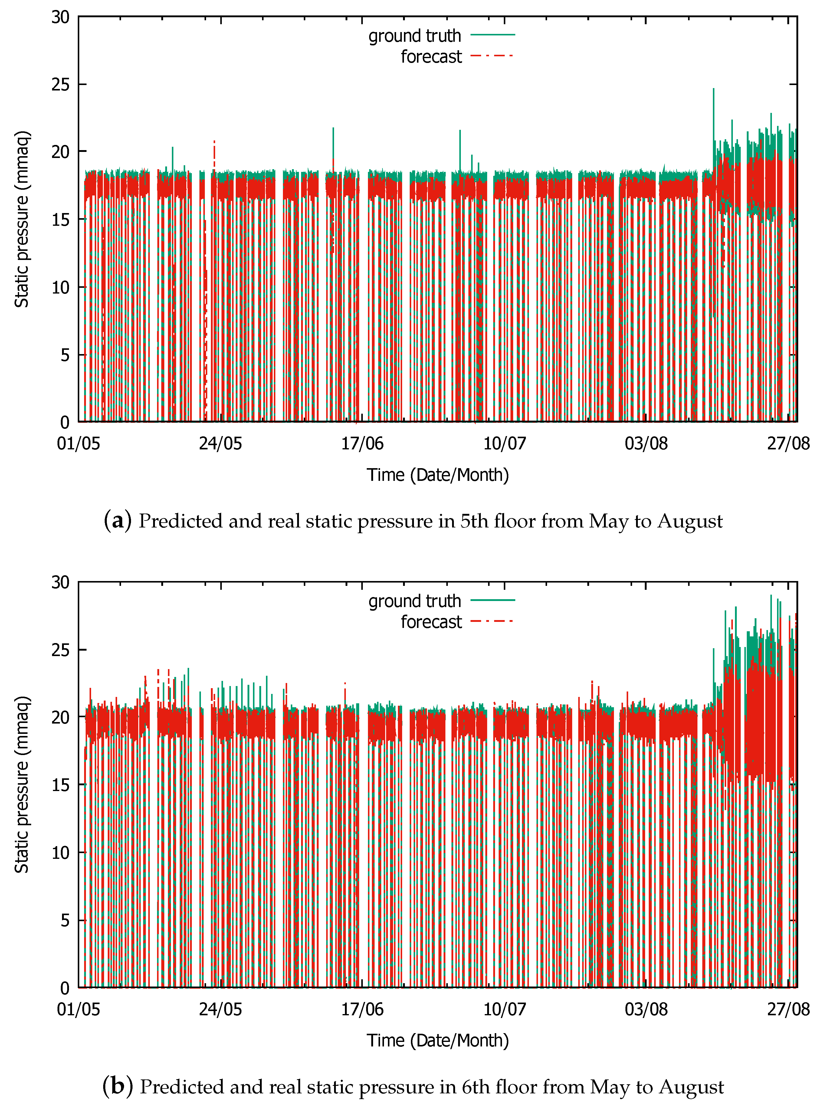
To further explore the performance of the LSTM-based predictor on untrained data, we tested the model trained on data from 4th, 5th, and 6th floors. These floors require HVAC systems with the same configuration but different heat loads. The data from May to August on the 4th floor were used as learning data, and the static pressures on the other two floors were predicted. The input data from the 4th floor system consisted of 172,205 samples, and the test data from the 5th and 6th floors were 172,186 and 171,933, respectively. Note that the test data are all the data from the 5th and 6th floors.
The predicted results for the static pressure on the 5th floor are 0.298 mmAq for MAE, 1.964% for MAPE, and 0.898 for RMSE. The error characteristics are not as good as those for the 4th floor, but it is a surprisingly good result considering that the set-point static pressure on the 5th floor is 18 mmAq, which is twice that on the 4th floor. The result for the 6th floor is similar, with an MAE of 0.313 mmAq, MAPE of 2.062%, and RMSE of 0.954. The set-point static pressure on the 6th floor was even higher at 20 mmAq, but the model trained on the 4th data worked relatively well for the other floors. Figure 18 graphically compares the prediction and the real values measured by the sensors from May to July and the test period in August. For this experiment, we used the test period data from the 4th floor in August. When the data are available, the static pressure for other floors with different capacities can be predicted.
This result implies that, when the data from an AHU are not available, we can use those from other floors and create a trained model as a rough initial predictor. Then, as the data are obtained, we can train for the AHU to refine the model.

4.4. Prediction of Data with Different Time Intervals

In prediction techniques that use time-series data, the period of data used for learning is an important factor to consider when creating and optimizing a model. As mentioned in Section 3.2.2, the proposed model has the best prediction results when the time step is 10. However, if the data used for learning are at 5-min intervals instead of 1 min, as in the data currently used, then the time step is the most important component of the proposed model. We applied the May data from the 4th floor to the proposed model at intervals of 5 min. In contrast to the 1-min interval data, a time-step of 3 is most suitable (see Table 4). The error rate is slightly higher in a test of the same period because the data at the interval of 5 min decreased the accuracy of the static pressure value prediction. We also tested changes in the LSTM cells, but they did not significantly affect the results.

5. Conclusions and Future Work

In this paper, we demonstrate that a deep learning-based approach can eliminate the need for static pressure sensors in part of the HVAC system. We used an LSTM-based model that learns the time-series characteristics of the static pressure in the HVAC system so that we can eliminate the static pressure sensor from the system. We experimentally verified that the proposed model could precisely match the static pressure measured by the sensor, regardless of seasonal characteristics and HVAC system capacity. This method allows us to reduce the investment cost of the sensor for operating the HVAC system. Thus, it is technically possible to replace the hardware with intelligent software.
However, the proposed model can not be applied to HVAC systems using more than two static pressure sensors. In this case, we need to develop a new sophisticated model because the main duct is branched and the static pressure sensor is installed for each duct.
We believe that, by extending the proposed model, the HVAC system control method can be made more intelligent. First, we think that the prediction model can be trained to detect the malfunction of the system if a dataset is used that includes malfunction events. Second, we think that the fan control method can be trained through reinforcement learning according to the predicted static pressure. More stable fan control will reduce the energy consumption of the equipment and can yield additional benefits by preventing failures.

Author Contributions

H.K. conceived and designed the experiments; J.S. performed the experiments and analyzed the data; H.K. wrote the paper.

Funding

This work was supported by the Korea Institute of Energy Technology Evaluation and Planning (KETEP) and the Ministry of Trade, Industry and Energy (MOTIE) of the Republic of Korea (No. 20188550000410).

Conflicts of Interest

The authors declare no conflict of interest. The founding sponsors had no role in the design of the study; in the collection, analyses, or interpretation of data; in the writing of the manuscript, and in the decision to publish the results.

References

  1. IBM Research Editorial Staff. IoT and Machine Learning to Reduce Energy Use in Cooling Systems. Available online: https://www.ibm.com/blogs/research/2018/07/reduce-energy-cooling/ (accessed on 10 January 2018).
  2. Ahmad, M.W.; Mourshed, M.; Yuce, B.; Rezgui, Y. Computational intelligence techniques for HVAC systems: A review. Build. Simul. 2016, 9, 359–398. [Google Scholar] [CrossRef] [Green Version]
  3. Li, X.; Zhao, T.; Fan, P.; Zhang, J. Rule-based fuzzy control method for static pressure reset using improved Mamdani model in VAV systems. J. Build. Eng. 2019, 22, 192–199. [Google Scholar] [CrossRef]
  4. Ethan, P.; Seshadhri, S.; Korkut, B.; Jiang, C.; Rong, S.; Kameshwar, P. An internet of things upgrade for smart and scalable heating, ventilation and air-conditioning control in commercial buildings. Appl. Energy 2019, 239, 408–424. [Google Scholar]
  5. Shahnazari, H.; Mhaskar, P.; House, J.M.; Salsbury, T.I. Modeling and fault diagnosis design for HVAC systems using recurrent neural networks. Comput. Chem. Eng. 2019, 126, 189–203. [Google Scholar] [CrossRef]
  6. Reynolds, J.; Ahmad, M.W.; Rezgui, Y.; Hippolyte, J.L. Operational supply and demand optimisation of a multi-vector district energy system using artificial neural networks and a genetic algorithm. Appl. Energy 2019, 235, 699–713. [Google Scholar] [CrossRef]
  7. Iqbal, R.; Maniak, T.; Doctor, F.; Karyotis, C. Fault Detection and Isolation in Industrial Processes Using Deep Learning Approaches. IEEE Trans. Ind. Inform. 2019, 9, 359–398. [Google Scholar] [CrossRef]
  8. Jantscher, P. AI in Sensors for IoT. Available online: https://siliconsemiconductor.net/article/106227/AI_In_Sensors_For_IoT (accessed on 28 January 2019).
  9. Carrier Design Manual Part 2: Air Distribution, 10th ed.; Carrier Corporation: Farmington, CT, USA, 1960.
  10. Kato, K.; Sakawa, M.; Ishimaru, K.; Ushiro, S.; Shibano, T. Heat load prediction through recurrent neural network in district heating and cooling systems. In Proceedings of the 2008 IEEE International Conference on Systems, Man and Cybernetics, Singapore, 12–15 October 2008; pp. 1401–1406. [Google Scholar]
  11. Vázquez-Canteli, J.R.; Ulyanin, S.; Kämpf, J.; Nagy, Z. Fusing TensorFlow with building energy simulation for intelligent energy management in smart cities. Sustain. Cities Soc. 2019, 45, 243–257. [Google Scholar] [CrossRef]
  12. Park, J.Y.; Dougherty, T.; Fritz, H.; Nagy, Z. LightLearn: An adaptive and occupant centered controller for lighting based on reinforcement learning. Build. Environ. 2019, 147, 397–414. [Google Scholar] [CrossRef]
  13. Papadopoulos, S.; Kontokosta, C.E.; Vlachokostas, A.; Azar, E. Rethinking HVAC temperature set-points in commercial buildings: The potential for zero-cost energy savings and comfort improvement in different climates. Build. Environ. 2019, 155, 350–359. [Google Scholar] [CrossRef]
  14. Valladares, W.; Galindo, M.; Gutierrez, J.; Wu, W.-C.; Liao, K.-K.; Liao, J.-C.; Liu, K.-C.; Wang, C.-C. Energy optimization associated with thermal comfort and indoor air control via a deep reinforcement learning algorithm. Build. Environ. 2019, 155, 105–117. [Google Scholar] [CrossRef]
  15. Jackson, D.A. Stopping rules in principal components analysis: A comparison of heuristical and statistical approaches. Ecology 1993, 74, 2204–2214. [Google Scholar] [CrossRef]
  16. Lee, K.P.; Wu, B.H.; Peng, S.L. Deep-learning-based fault detection and diagnosis of air-handling units. Build. Environ. 2019, 157, 24–33. [Google Scholar] [CrossRef]
  17. Guo, Y.; Tan, Z.; Chen, H.; Li, G.; Wang, J.; Huang, R.; Liu, J.; Ahmad, T. Deep learning-based fault diagnosis of variable refrigerant flow air-conditioning system for building energy saving. Appl. Energy 2018, 225, 732–745. [Google Scholar] [CrossRef]
  18. Consoli, A.; Scarcella, G.; Testa, A. Industry application of zero-speed sensorless control techniques for PM synchronous motors. IEEE Trans. Ind. Appl. 2001, 37, 513–521. [Google Scholar] [CrossRef]
  19. Maes, J.; Melkebeek, J.A. Speed-sensorless direct torque control of induction motors using an adaptive flux observer. IEEE Trans. Ind. Appl. 2000, 36, 778–785. [Google Scholar] [CrossRef]
  20. Kim, T.H.; Ehsani, M. Sensorless control of the BLDC motors from near-zero to high speeds. IEEE Trans. Power Electron. 2004, 19, 1635–1645. [Google Scholar] [CrossRef]
  21. Yilmaz, M.; Tuncay, R.N.; Ustun, O.; Krein, T.P. Sensorless Control of Brushless DC Motor Based on Wavelet Theory. Electr. Power Compon. Syst. 2009, 37, 1063–1080. [Google Scholar] [CrossRef]
  22. Hirose, N.; Tajima, R. Modeling of rolling friction by recurrent neural network using LSTM. In Proceedings of the 2017 IEEE International Conference on Robotics and Automation (ICRA), Singapore, 29 May–3 June 2017; pp. 6471–6478. [Google Scholar] [CrossRef]
  23. Shamshirband, S.; Petković, D.; Anuar, N.B.; Kiah, M.L.M.; Akib, S.; Gani, A.; Ćojbašićb, Ž.; Nikolić, V. Sensorless estimation of wind speed by adaptive neuro-fuzzy methodology. Int. J. Electr. Power Energy Syst. 2014, 62, 490–495. [Google Scholar] [CrossRef]
  24. Nikolić, V.; Motamedi, S.; Shamshirband, S.; Petković, D.; Ch, S.; Arif, M. Extreme learning machine approach for sensorless wind speed estimation. Mechatronics 2016, 34, 78–83. [Google Scholar] [CrossRef]
  25. Kumar, R.; Sivashanmugam, P. Neuro and Fuzzy Computing Approach for the Flow Sensorless Measurement. Sens. Transducers 2009, 109, 21. [Google Scholar]
  26. Measurement, Testing, Adjusting, and Balancing of Building HVAC Systems. In ANSI/ASHRAE Standard 111-2008; ASHRAE: New York, NY, USA, 2008.
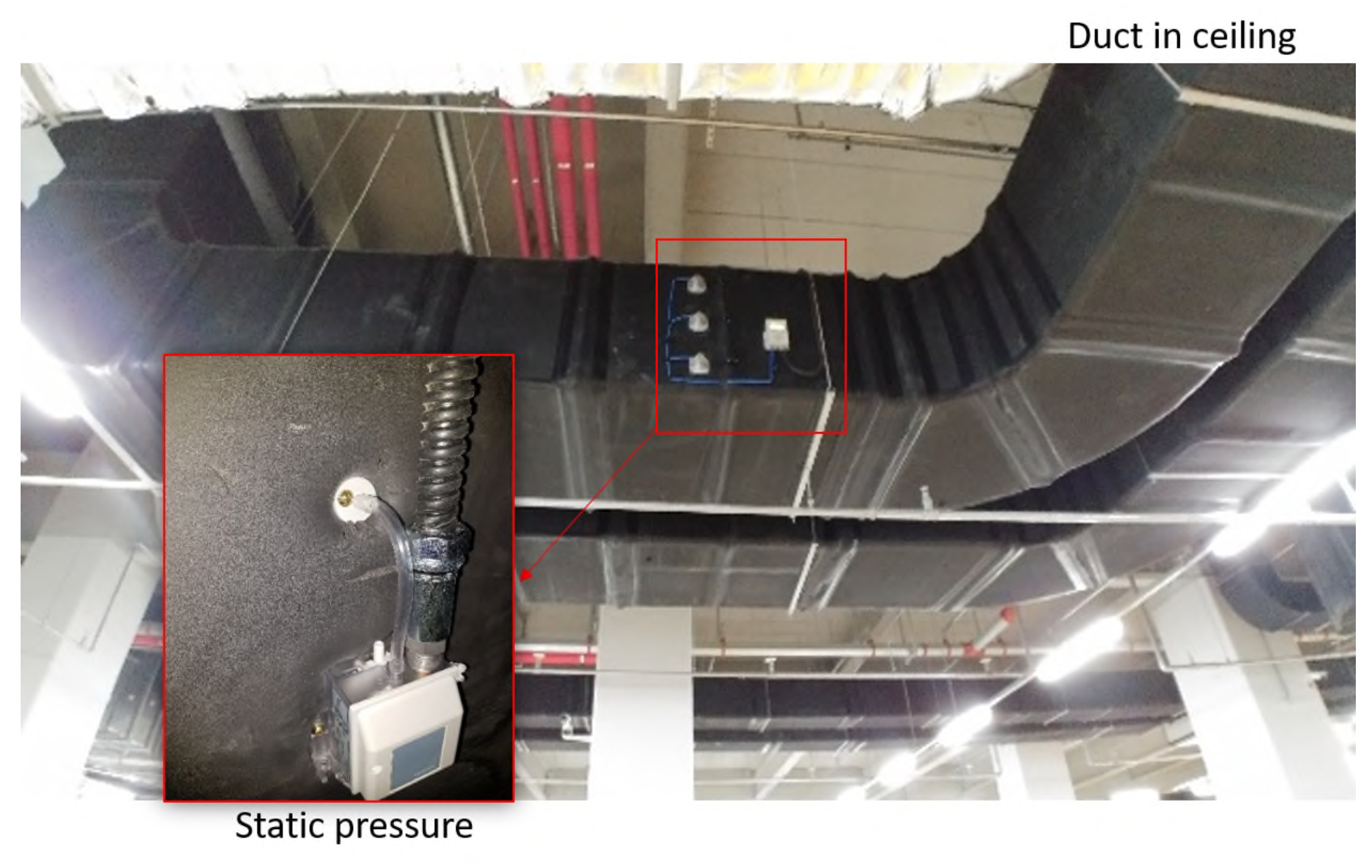
Figure 1. Duct and installed static pressure sensor.
Applsci 09 03293 g001
Figure 2. Air flow between the Air Handling Unit (AHU) and the room.
Applsci 09 03293 g002
Figure 3. Training and testing process used in this paper.
Applsci 09 03293 g003
Figure 4. Air Handling Unit (AHU) and the connected components in the system.
Applsci 09 03293 g004
Figure 5. The 4th floor data set.
Applsci 09 03293 g005
Figure 6. Comparison of static pressure.
Applsci 09 03293 g006
Figure 7. Comparison of static pressure of each floor.
Applsci 09 03293 g007
Figure 8. Our Long Short-Term Memory (LSTM) structure for the sensorless system.
Applsci 09 03293 g008
Figure 9. Deep learning structure for forecasting static pressure in ducts.
Applsci 09 03293 g009
Figure 10. Activation functions: (a) hypertangent (tanh) used for hidden layers; (b) rectified linear unit (ReLU) activation function used for the output layer.
Applsci 09 03293 g010
Figure 11. Loss of train and validation.
Applsci 09 03293 g011
Figure 12. Prediction performance by time step.
Applsci 09 03293 g012
Figure 13. Heating, Ventilation, and Air Conditioning (HVAC) system structure of target building.
Applsci 09 03293 g013
Figure 14. Forecast results for May and August of each floor.
Applsci 09 03293 g014
Figure 15. Distribution of prediction error.
Applsci 09 03293 g015
Figure 16. The LSTM-based predictor even catches the momentary spikes at the start of fan operation.
Applsci 09 03293 g016
Figure 17. Out-of-season forecast results of the LSTM-based predictor trained using data from May.
Applsci 09 03293 g017
Figure 18. Forecast results for HVAC systems on different floors.
Applsci 09 03293 g018
Table 1. Prediction performance with 1-min time steps.
Time StepUnits of LSTMBatch SizeMAEMAPERMSE
1050360.1971.7150.451
720.1941.6980.433
1280.2181.9620.487
100720.1951.7110.425
50 × 24720.1821.6080.421
Table 2. The parameter setting detail of the proposed model.
OptionParameter Setting
Batch size72
Time step10
Training stop strategyEarly stopping
Loss functionMAE (Mean Absolute Error)
Training methodAdam optimizer
Table 3. Training, validation and test data period for each experiment.
ExperimentTraining DataValidation DataTest Data
4.1 (4F, 5F, 6F)01/05–17/05 (17 days)18/05–22/05 (5 days)23/05–31/05 (9 days)
01/06–18/06 (18 days)19/06–22/06 (4 days)23/06–30/06 (8 days)
01/07–17/07 (18 days)18/07–22/07 (5 days)23/07–31/07 (9 days)
01/08–17/08 (17 days)18/08–20/08 (3 days)21/08–29/08 (9 days): 4F
21/08–28/08 (8 days): 5F, 6F
4.2 (4F)01/05–25/05 (25 days)26/05–31/05 (6 days)01/07–29/08 (60 days)
4.301/05–25/05 (25 days)26/05–31/05 (6 days)01/05–28/08 (120 days): 5F, 6F
01/06–24/06 (24 days)25/06–30/06 (6 days)
01/07–25/07 (25 days)26/07–31/07 (6 days)
01/08–24/08 (24 days)25/08–29/08 (5 days)
Table 4. Prediction performance over time steps.
Time StepUnitMAEMAPERMSE
1501.2898.2412.628
2500.8015.6511.958
1000.7915.3121.799
3500.3181.9650.782
4500.2751.3270.574
1000.2591.5750.580
5500.3021.6790.694
7500.4943.0651.221
10501.0077.1152.571
12501.0257.5262.598