Article

A Method of Path Planning on Safe Depth for Unmanned Surface Vehicles Based on Hydrodynamic Analysis

1
School of Marine Science and Technology, Tianjin University, Tianjin 300072, China
2
Tianjin Port Environmental Monitoring Engineering Center, Tianjin 300072, China
*
Authors to whom correspondence should be addressed.
Appl. Sci. 2019, 9(16), 3228; https://doi.org/10.3390/app9163228
Submission received: 30 June 2019 / Revised: 25 July 2019 / Accepted: 31 July 2019 / Published: 7 August 2019
(This article belongs to the Special Issue Mobile Robots Navigation)

Abstract

:
The depth of water is of great significance to the safe navigation of unmanned surface vehicles (USV)in shallow waters, such as islands and reefs. How to consider the influence of depth on the safety of USV navigation and path planning is relatively rare. Under the condition of ocean disturbance, the hydrodynamic characteristics of unmanned surface vehicles will affect its draft and depth safety. In this paper, the hydrodynamic model of unmanned surface vehicles is analyzed, and a water depth risk level A* algorithm (WDRLA*) is proposed. According to the depth point of the electronic navigation chart (ENC), the gridding depth can be obtained by spline function interpolation. The WDRLA* algorithm is applied to plan the path, which takes hydrodynamic characteristics and navigation errors into account. It is compared with the traditional A* shortest path and safest path. The simulation results show that the WDRLA* algorithm can reduce the depth hazard of the shortest path and ensure the safety of navigation.

1. Introduction

As a sort of autonomous ocean vehicles, USV (unmanned surface vehicles) can autonomously perform tasks in various environments without human intervention [1]. USV with non-linear dynamic characteristics have better endurance ability and payload ability than other unmanned vehicles, which makes them to be essential tools in the area of marine scientific research, marine resources development, marine environment monitoring and national marine security [2,3,4]. Autonomy and intellectualization are the crucial manifestations of the development of USV. Research on intelligent planning and controlling can improve the working performance of USV [5].
In the area of intelligent planning and control, path planning of single objectives, such as shortest distance, time optimality, energy consumption optimality, smoothness optimality and minimal risk, has gradually been studied furtherly [6]. Multi-objective motion planning and intelligent decision-making [7,8] considering dynamic constraints of mobile robots is the difficulty of current research, where it is necessary to obtain more comprehensive and accurate environmental information by using environmental comprehensive perception methods, such as maps to optimize the path planning results. In this context, it is of great significance to study the path planning algorithm based on ENC (electronic navigation chart) considering the hydrodynamic characteristics of USVs for improving the USV’s autonomous environmental awareness, optimizing the path planning results and improving the autonomy and intelligence level of USVs.
A star algorithm, (A* algorithm) is a deterministic algorithm with outstanding consistency and completeness which is widely applied in the research of path planning. It was firstly proposed by Hart P. et al. [9] and usually combined with grid method [10]. The minimum cost function is used to search the minimum cost path from the starting node to the end node. The grid-based A* path search methods are mainly based on the center point of the grid [11,12,13,14,15,16] and grid vertexes [7,10,17,18,19]. Grid method can be divided into a uniform grid and non-uniform grid with diverse shapes and sizes of the grid. Aiming at the deficiencies of the grid-based A* algorithm, such as huge memory expenditure, large path turning angle and unsmooth path, studies have been done to improve it.
Larson et al. [20] found the optimal path with the least nodes in limited time by using A*. Svec et al. [21] combined the A* and locally bounded plan, Naeem et al. [22] proved A* by direction priority sequential selection (DPSS), Improving path quality and computational capacity. Svec et al. [23] introduced a model prediction algorithm and combined it with A* algorithm. The above work concentrates on improving the computational performance and path quality of traditional A* algorithm.
Daniel, K [16] and Soulignac, M [24] carried out the Theta* which released the limited that the center points of the grid can only moves along the center points within A*. Kim et al. [13] solved the problem of unlimited direction with the theory of limit-cycle circle set. Nash, A et al. [15] carried out Lazy Theta*, it was found that vertexes visibility check decreases by using this method. Improved dynamic search D* was put forward by Yang, J.M. et al. [17] based on A*, it was demonstrated that this algorithm fits the dynamic map very well.
Wu, P.P et al. [7] carried out a multi-objective A*, it improves the real-time performance of A*. Naus et al. [25] applied A* to search the shortest and safest trajectory in electronic chart. Kim et al. [26] carried out a curvature path planning algorithm which considering the turning ability of USV through perfecting A*. Liu, C.G. et al. [18] established the surface obstacles risk model considering current, traffic separation and maneuverability and improved the practicability of A* algorithm, but ignored the effect of water depth on navigation safety. In the above work, the A* algorithm is applied to the area of path planning for USVs.
Previous researches perfected the calculating quality of A* and expanded the range where A* could be involved in, and they focused on the estimation of the criticality of surface obstacles in the research concerning safest path planning of USVs, rarely discussed the hazard, due to the shallow depth. Depth is a crucial factor affecting navigation safety and performance for unmanned surface vehicles operation in shallow waters, which is more vulnerable to ocean disturbances, such as wind, waves and currents, [27]. On the other hand, the hydrodynamic characteristics can well reveal the navigation stability of small USVs in shallow waters [28,29], and then evaluate the safe depth of navigation.
In this paper, a method of safe path planning is carried out to improve the depth safety of the shortest path of USV, which guarantees navigation safety in different conditions. In this paper, the navigation stability of USVs in various situations is studied, and the minimum safe water depth is calculated according to the results of hydrodynamics simulation. On this basis, the safer path of USVs is calculated by considering the risk of water depth. The depth safety of USV, which followed the shortest path, could be improved by using the information of depth in ENC, the water depth risk level (WDRL) of shortest path could be reduced as well.

2. Modeling

2.1. Hydrodynamic Modeling

Small unmanned surface vehicles are insufficient to resisting wind and waves. When sailing in constrained waters, due to the blockage effect of water boundary, the reflected wave and the generated wave of the boundary overlap or decrease each other, which results in pressure distribution difference on the hull surface, generating heave and trim motion and deducing sticking on bottom, shore touching and capsizing of the vessel and endangering the safety of navigation. Our group has developed an unmanned surface vessel with an adjustable scale shown as Figure 1 and Table 1 for marine surveying and mapping. The hull is made of two inflatable protons. The width of the equipment bracket can be adjusted and quickly disassembled/assembled in 30 minutes. The navigation status of this unmanned surface vehicle is studied with three kinds of velocity in irregular waves as an example, and then the criticality of the draft variation is estimated. The parameters of the USV are as follows:
The ship’s navigation status mainly contains three states: Heave, pitch and speed. Nine cases were set up with three speeds (5 kn, 8 kn, 11 kn) and three wave heights (0.5 m, 1 m, 1.5 m) when wave period is 2 s (shown in Table 2).
The governing equations were solved by RANS (standard k-ε) with STAR-CCM+. Assuming that the fluid flow is viscous and incompressible, the governing equations are established as below:
div u = 0 ,
u t + div ( u u ) = 1 ρ p x + v div ( grad u ) ,
v t + div ( vu ) = 1 ρ p y + v div ( grad v ) ,
w t + div ( wu ) = 1 ρ p z + v div ( grad w ) ,
where u, v, w are respectively the components of velocity on the directions of x, y, z (see Figure 1).
The waves were generated by Pierson-Moskowitz spectra, which defines the motion of irregular waves—it is written as:
S P M ( ω ) = 5 16 ( H S 2 ω P 4 ) ω 5 exp ( 5 4 ( ω ω P ) 4 ) ,
where ω is the angular frequency of waves. ω P = ( 2 π ) / ( T P ) represents the peak frequency of the spectrum. T P is the peak wave period. H S is significant wave height (m).
The velocity distribution of the flexible wave generator plate is employed to generate a simulated incident, waves at the inlet boundary, the wave surface equation of irregular waves can be expressed as follows:
η = H s cos ( m x ω t ) ,
in which η is energy, and m is the number of waves. The velocity field of irregular wave is as below:
{ U = ω H e k z cos ( m x ω t ) V = 0 W = ω H e k z sin ( m x ω t ) ,
where U and W are velocity profiles on x and z direction. H is the wave amplitude, k is wave-number (2π/m). x-axis is the direction of wave propagation, and the z-axis is the direction of wave fluctuation. The wave propagation direction is parallel to the heading direction of USV.
The numerical simulation method is shown in Table 3.
The computational domain is shown in Figure 2:
The boundary conditions are as follows: The initial pressure of the whole domain basin is zero, the inlet boundary is Velocity-Inlet, and the velocity direction is perpendicular to the flow. Pressure-Outlet is used at the outlet boundary. The initial pressure value is zero. The flow is fully developed. The velocity gradient is zero in the normal direction of the boundary. Velocity-Inlet is used at the upper and lower boundaries of the basin, and symmetrical boundary conditions are used at the side walls.
Three grid numbers were tested on case 1. The numbers are 674921,1373495,1925630. The mean coefficient of drag force C ¯ d at the monitoring point of the hull surface is taken to calculate the error E, which is written as:
C ¯ d = 0 T C d ( t ) d t T ,
where T is monitoring period.
As shown in Table 4, the difference between Mesh 2 and Mesh 3 is extremely small, considering with saving the calculating time and source, Mesh 2 was selected. Its three-dimensional mesh generation and grid distribution around the wall are shown in Figure 3a,b

2.2. Path Planning Environment Modeling

Establishing a real ocean environment model is essential so that unmanned surface vehicles can perceive the external environment before path planning. Binarization processing is applied to build environment model via binarize remote sensing satellite is the majority of path planning [7,17,19,26,30]. Nevertheless, the depth of water is not considered, thus navigation along the planned path may be stranding. Vector electronic navigation chart, shown as Figure 4a, supports a variety of intelligent functions and provides water depth information with advantages of minute storage, swift display speed and high accuracy. It is suitable for marine environment modeling and processing for further development [15,20]. Raster data has a simpler data structure than other environmental modeling methods and can contain terrain cost information, such as elevation [16]. In this paper, Vector electronic navigation Chart is applied to describe the real marine environment information. Uniform square gird is selected to process the electronic chart, and global static obstacle and depth of water extracted.
In vector electronic navigation charts, spatial objects, such as land area, island reef, and navigation aids, are stored and expressed in the form of point, line and area features. In this paper, feasible space [25] is obtained by selecting objects which could risk on navigation.
Obstacle region O b s R 2 is calculated by Equation (9):
O b s = O A era O L ine O P o int ,
in which, O A era , O L ine , O P o int represent surface, line and point obstacles respectively. Feasible space is calculated by Equation (10),
O f = Ω D O b s ,
where, Ω D R 2 is the two-dimensional configuration space represented by “DEPARE” coverage in S57 ENC file stands for the area covered with water shown as Figure 5c, where free space Ω f is obtained by Formula (10) in the form of a polygon. According to the ship maneuverability standard, the minimum turning radius of large ships is equal to five times of the ship length, and that of small ships is three times of the ship length [10]. Considering the size of the vessel (3.2 m), localization error (5 m), buffer zone distance (5 m) and error of electronic navigation chart (5 m), the grid size is set to 25 m ×25 m. The mesh size partition considers the kinematics constrictions of unmanned surface vehicles fully, so that unmanned surface vehicles can make starboard and port side turns up to 180 degrees within a grid cell. Non-feasible space and feasible space can be obtained by (9) and (10) as shown in Figure 5c. The hazard cost of water depth of blocked grids is set to 1.
In electronic navigation charts, water depth is stored and expressed in the form of depth point, depth contour and depth area. The depth contour interval extracted from a chart of various plotting scale is different, as shown in Table 5.
In order to obtain the water depth information of the planned sea area, we extract water depth point, contour and depth area coverage shown as Figure 5d from S57 vector electronic navigation chart shown as Figure 5a. As shown in Figure 5b, because the depth information is only in the discrete depth area, shown in Table 5, the depth risk of each grid cannot be evaluated more accurately. Therefore, accurate discrete depth points are chosen to be processed to obtain a raster prediction depth, and then evaluates the depth risk of the planned path.
Spline function method with obstacles is utilized to interpolate from discrete water depth points. In this method, the two-dimensional minimum curvature spline method is used to interpolate points into rater surface, and the generated rater surface passes through all of the input depth points from electronic navigation charts. As shown in Figure 5c,d, the prediction depth generated by the spline function with obstacles can be well-matched with the contour line. Through this method, the water depth of each grid in feasible space can be obtained, and then the water depth risk of each grid can be calculated, as detailed in Section 3.2.

3. Depth Safety Path Planning Method

3.1. Analysis of Hydrodynamic Properties of Unmanned Surface Vehicle

According to the hydrodynamic model established in Section 2.1, the navigation simulation of the USV is carried out, and the hydrodynamic properties of the USV under nine different working conditions are analyzed. The numerical simulation results are shown in Figure 6, Figure 7 and Figure 8. The diagrams of navigation status, including heave and pitch motion in time domain under nine working conditions, are detailed in Supplementary Materials Figures S1 and S2. As shown in Figure 7a, the heave motion of the unmanned surface vehicle presents a gentle trend with the increase of speed. As shown in Figure 7b, the maximum heave amplitude is 0.7 m when the speed is 5 kn, and the significant wave height is 1.5 m, and the maximum downward settlement amplitude of the USV is 0.3 m (refer to Figure S1) when the speed is 8 kn, and the significant wave height is 1 m. It can be seen that when the USV navigates at a lower speed at a higher significant wave height, there will be a larger heave motion. In order to ensure the safety of navigation depth, the maximum downward settlement value is selected as the input parameter to calculate the minimum safe depth of navigation for unmanned surface vehicles.
The pitch of the ship, in waves, can also cause draft changes and induce danger of striking on the sea bed. As shown in Figure 8, the pitch angle of the USV decreases with the increase of speed and significant wave height. As shown in Figure 8, the maximum pitch angle occurs at the speed of 5 kn, and the significant wave height of 1.5 m, reaching 10.5 degrees. The minimum pitch angle occurs at 11 kn, and the significant wave height is 0.5 m, which is 3.7 degrees. The USV has a larger pitch angle at lower speed and higher significant wave height, which causes larger draft change and gives rise to potential hazards to navigation safety of the USV. In order to ensure the safety of navigation depth, the maximum pitch angle is used as the input parameter to calculate the minimum safe depth of navigation for USV.

3.2. Path Planning Algorithms Considering Depth Hazard

According to the results of the hydrodynamic analysis in Section 3.1, the minimum water depth required for safe navigation of unmanned surface vehicles is calculated by Equation (11):
S min = z max + 0.5 L tan θ max + T ¯ + e e n c ,
where, z max is the largest downward settlement of the USV in several irregular waves at different speeds, L is the length of USV, θ max is the maximum trim angle, T ¯ is the average draft of the USV, and e e n c is the depth error of ENC are considered. According to the minimum safe water depth for an unmanned surface vehicle, the restricted sea area of the unmanned surface vehicle is calculated, and the obstacle region is updated. The cost of water depth hazard in the obstacle region is set to 1.
Define the depth hazard of nodes N i in feasible space as follows:
r ( N i ) = S min D ( N i ) , ( 0 < r ( N i ) < 1 ) ,
D ( N i ) is the average water depth of each grid calculated by the interpolation algorithm in Section 2.2.
Total depth hazard of planned path is calculated by Formula (13):
R s = i = 1 N r ( N i ) ,
where, i is the index of the grid through which the path passes, and N is the total number of all the grids through which the path passes. The depth hazard distribution map calculated by the combination of depth area and Formulas (11)–(13) is shown in Figure 9. The depth hazard map will be used as the input map of the path search algorithm.
The depth risk map and A* algorithm are applied to plan the path. A* algorithm was proposed originally by Hart Peter et al. [9]. The algorithm searches the minimum cost path from the starting node to the terminating node through the minimum cost function (15),
h ( N i ) = ( x N i x G ) 2 + ( y N i y G ) 2 ,
f ( N i ) = g ( N i ) + h ( N i ) ,
where g ( N i ) is the actual distance cost from the ith node N i to the starting node S that has been paid in the raster map namely the distance traveling from the start node S to the ith node N i . h ( N i ) is the heuristic distance from the start node to the goal node which has a great influence on the performance of A* algorithm, in which ( x N i , y N i ) is the coordinate the center of node N i and ( x G , y G ) is the coordinate the center of goal node G. If it is always lower than (or equal to) real value, the shortest path can be found. The lower the number of extended nodes is, the slower the search speed. If it is equal to the actual value, the search only follows the best path and does not expand the redundant nodes, so the search speed is the fastest. If it is larger than the actual value, the shortest path cannot be guaranteed, but the search path is faster. In this paper, the Euclidean distance is chosen as a heuristic value when calculating the shortest distance path. Euclidean distance can ensure that the solution can be found if there is a shorter path. The shortest path planned by A* algorithm combined with the grid method is presented in Figure 10b.
The heuristic function of A* algorithm considering depth hazard degree is defined as:
f ( N i ) = g ( N i ) + h ( N i ) + α i = 1 N c r ( N i )
Not only the distance cost should be considered, but also the depth hazard, and the nodes with lower depth hazard degree should be selected to expand in neighbor nodes when expanding nodes. In Formula (14), g ( N i ) . The distance cost from the N i node to the starting point S. h ( N i ) is the heuristic distance cost from the N i node to the goal node, i = 1 N c r ( N i ) is the water depth hazard cost sum from the starting node to the current node, and α is the constant greater than 0 used to control the weight of the risk cost in the total cost, thus controlling the impact of the water depth hazard on the final path. The pseudo code chart of the water depth risk level A*(WDRLA*) algorithm considering depth hazard is shown in Figure 11.

4. Discussions

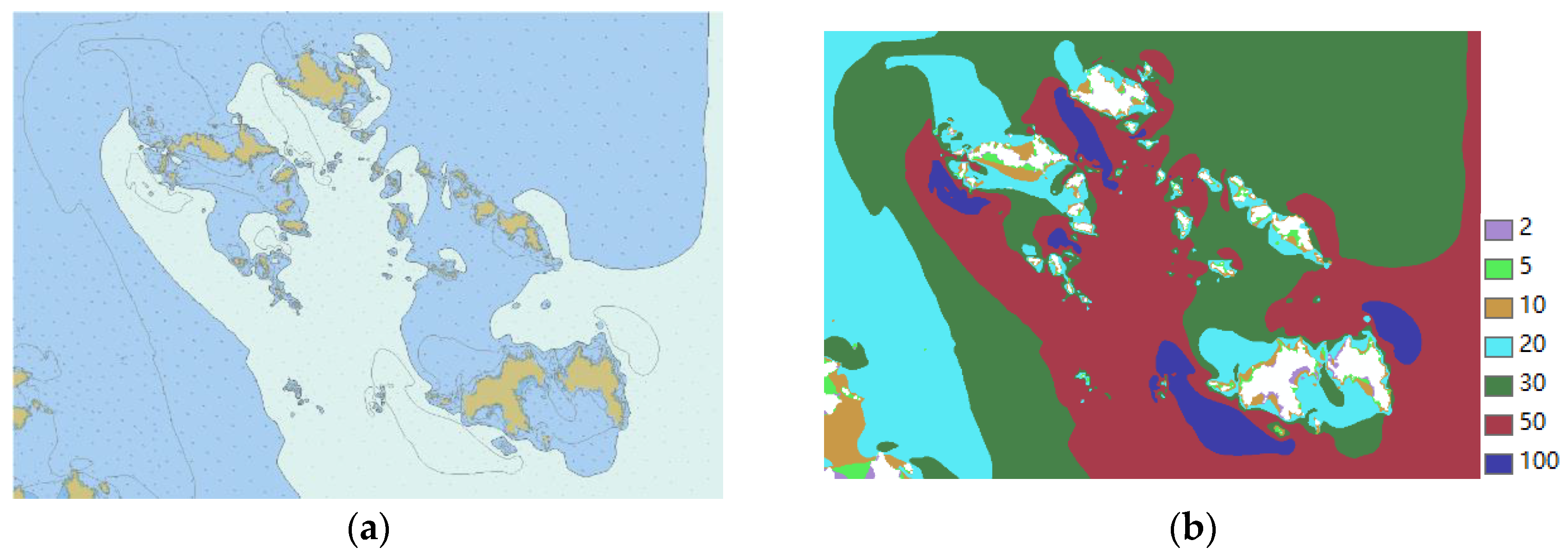
The spline function interpolation method with obstacles is performed to get the raster depth area with the water depth point selected as input point feature and the smoothing coefficient chosen as 0 and the grid size set as 25 m. The feasible space is updated according to the calculated minimum depth of safe navigation (1.29 m). Related parameters are shown in Table 6. The simulation is also based on the following assumptions: Assuming the unmanned vehicle as a mass point, unmanned vehicles can safely cross the junction vertex of the blocked grid and free gird between the obstacle area and the non-obstacle area, and unmanned vehicles can complete the turnaround operation in the grid. The proposed approach is simulated using Matlab R2018b. All simulations are performed on a PC with Microsoft Windows 10 as OS with Intel i5 2.712 GHz quad core CPU and 8 GB RAM.
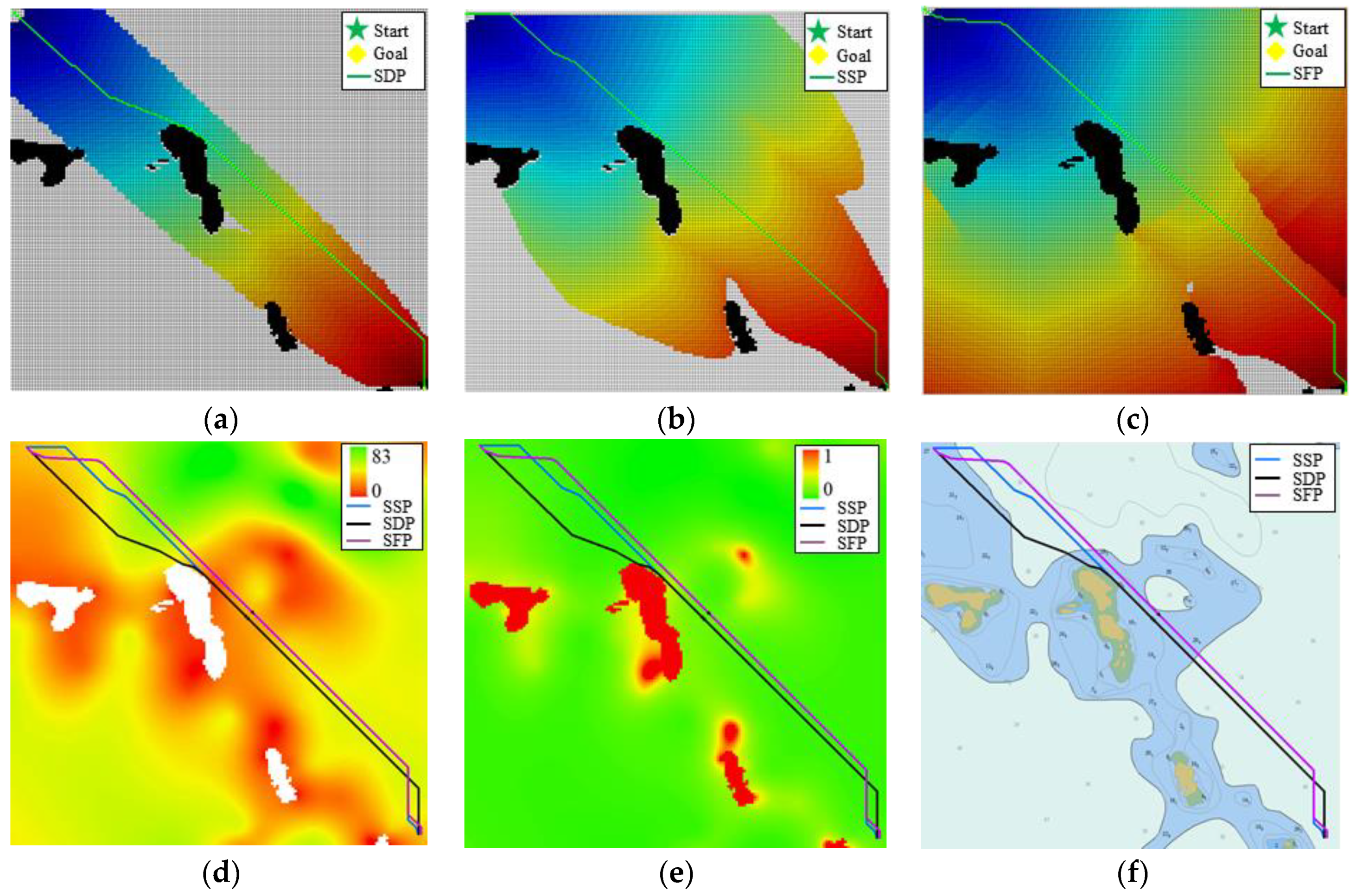
The positions of USV are represented by the grid index value of row and column where the point is located. S(500, 500) is chosen as the starting node and G(650, 650) as the goal node. Three kinds of cost function, including only distance, cost seeing Equation (15), only risk level cost seeing Equation (13), cost of combining seeing equation (16), were used to calculate the paths of shortest distance path (SDP), the shorter and safer path (SSP), the safest path (SFP) The results are shown in Figure 12. Compared with Figure 12a–c, it can be seen that the path planning algorithm considering water depth risk level will lead to more expanded nodes, so the search speed will be slower than A* and the expanded nodes of WDRLA* is less than those of SFP seeing Figure 12b,c. Figure 12d,e indicate that there is little difference between SSP and SFP, which means approximate depth risk level, but SDP is closer to the obstacle, so the risk level is much higher. Water depth risk level A* algorithm (WDRLA*) can reduce the depth risk and improve the safety of path, but sacrificing a certain calculation time.
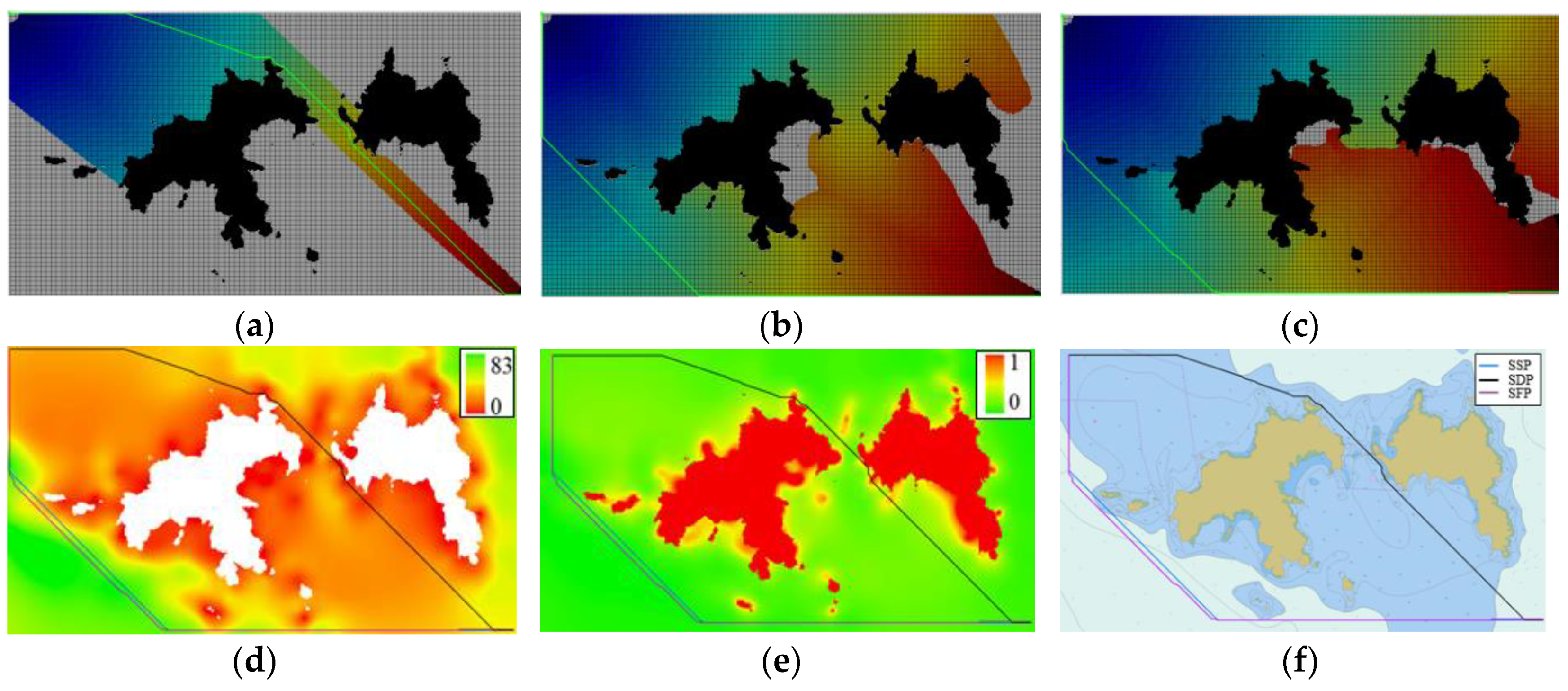
Take S(710, 902) as the starting node, and G(990, 1408) as the goal node, Results of three kinds of paths are shown in Figure 13. From Figure 13, it can be drawn that there are marked differences between SDP and SSP in shallow coastal waters. SDP passes through a narrow channel with shallow water depth which is more dangerous, while SSP and SFP avoid narrow channel by choosing deeper water area, where SSP reduces the risk of the path by 39.61% (see Table 7). At the same time, the number of extended nodes increases greatly, so WDLRA* path search process is slower than A*. SSP increases 1652m and 10.54% in length compared with SDP. The length of SSP and SFP is approximate, but SSP with less expanded nodes.
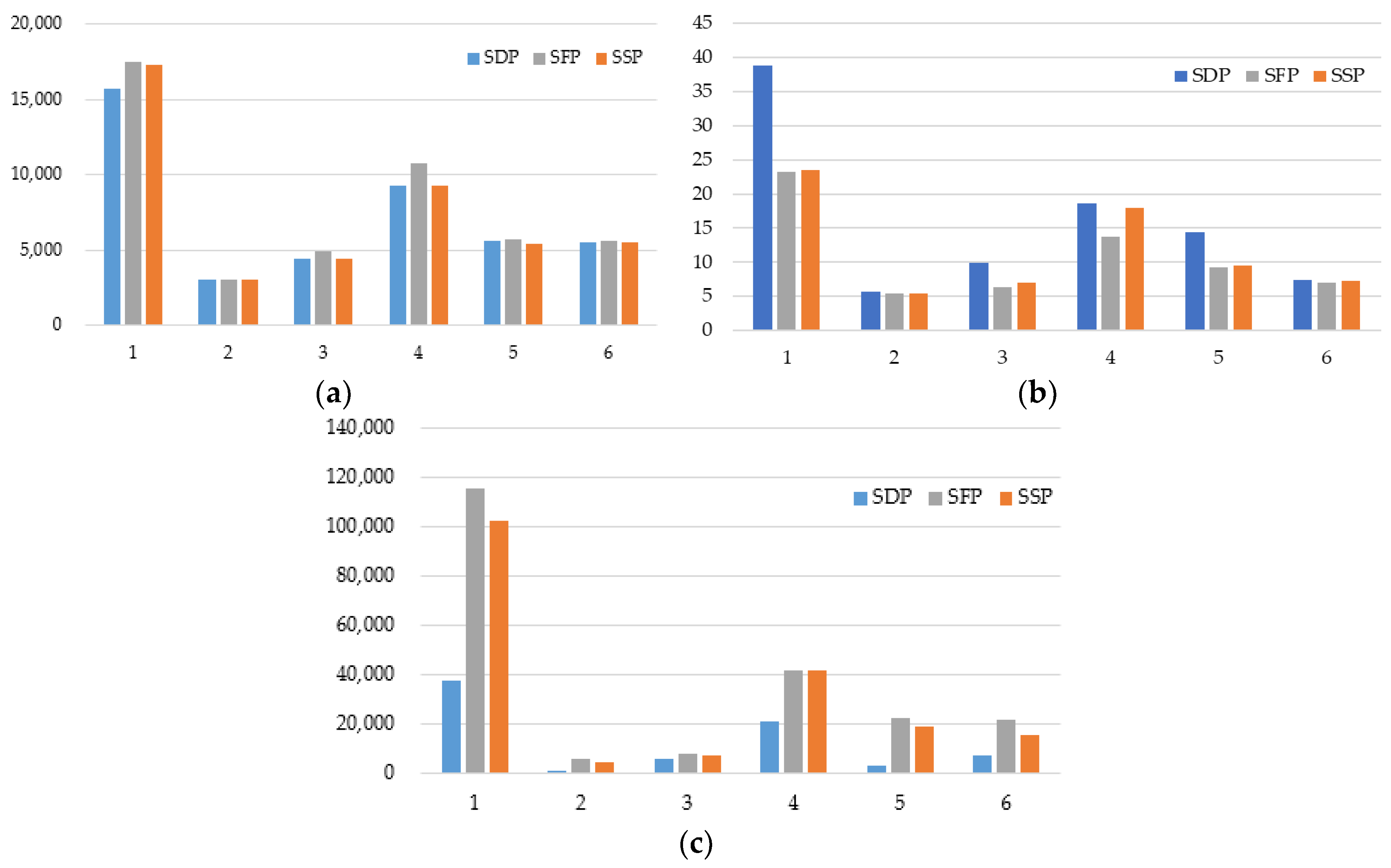
In order to determine the reliability and consistency of the algorithm furtherly, disparate starting nodes and end nodes cases are simulated, and several parameters, such as the path length, the number of expanded nodes, and the risk level of the path, are compared simultaneously, in which the depth risk level is calculated by Equations (11)–(13). All of the results are shown in Table 7. From Table 7 combined with Figure 12, Figure 13 and Figure 14, it can be seen that the depth risk level of the path can be reduced, and the path is relatively short, especially in the area with complicated underwater topography, such as Figure 13 with WDLRA* algorithm, but in the cost of decreasing computational efficiency with redundant expanded nodes (see Figure 12c and Figure 13c). This method can ensure the safety of small USV navigating in complicated sea areas.

5. Conclusions

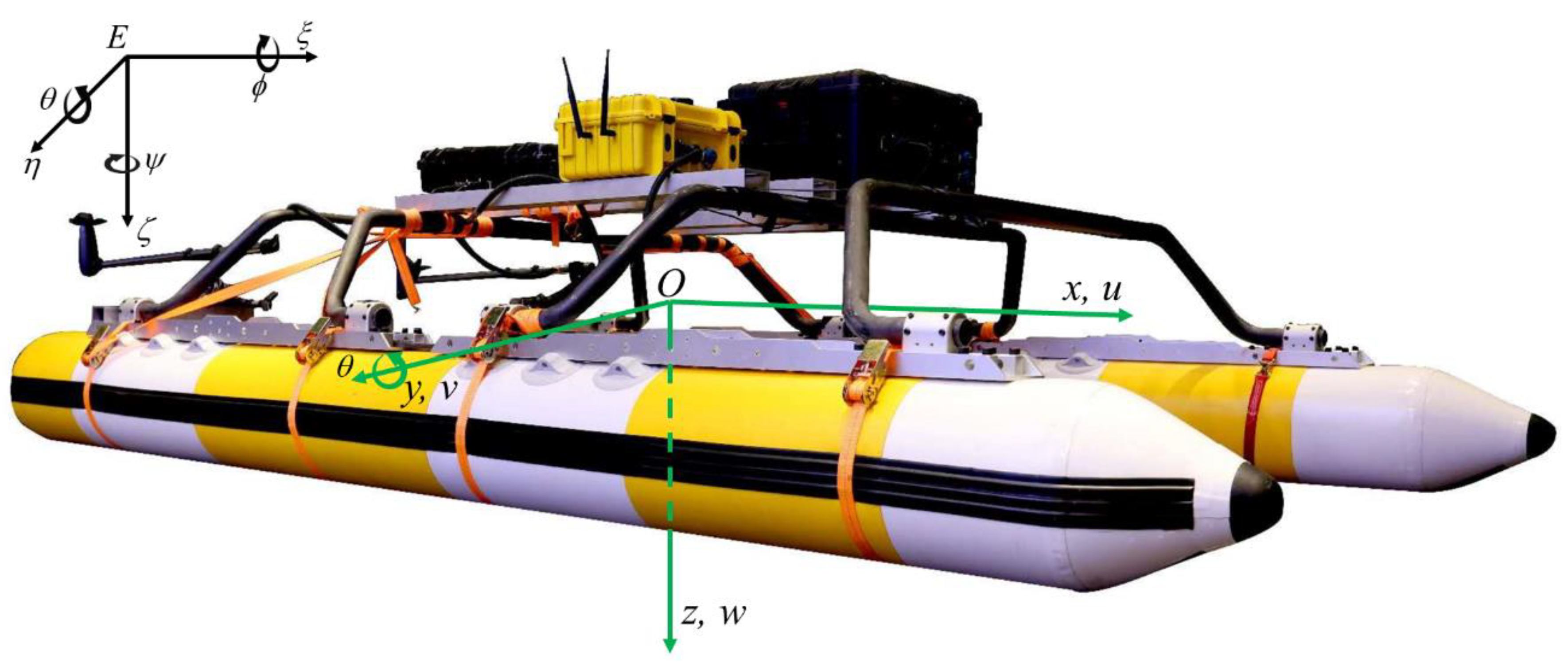
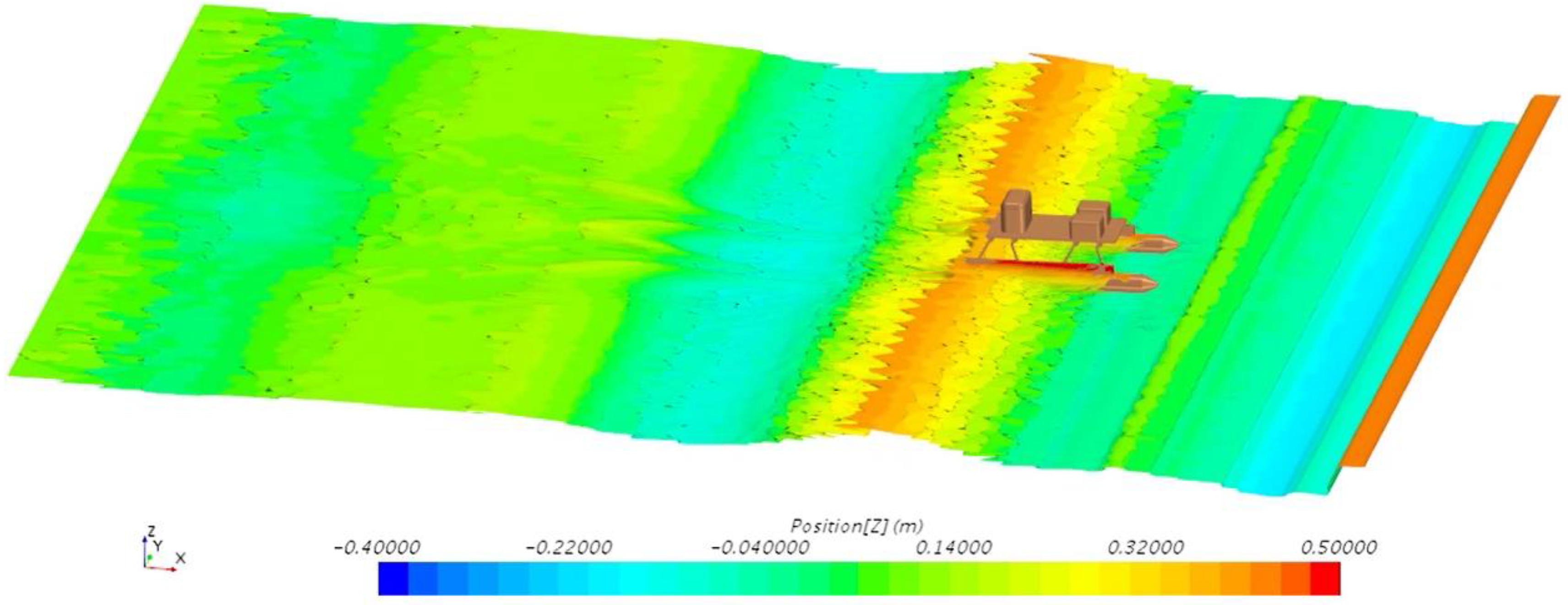
In this paper, hydrodynamic numerical simulation of a new marine surveying and mapping USV platform developed by the author’s research group is performed to evaluate its navigation status in irregular waves. It is found that the heave and pitch of the USV decrease with the increase of velocity and increase with the increase of significant wave height. The heave and pitch navigation status of the unmanned surface vehicle is evaluated through the analysis of 9 working conditions to ascertain minimum safe depth for navigation.
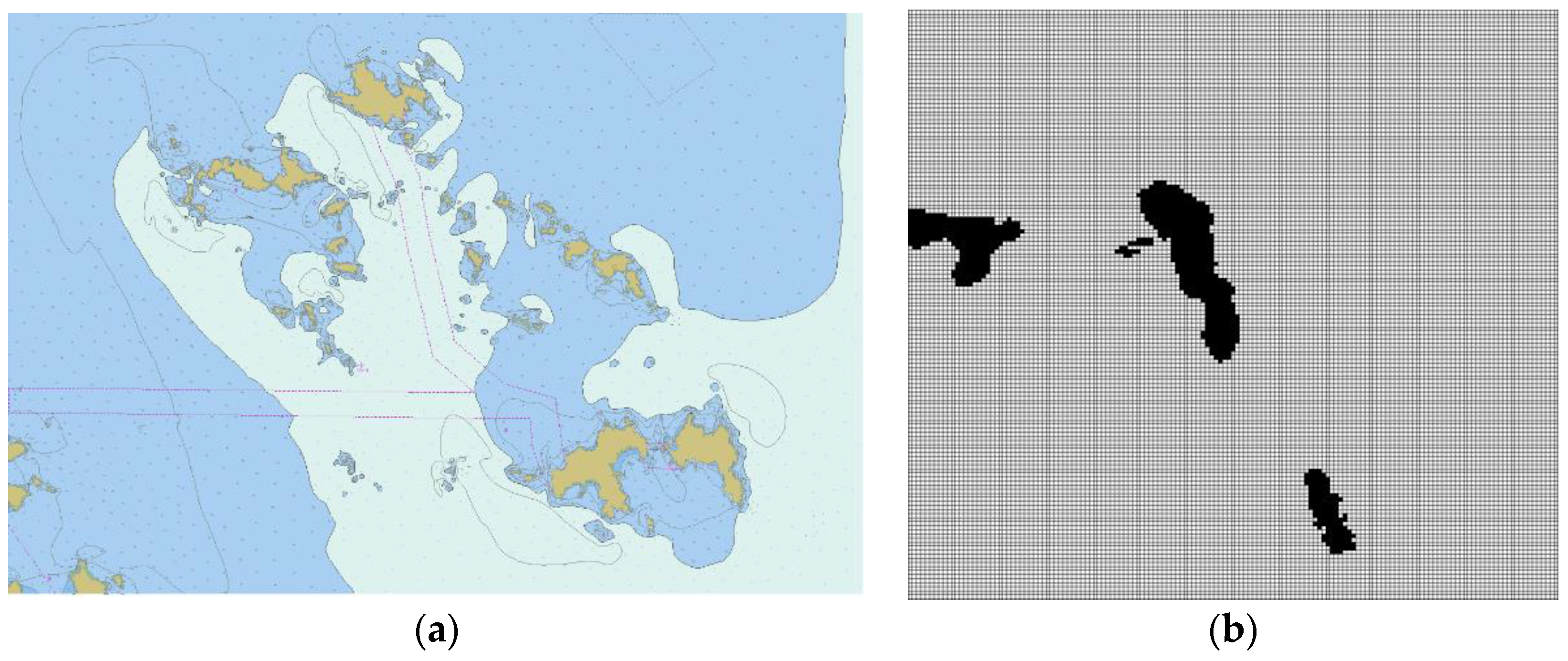
A grid environment modeling method considering water depth is carried out, in which the spline function interpolation algorithm with obstacles is employed to acquire the gridding prediction depth according to the discrete sparse depth points of ENC. The grid modeling method considering water depth can make the utmost of the water depth information provided by ENC to evaluate the depth risk level of path of unmanned surface vehicles.
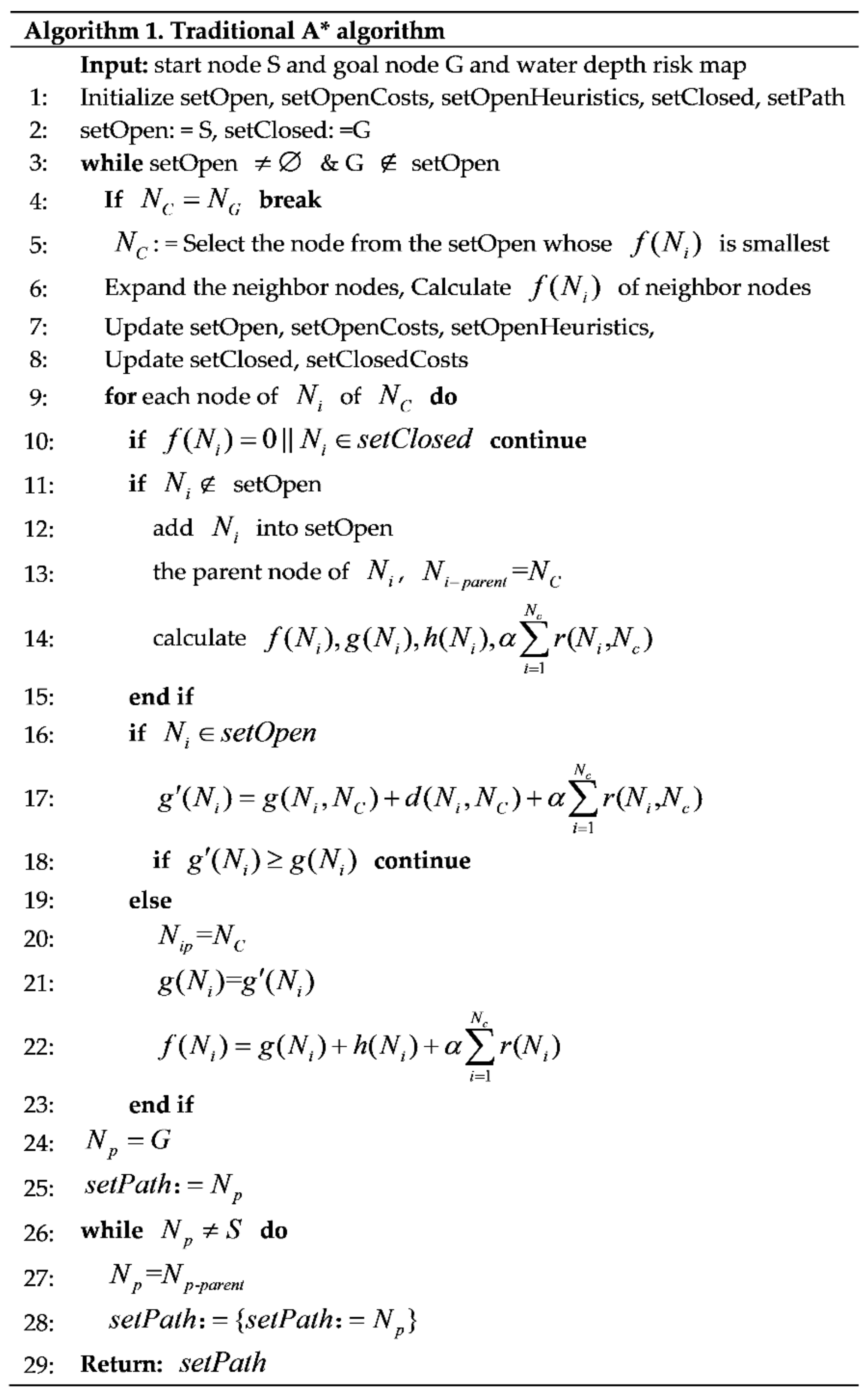
The quantitative evaluation method of the depth risk level of the path is proposed, and the simulation of path planning is carried out based on A* algorithm using depth hazard degree as an index, named the water depth risk level A* algorithm (WDRLA*). The results show that WDRLA* can hit a safer and shorter path taking into account of the mean draft, the hydrodynamic property, including the maximum heave value and the maximum pitch angle of a USV sailing in an irregular wave, position errors, including ENC positioning errors, positioning system errors and chart depth errors. WDRLA* algorithm can reduce the risk of planned paths in shallow offshore waters to ensure the navigation safety of a USV. The method of path depth risk assessment is not only appropriate to USV path planning, but also can provide guidance for manned ship path planning.
The works are still not completed for the limitations existing. For example, we neglected the influence of tide to water depth, which determines dynamic depth, since the depth on ENC is defined as the vertical distance between the theoretically lowest tide level and seabed. In the future, dynamic water depth will be involved in to acquire bathymetric in better accuracy. The search efficiency of the safe path planning algorithm is expected to be improved in the future.

Supplementary Materials

The following are available online at https://www.mdpi.com/2076-3417/9/16/3228/s1, Figure S1: Heave versus time, Figure S2: Pitch versus time.

Author Contributions

The manuscript was written S.L. and C.W. All authors discussed the original idea. conceptualization, S.L.; methodology, S.L. and C.W.; software, S.L.; validation, S.L.; formal analysis, C.W.; investigation, S.L.; resources, A.Z.; data curation, A.Z.; writing—original draft preparation, S.L. and C.W.; writing—review and editing, A.Z. and C.W.; visualization, S.L. and C.W.; project administration, A.Z.; funding acquisition, A.Z. and C.W.

Funding

This research was funded by National key research and development program of China, grant number 2018YFC1407400.

Conflicts of Interest

The authors declare no conflict of interest.

References

  1. Liu, Z.X.; Zhang, Y.M.; Yu, X.; Yuan, C. Unmanned surface vehicles.: An overview of developments and challenges. Annu. Rev. Control 2016, 41, 71–93. [Google Scholar] [CrossRef]
  2. Zheng, H.; Negenborn, R.R.; Lodewijks, G. Survey of approaches for improving the intelligence of marine Surface Vehicles. In Proceedings of the 16th International IEEE Conference on Intelligent Transportation Systems (ITSC 2013), The Hague, The Netherlands, 6–9 October 2013; pp. 1217–1223. [Google Scholar]
  3. Mohanan, M.G.; Salgoankar, A. A survey of robotic motion planning in dynamic environments. Robot. Auton. Syst. 2018, 100, 171–185. [Google Scholar] [CrossRef]
  4. Macharet, D.G.; Campos, M.F.M. A survey on routing problems and robotic systems. Robotica 2018, 36, 1781–1803. [Google Scholar] [CrossRef]
  5. Campbell, S.; Naeem, W.; Irwin, G.W. A review on improving the autonomy of unmanned surface vehicles through intelligent collision avoidance manoeuvres. Annu. Rev. Control 2012, 36, 267–283. [Google Scholar] [CrossRef] [Green Version]
  6. Liu, Y.C.; Bucknall, R. Path planning algorithm for unmanned surface vehicle formations in a practical maritime environment. Ocean Eng. 2015, 97, 126–144. [Google Scholar] [CrossRef]
  7. Wu, P.P.; Campbell, D.; Merz, T. Multi-objective four-dimensional vehicle motion planning in large dynamic environments. IEEE Trans. Syst. Man Cybern. B Cybern. 2011, 41, 621–634. [Google Scholar] [CrossRef] [PubMed]
  8. Ma, Y.; Hu, M.Q.; Yan, X.P. Multi-objective path planning for unmanned surface vehicle with currents effects. ISA Trans. 2018, 75, 137–156. [Google Scholar] [CrossRef] [PubMed]
  9. Hart, P.E.; Nilsson, N.J.; Raphael, B. A formal basis for the heuristic determination of minimum cost paths. IEEE Trans. Syst. Sci. Cybern. 1968, 4, 100–107. [Google Scholar] [CrossRef]
  10. Song, R.; Liu, Y.; Bucknall, R. Smoothed A* algorithm for practical unmanned surface vehicle path planning. Appl. Ocean Res. 2019, 83, 9–20. [Google Scholar] [CrossRef]
  11. Nash, A.; Koenig, S. Any-Angle Path Planning. AI Mag. 2013, 34, 85–107. [Google Scholar] [CrossRef] [Green Version]
  12. Choi, S.; Yu, W. Any-angle path planning on non-uniform costmaps. In Proceedings of the 2011 IEEE International Conference on Robotics and Automation ICRA, Shanghai, China, 9–13 May 2011; pp. 5615–5621. [Google Scholar]
  13. Kim, H.; Lee, T.; Chung, H.; Son, N.; Myung, H. Any-angle Path Planning with Limit-Cycle Circle Set for Marine Surface Vehicle. In Proceedings of the 2012 IEEE International Conference on Robotics and Automation ICRA, Saint Paul, MN, USA, 14–18 May 2012; pp. 2275–2280. [Google Scholar]
  14. Nash, A.; Koenig, S.; Likhachev, M. Incremental Phi*: Incremental Any-Angle Path Planning on Grids. In Proceedings of the International Joint Conference on Artificial Intelligence (IJCAI), Pasadena, CA, USA, 11–17 July 2009; pp. 1824–1830. [Google Scholar]
  15. Nash, A.; Koenig, S.; Tovey, C. Lazy Theta*: Any-Angle Path Planning and Path Length Analysis in 3D. In Proceedings of the Third Annual Symposium on Combinatorial Search, SOCS 2010, Stone Mountain, Atlanta, GA, USA, 8–10 July 2010; pp. 147–154. [Google Scholar]
  16. Daniel, K.; Nash, A.; Koenig, S.; Felner, A. Theta*: Any-Angle Path Planning on Grids. J. Artif. Intell. Res. 2010, 39, 533–579. [Google Scholar] [CrossRef] [Green Version]
  17. Yang, J.M.; Tseng, C.M.; Tseng, P.S. Path planning on satellite images for unmanned surface vehicles. Int. J. Nav. Arch. Ocean 2015, 7, 87–99. [Google Scholar] [CrossRef] [Green Version]
  18. Liu, C.G.; Mao, Q.Z.; Chu, X.M.; Xie, S. An Improved A-Star Algorithm Considering Water Current, Traffic Separation and Berthing for Vessel Path Planning. Appl. Sci. 2019, 9, 1057. [Google Scholar] [CrossRef]
  19. Singh, Y.; Sharma, S.; Sutton, R.; Hatton, D.; Khan, A. A constrained A* approach towards optimal path planning for an unmanned surface vehicle in a maritime environment containing dynamic obstacles and ocean currents. Ocean Eng. 2018, 169, 187–201. [Google Scholar] [CrossRef] [Green Version]
  20. Larson, J.; Bruch, M.; Ebken, J. Autonomous navigation and obstacle avoidance for unmanned surface vehicles. Proc. SPIE 2006, 6230. [Google Scholar] [CrossRef]
  21. Svec, P.; Schwartz, M.; Thakur, A.; Gupta, S.K. Trajectory Planning with Look-Ahead for Unmanned Sea Surface Vehicles to Handle Environmental Disturbances. In Proceedings of the 2011 IEEE/RSJ International Conference on Intelligent Robots and Systems, San Francisco, CA, USA, 25–30 September 2011; pp. 1154–1159. [Google Scholar]
  22. Naeem, W.; Irwin, G.W.; Yang, A.L. COLREGs-based collision avoidance strategies for unmanned surface vehicles. Mechatronics 2012, 22, 669–678. [Google Scholar] [CrossRef]
  23. Svec, P.; Gupta, S.K. Automated synthesis of action selection policies for unmanned vehicles operating in adverse environments. Auton. Robot. 2012, 32, 149–164. [Google Scholar] [CrossRef]
  24. Soulignac, M. Feasible and Optimal Path Planning in Strong Current Fields. IEEE Trans. Robot. 2011, 27, 89–98. [Google Scholar] [CrossRef]
  25. Naus, K.; Wąż, M. The idea of using the A* algorithm for route planning an unmanned vehicle “Edredon”. Zesz. Nauk. Akad. Morska W Szczec. 2013, 36, 143–147. [Google Scholar]
  26. Kim, H.; Park, B.; Myung, H. Curvature Path Planning with High Resolution Graph for Unmanned Surface Vehicle. In Robot Intelligence Technology and Applications 2012; Springer: Berlin/Heidelberg, Germany, 2013; pp. 147–154. [Google Scholar]
  27. Lee, T.; Kim, H.; Chung, H.; Bang, Y.; Myung, H. Energy efficient path planning for a marine surface vehicle considering heading angle. Ocean Eng. 2015, 107, 118–131. [Google Scholar] [CrossRef]
  28. Fossen, T.I. Handbook of Marine Craft Hydrodynamics and Motion Controli, 1st ed.; John Wiley & Sons Ltd.: Chichester, UK, 2011. [Google Scholar]
  29. Dhanak, M.R.; Xiros, N.I. Springer Handbook of Ocean Engineering; Springer: Berlin/Heidelberg, Germany, 2016. [Google Scholar]
  30. Kim, H.; Kim, D.; Shin, J.U.; Kim, H.; Myung, H. Angular rate-constrained path planning algorithm for unmanned surface vehicles. Ocean Eng. 2014, 84, 37–44. [Google Scholar] [CrossRef]
Figure 1. Multi-functional Marine mapping unmanned surface vehicles.
Applsci 09 03228 g001
Figure 2. Computational Domain.
Applsci 09 03228 g002
Figure 3. Mesh Generation and Distribution. (a) Three-dimensional Mesh Generation; (b) Grid Distribution Around the Wall.
Applsci 09 03228 g003
Figure 4. S57 Environmental Modeling Map (a) Study Area of S57 Electronic Chart. (b) Regional Grid Marine Environment Map with a resolution of 25 m × 25 m. In the picture, the white meshes represent the feasible region, while the black meshes are a barrier.
Applsci 09 03228 g004
Figure 5. Electronic navigation Chart and Grid Depth Distribution Map. (a) S57 Vector Electronic navigation Chart displayed by S52 Standard in the study area; (b) Isobath Area Map; (c) Depth Distribution Map obtained by spline function interpolation approach with obstacles, in which the blank area is an obstacle; (d) Overlay with discrete depth points, contours, islands and reefs and other obstacles. In the depth distribution map, the magenta area is an obstacle.
Applsci 09 03228 g005aApplsci 09 03228 g005b
Figure 6. Numerical simulation results of the unmanned vehicle.
Applsci 09 03228 g006
Figure 7. Analysis of heave of the USV.
Applsci 09 03228 g007
Figure 8. Maximum pitch Angle of nine cases.
Applsci 09 03228 g008
Figure 9. The depth hazard distribution map.
Applsci 09 03228 g009
Figure 10. A* path planning algorithm schematic diagram. (a) Schematic of adjacent node expansion; (b) The shortest path of A* algorithm. The green star represents the starting point, and the yellow diamond represents the goal point. The shortest path is the black line between the starting point and the end point. The color grids are expanded nodes. The deeper the blue is, the closer the starting point is, and the deeper the red is, the closer the end point is. A set of white grids represents a feasible space, and black grids are obstacles.
Applsci 09 03228 g010
Figure 11. WDRLA* algorithm pseudo code chart.
Applsci 09 03228 g011
Figure 12. Comparison of three kinds path. (a) Shortest distance path (SDP) that ignores the depth risk; (b) Shorter and safer path (SSP) that considers the depth risk level and distance. (c) Safest path (SFP) that considers only the depth risk. The colorful grids in figure (ac) are extended nodes. The space of white grids represents the feasible space, and the black grids are obstacles. (d) Three paths, shown on the depth distribution map. (e) Three paths, shown on the depth risk level distribution map. (f) Three paths, shown on S57 ENC. The black line is the SDP, the blue one is SSP, and the purple one is SFP.
Applsci 09 03228 g012
Figure 13. Comparison of three kinds path. (a) SDP that ignores the depth risk; (b) SSP that considers the depth risk level and distance. (c) SFP that considers only the depth risk. The colorful grids in figure (ac) are extended nodes. The space of white grids represents the feasible space, and the black grids are obstacles. (d) Three paths, shown on the depth distribution map. (e) Three paths, shown on the depth risk level distribution map. (f) Three paths, shown on S57 ENC. The black line is the SDP, the blue one is SSP, and the purple one is SFP.
Applsci 09 03228 g013
Figure 14. The comparation of key parameters of three different sorts of paths. (a) The total distance of the path. The unit of distance is m. (b) Water depth risk level of the path. (c) The number of expanded nodes of three sorts of cost functions.
Applsci 09 03228 g014
Table 1. Table of the unmanned surface vehicle parameters.
ParametersValue
Length3.2 m
Molded breadth2.2 m
Displacement92 kg (full load 140 kg)
Location of gravity center(1.285, 0.000, 0.600)
Moment of inertia of Y axis400 kg/ m 2
Draft0.5 m
Table 2. Cases list.
Case NumberSpeed (kn)Wave Height (m) F r   1
150.50.42
251.00.42
351.50.42
480.50.63
581.00.63
681.50.63
7110.50.84
8111.00.84
9111.50.84
1 F r : Volume Froude number, a non-dimensional parameter which presents the shape and the displacement of the ship.
Table 3. Numerical simulation methods.
Discretization MethodFinite Volume Method
SchemeSIMPLE
SolverImplicit Unsteady
GradientGreen-Guass Cell Based
PressureSecond Order
MomentumSecond Order Upwind
Transient FormulationSecond Order Implicit
Mesh motionOverset motion
Table 4. Mesh independency study.
MeshMesh 1Mesh 2Mesh 3
Number of meshs774,9211,373,4951,925,630
E = | 1 C ¯ d i / C ¯ d 3 | 1.13 × 10 3 4.35 × 10 3 --
Table 5. Interval table of electronic navigation chart (ENC) with different scales.
Plotting ScaleDepth Contour Interval
≥1:150,0000/2/5/10/20/30/50/100/200/500
≥1:1,000,000 and ≤1:150,0000/5/10/20/30/50/100/200/500/1000
≤1:1,000,0000/10/50/200/500/1000/2000/4000/6000
Table 6. Table of Related parameters.
ParametersValue
Cell size25 m × 25 m
L3.2 m
T ¯ 0.5 m
z max 0.3 m
θ max 11 °
e e n c 0.2 m
α 10
Table 7. Comparison of different starting and goal points.
TestStart PointGoal PointTotal Distance (m)Risk LevelNodes of Expanded
A*WDLRA*A*WDLRA*A*WDLRA*
1(710, 902)(990, 1408)15,667.517,319.538.8614223.4683037,682102,283
2(343, 975)(417, 1066)30633063.05.687365.4793613634469
3(408, 560)(520, 680)4457.754472.59.954727.0376958517679
4(200, 250)(410, 530)9270.59255.7518.6802917.9221121,40741,840
5(500, 889)(650, 1039)5641.55405.514.437469.53375297119,301
6(500, 500)(650, 650)5567.755567.757.396057.31804776115,533

