Article

Color–Texture Pattern Classification Using Global–Local Feature Extraction, an SVM Classifier, with Bagging Ensemble Post-Processing

by
Carlos F. Navarro
and
Claudio A. Perez
*
Image Processing Laboratory, Electrical Engineering Department and Advanced Mining Technology Center, Universidad de Chile, Santiago 8370451, Chile
*
Author to whom correspondence should be addressed.
Appl. Sci. 2019, 9(15), 3130; https://doi.org/10.3390/app9153130
Submission received: 12 June 2019 / Revised: 29 July 2019 / Accepted: 30 July 2019 / Published: 1 August 2019
(This article belongs to the Special Issue Texture and Colour in Image Analysis)

Abstract

:

Featured Application

The proposed method is a new tool to characterize colored textures and may be applied in various applications such as content image retrieval, characterization of rock samples, biometrics, classification of fabrics, and in non-destructive inspection in wood, steel, ceramic, fruit, and aircraft surfaces.

Abstract

Many applications in image analysis require the accurate classification of complex patterns including both color and texture, e.g., in content image retrieval, biometrics, and the inspection of fabrics, wood, steel, ceramics, and fruits, among others. A new method for pattern classification using both color and texture information is proposed in this paper. The proposed method includes the following steps: division of each image into global and local samples, texture and color feature extraction from samples using a Haralick statistics and binary quaternion-moment-preserving method, a classification stage using support vector machine, and a final stage of post-processing employing a bagging ensemble. One of the main contributions of this method is the image partition, allowing image representation into global and local features. This partition captures most of the information present in the image for colored texture classification allowing improved results. The proposed method was tested on four databases extensively used in color–texture classification: the Brodatz, VisTex, Outex, and KTH-TIPS2b databases, yielding correct classification rates of 97.63%, 97.13%, 90.78%, and 92.90%, respectively. The use of the post-processing stage improved those results to 99.88%, 100%, 98.97%, and 95.75%, respectively. We compared our results to the best previously published results on the same databases finding significant improvements in all cases.

1. Introduction

Texture pattern classification was considered an important problem in computer vision for many years because of the great variety of possible applications, including non-destructive inspection of abnormalities on wood, steel, ceramics, fruit, and aircraft surfaces [1,2,3,4,5,6]. Texture discrimination remains a challenge since the texture of objects varies significantly according to the viewing angle, illumination conditions, scale change, and rotation [1,4,7,8]. There is also the special problem of color image retrieval related to appearance-based object recognition, which is a major field of development for several industrial vision applications [1,4,7,8].
Feature extraction of color, texture, and shape from images was used successfully to classify patterns by reducing the dimensionality and the computational complexity of the problem [3,9,10,11,12,13,14,15,16]. Determining the appropriate features for each problem is a recurring challenge which is yet to be fully met by the computer vision community [1,3,16]. Feature extraction and selection enable representation of the information present in the image, and limit the number of features, thus allowing further analysis within a reasonable time. Feature extraction was used in a wide range of applications, such as biometrics [12,14,15], classification of cloth, surfaces, landscapes, wood, and rock minerals [16,17], saliency detection [18], and background subtraction [19], among others. During the past 40 years, while a substantial number of methods for grayscale texture classification were developed [3,5], there was also a growing interest in colored textures [1,2,9,10,13,20,21]. The adaptive integration of color and texture attributes into the development of complex image descriptors is an area of intensive research in computer vision [21]. Most of these investigations focused on the integration process in applications for digital image segmentation [20,22] or the aggregation of multiple preexisting image descriptors [23]. Deep learning was applied successfully to object or scene recognition [24] and scene classification [25], and the use of deep neural networks for the classification of image datasets where texture features are important for generating class-conditional discriminative representations was investigated [26].
Current approaches to color texture analysis can be classified into three groups: the parallel approach, the sequential approach, and the integrative approach [11,27]. The parallel approach considers texture and color as separate phenomena. Color analysis is based on the color distribution in an image, without regard to the spatial relationship between the intensities of the pixels. Texture analysis is based on the relative variation of the intensity of the neighbors, regardless of the color of the pixels. In Reference [2], the authors first converted the original RGB images into other color spaces: HSI (Hue, Saturation, Lightness), CIE XYZ (Comission Internationale de l´Éclairage Tristimulus values), YIQ (Luminance In phase Quadrature), and CIELAB (Comission Internationale de l´Éclairage Lightness-Green-Blue), and then extracted the texture features and color separately. In a similar manner, as reported in Reference [13], the images were transformed to the color spaces HSV and YCbCr, obtaining wavelet intensity channel features of first-order statistics on each channel. The choice of the best performing color space was an open question in recent years, since using one space instead of another can bring considerable improvements in certain applications [28]. The quaternion representation of color was shown to be effective in segmentation in Reference [29] and the feature extraction method, binary quaternion moment preserving (BQMP), is a method of image binarization using quaternions, with the potential for being a powerful tool in color image analysis [6].
In the sequential approach to color texture analysis, the first step is to apply a method of indexing color images. As a result, indexed images are processed obtaining grayscale textures. The co-occurrence matrix was used extensively since it represents the probability of occurrence of the same color pixel pair at a given distance [9]. Another example of this approach is based on texture descriptors using three different color indexing methods and three different texture features [11]. This results in nine independent classifiers that are combined through various schemes.
Integration models are based on the interdependence of texture and color. These models can be divided into single bands, if the data of each channel is considered separately, or a multiband, if two or more channels are considered together. The advantage of the single-band approach is the easy adaptation of classical models based on a grayscale domain, such as Gabor filters [15,30,31,32], local binary patterns (LBP) or variants [5,7,8,33,34,35,36,37,38], Galois fields [39], or Haralick statistics [3]. In Reference [2], the main objective was to determine the contribution of color information for the overall performance of classification using Gabor filters and co-occurrence measures, yielding results almost 10% better than those obtained with only grayscale images. In Reference [4], the results reported using co-occurrence matrices reached 94.41% and 99.07% on the Outex and Vistex databases, respectively. Different classifiers, such as k-nearest neighbors, neural networks, and support vector machines (SVM) [40], are used to combine features. The latter was proven to be more efficient when feature selection is performed [41,42] or clustering is used [22].
There are other methods that reached the best results in color texture analysis on databases that are publicly available. In Reference [1], a multi-scale architecture (Multi-Scale Supervised self-Organizing Orientational-invariant Neural or multi-scale SOON) was presented that reached 91.03% accuracy on the Brodatz database, which contains 111 different colored textures. These results were compared with those of two previous studies on the same database, reported in References [43,44], which reached classification rates of 89.71% and 88.15%, respectively. Another approach used all the information from sensors that created the image [4]. This method improved the results to 98.61% and 99.07%, on the same database, but required a non-trivial change in the architecture of the data collection. A texture descriptor based on a local pattern encoding scheme using local maximum sum and difference histograms was proposed in Reference [8]. The experimental results were tested on the Outex and KTH-TIPS2b databases reaching 95.8% and 91.3%, respectively. In References [32,33,36,39], the methods were not tested in the complete databases. In References [26,45,46], the methods used a different metric to calculate the classification.
A new method for the classification of complex colored textures is proposed in this paper. The images are divided into global and local samples where features are extracted to provide a new representation into global and local features. The feature extraction from different samples of the image using quadrants is described. The extraction of the features in each of the image quadrants, obtaining color and texture features in different spatial scales, is presented: the global scales using the whole image, and the local scales using quadrants. This representation seems to capture most of the information present in the image to improve colored texture classification. Then, a support vector machine classification that was performed is reported and, finally, the post-processing stage using the bagging that was implemented is presented. The proposed method was tested on four different databases: Colored Brodatz Texture [20], VisTex [4], Outex [47], and KTH-TIPS2b [48] databases. The subdivision of the training partition of the database into sub-images while extracting information from each sub-image of different sizes is also new. The results were compared to state-of-the art methods whose results were already published on the same databases.

2. Materials and Methods

The objective was to create a method for colored texture classification that would improve the classification of different complex color patterns. The BQMP method was used previously in color data compression, color edge detection, and multiclass clustering of color data, but not in classification [6,47]. The BQMP reduces an image to representative colors and creates a histogram that indicates the parts of the image that are represented by these colors. Therefore, the color features of the image are represented in this histogram. Haralick’s features [3] are often extracted to characterize textures that measure the grayscale distribution, as well as considering the spatial interactions between pixels [3,9,23,38]. Creating a training set is part of the strategy for obtaining local and global features that contain all the information, local and global, for achieving correct classification. Different classifiers, such as k-nearest neighbors, neural networks, and support vector machines (SVM) [41], are used to combine features. In Reference [44], an SVM showed good performance compared to 16 different classification methods.

2.1. Feature Extraction Quadrants

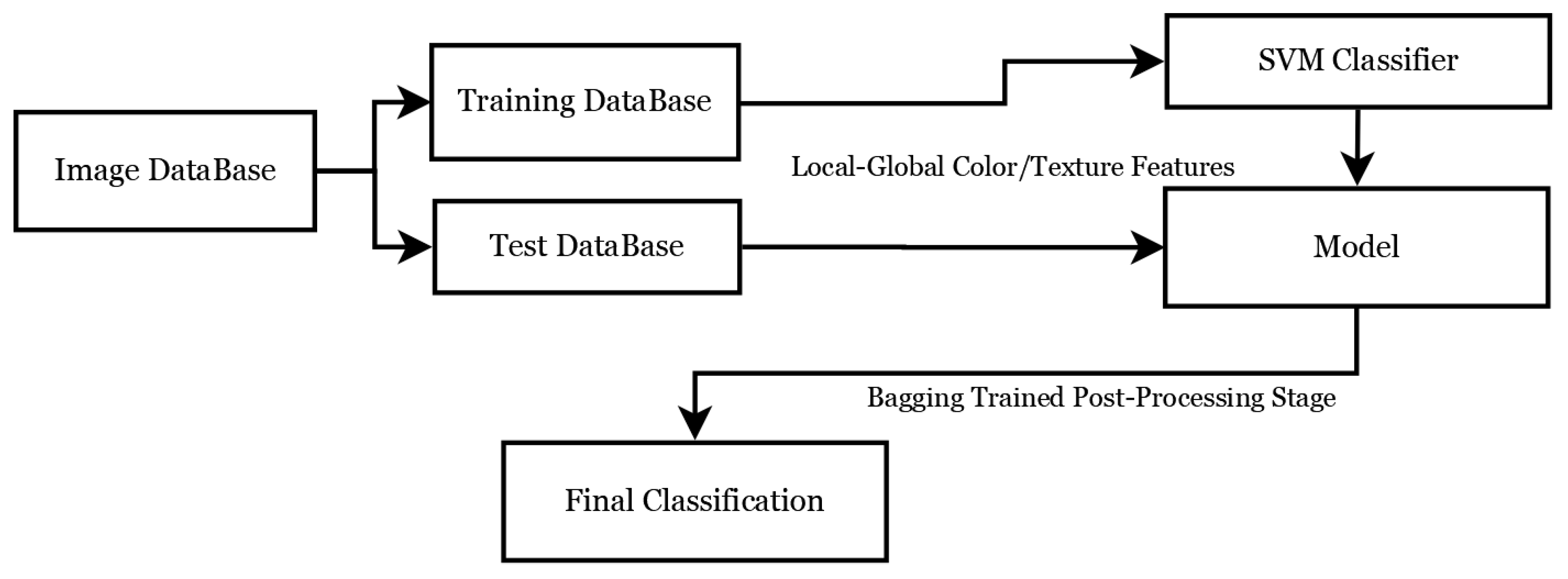
The proposed method divides the images to obtain local and global features from them. The method consists of four stages: firstly, the images in the database are divided into images to be used in training and those to be used in testing. In the second stage, color and texture features are extracted from the training images on both global and local scales. In the third stage, color and texture features are fused to become the inputs to the SVM classifier, and the last stage is a post-processing stage that uses bagging with the test images for classification. These stages are summarized in the block diagram of Figure 1.
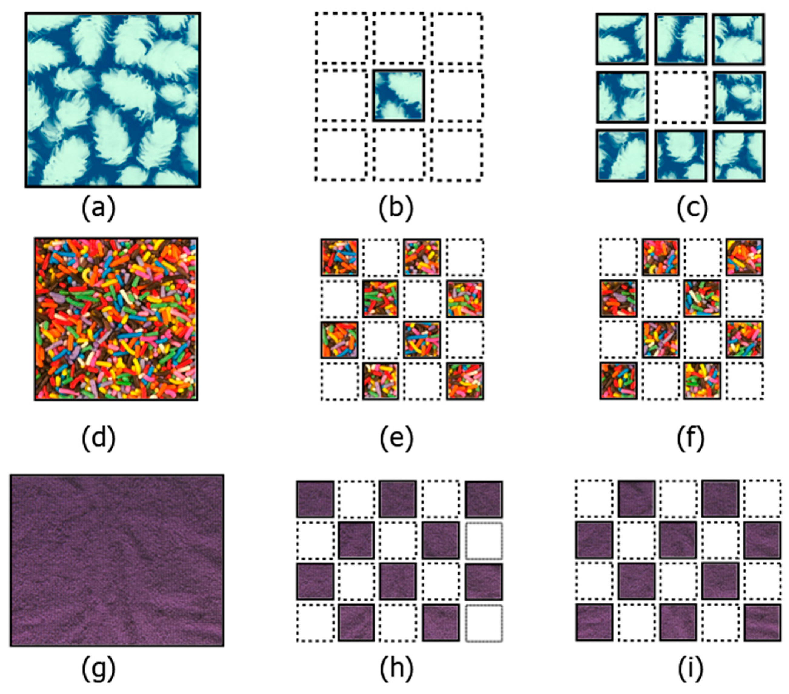
To be able to compare the performance of our method with previously published results, we used the same partition, into training and testing sets, in each database. In the case of the Brodatz database, as in Reference [1], each colored texture image was partitioned into nine sub-images, using eight for training, and one for testing. An example of this partition is shown in Figure 2a–c. The Brodatz Colored Texture (CBT) database has 111 images of 640 × 640 pixels. Each image in the database has a different texture.
For the Vistex database, the number of training and testing images was eight as in Reference [4]. In the case of the Outex database, the number of training and testing sub-images was 10 as in References [4,9,47]. The KTH-TIPS2b database was already partitioned into four samples, and we performed a cross-validation as in References [7,48].
In each case, we subdivided the training database and the test database using two parameters: n is the number of images divided by side, and r is the times we take n2 local images from each sample. We can take r × n2 local images to extract features from all the samples in each database. 
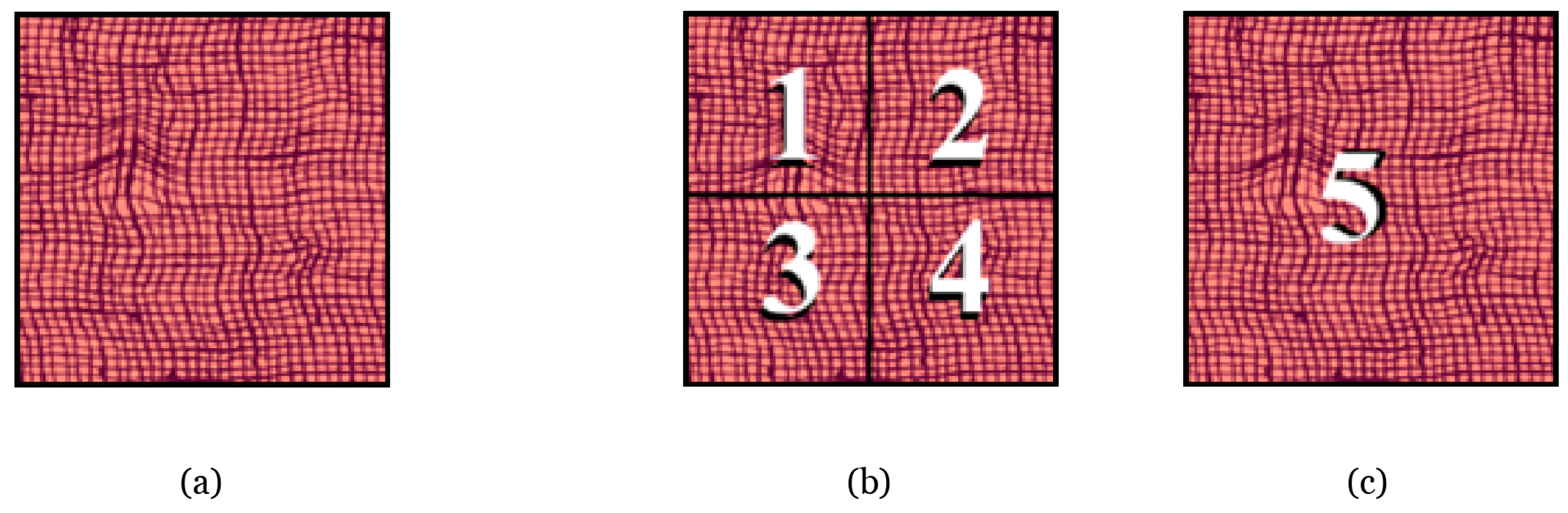
Figure 3 shows the image subdivision scheme for the training images. It can be observed that the partitioning scheme allows obtaining features from different parts of the image, at a global and local level. The method was designed to follow this approach so that no relevant information would be lost from the image.
BQMP and Haralick (without using co-occurrence matrices) are invariant to translation and rotation; the same features are obtained if an exchange of the position of two pixels is made in the image [3,6,47]. This suggests that there is spatial information present in the image that is not extracted by these features. In our proposed method, we use the two-scale scheme, local and global, to add spatial information to the extracted features. This is shown in Figure 4, and explained in detail in Section 2.4. The BQMP and Haralick features are extracted in each quadrant. The test images can be subdivided into local images from which the features are extracted. This allows the creation of a post-processing stage in which a bagging process can be performed. Our method is invariant to translation because of the randomness of the local image positions, but it is partially invariant to rotation because the features are concatenated in an established order. However, color features, as well as Haralick texture features, are invariant to rotation. There are problems where orientation dependency is desirable [49].

2.2. BQMP Color Feature Extraction

After image subdivision, the BQMP was applied to each one of the local and global sub-images. This method is used as a tool for extracting color features using quaternions. Each pixel in the RGB space is represented as a quaternion. In Reference [6], the authors showed that it is possible to obtain two quaternions that represent a different part of the image, obtaining a binarization of the image in the case of two colors. For more colors, this method can be performed recursively n times, yielding 2n representatives of an image, and the part of the image that each representative represents in a histogram. The process is repeated, obtaining a result with a binary tree structure. 
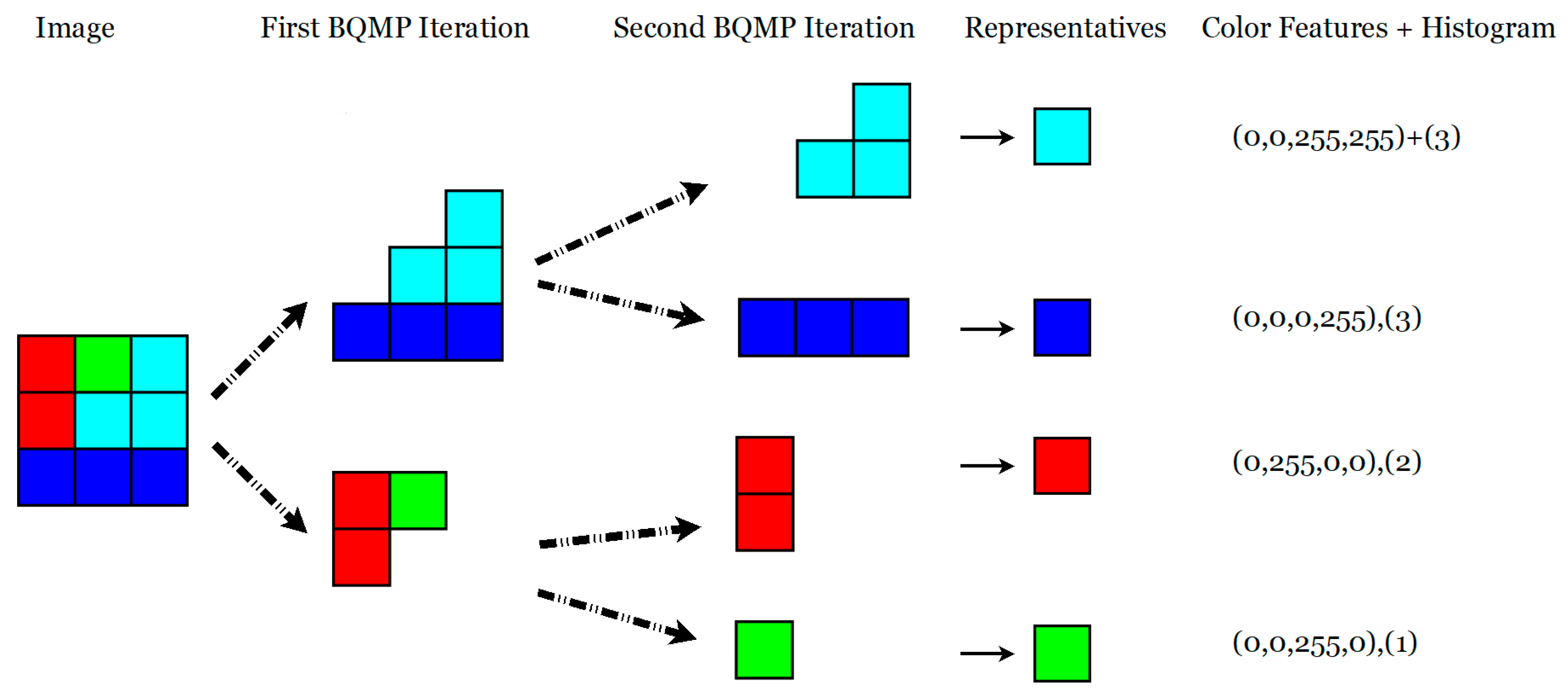
Figure 5 shows the BQMP method for the case of four different colors. The numbers show the color code and the number of pixels represented by each. Figure 6 shows the second iteration for the same case.
The feature vector is formed by concatenating the color code and histograms, through normalization. This vector is concatenated with the ones in other scales and the ones made using Haralick statistics, which are also normalized.

2.3. Haralick Texture Features

The Haralick texture features are angular second moment, contrast, correlation, sum of squares, inverse difference moment, sum average, sum variance, sum entropy, entropy, difference variance, difference entropy, and information measures of correlation [3]. Other measures characterize the complexity and nature of tone transitions in each channel of the image. The usual practice is to use the first 13 Haralick features with a co-occurrence matrix [4], but in this work, we extracted the 13Haralick features directly from the images because they provide spatial information from different regions within each image.
The Haralick features used to extract the texture features were Equations (1)–(13), and Equations (14)–(21) explain the notation employed.
Angular second moment:
f 1 = i j p ( i , j ) 2 .
Contrast:
f 2 = n = 0 N 1 n 2 i = 1 N j = 1 N p ( i , j ) ,
where | i j | = n .
Correlation:
f 3 = i j ( i j ) p ( i , j ) μ x μ y σ x σ y ,
where μ x , μ y , σ x , and σ y are the means and standard deviations of p x and p y .
Sum of squares:
f 4 = i j ( i μ ) 2 p ( i , j ) .
Inverse difference moment:
f 5 = i j p ( i , j ) 1 + ( i j ) 2 .
Sum average:
f 6 = i = 2 2 N i p x + y ( i ) .
Sum variance:
f 7 = i = 2 2 N ( i f 8 ) 2 p x + y ( i ) .
Sum entropy:
f 8 = i = 2 2 N p x + y ( i )   log ( p x + y ( i ) ) .
Entropy:
f 9 = i j p ( i , j )   log   ( p ( i , j ) ) .
Difference variance:
f 10 = V a r ( p x y ) .
Difference entropy:
f 11 = i = 0 N 1 p x y ( i )   log ( p x y ( i ) ) .
Information measures of correlation:
f 12 = f 9 H X Y 1 m a x ( H X , H Y ) ,
f 13 = 1 exp ( 2 ( H X Y 2 f 9 ) ) 1 2 ,
where HX and HY are the entropies of px and py, and
H X Y = i j p ( i , j )   log ( p ( i , j ) ) ,
H X Y 1 = i j p ( i , j )   log ( p x ( i ) p y ( j ) ) ,   a n d
H X Y 2 = i j p x ( i ) p y ( j )   log ( p x ( i ) p y ( j ) ) .  
In Equations (1)–(13), to calculate the features, the following notation was used:
p ( i , j ) ,
which is the (i,j)th pixel in a gray sub-image matrix.
p x ( i ) ,
which is the ith entry in the sub-image matrix, obtained by summing the rows of p.
p y ( j ) ,
which is the jth entry in the sub-image matrix, obtained by summing the columns of p.
P x + y ( k ) = i = 1 n j = 1 n p ( i , j ) ,
where i + j = k and k = 2, 3, …, 2N.
P x y ( k ) = i = 1 n j = 1 n p ( i , j ) ,
where |ij| = k and k = 0,1, …, N − 1.

2.4. Feature Extraction

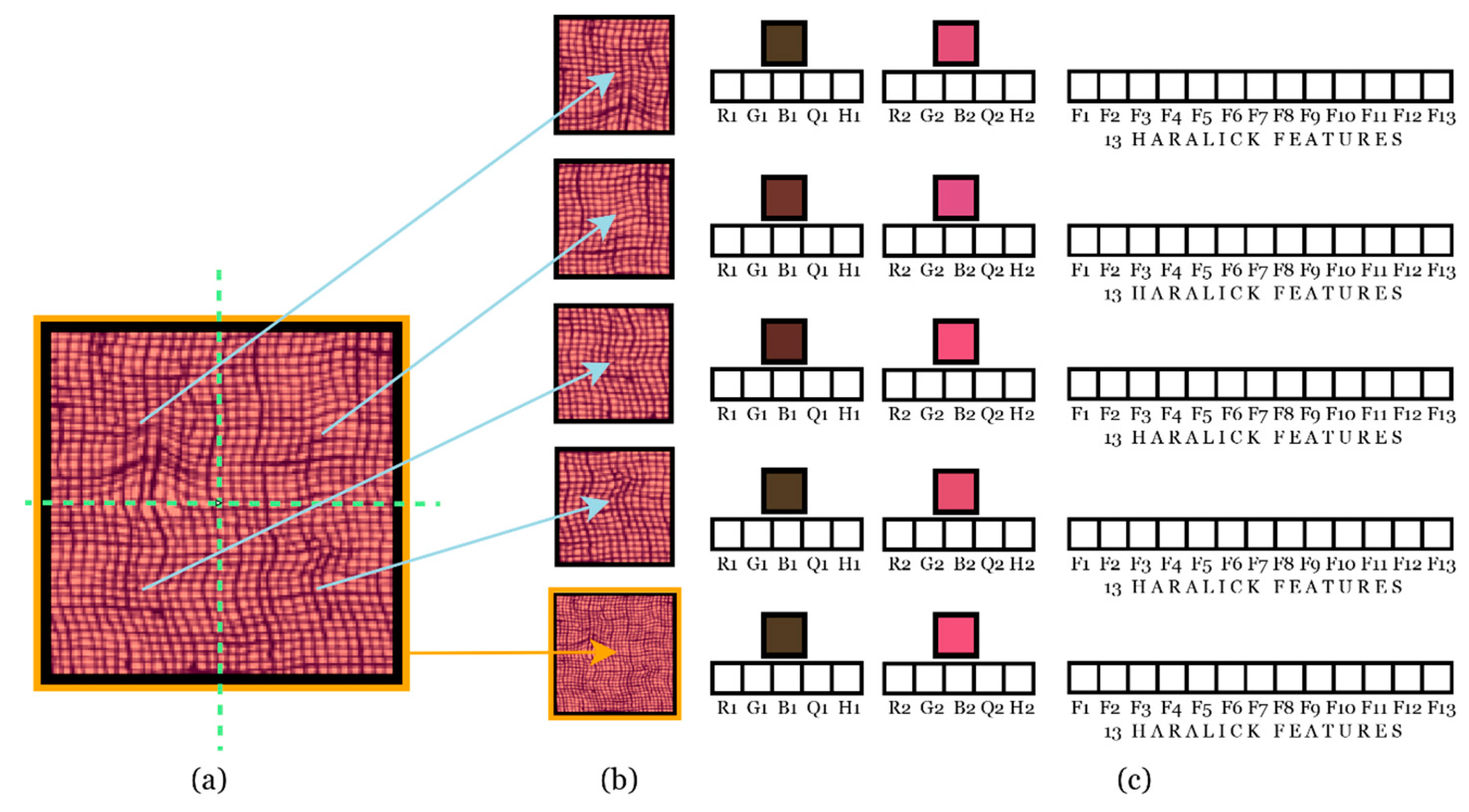
The feature extraction is performed using local and global scales. The feature vector is created by extracting features from each different image partition (local and global). An example is shown in Figure 7. The original image (a) is divided into five partitions, (b) four local and one global (the same original image), as shown in Figure 4. The feature vector is obtained from each partition as shown in (c). Since BQMP is applied once, we obtain different values for two representative colors for each sub-image. As in the example shown in Figure 7c, the first representative color is brown with R1 = 78, G1 = 62, and B1 = 39. The other color is pink with R2 = 215, G2 = 80, B2 = 119. Through binarization, we know that brown represents 41% of the image and pink 59%; therefore, H1 = 0.41 and H2 = 0.59.
To achieve the binarization, the three-dimensional RGB information was transformed in a four-dimensional quaternion. Those quaternions were used to obtain the moments of order 1, 2, and 3, and the moments were used to obtain the equations of momentum conservation, to obtain the representative colors (R1,G1,B1 and R2,G2,B2) and the representative histograms (H1 and H2), as Reference [6] described. The moments were computed using quaternion multiplication that is a four-dimensional operation. For example, in the case of two quaternions a = a 1 + a 2 i + a 3 j + a 4 k and b = b 1 + b 2 i + b 3 j + b 4 k , the product will be equal to a b = ( a 1 b 1 a 2 b 2 a 3 b 3 a 4 b 4 ) + ( a 1 b 2 + a 2 b 1 + a 3 b 4 a 4 b 3 ) i +   ( a 1 b 3 a 2 b 4 + a 3 b 1 + a 4 b 2 ) j + ( a 1 b 4 + a 2 b 3 a 3 b 2 + a 4 b 1 ) k . Therefore, even if a 1 and b 1 are equal to zero, the real part of the multiplication will not necessarily be zero. In the case of the example, this extra information is Q1 = −0.61 in the first color and Q2 = 0.43 in the second color.
Then, we extracted the 13 Haralick features (explained in Section 2.3) in each sub-image and each color channel, obtaining 13 × 5 × 3 = 195 more features to concatenate into the final vector.
In the texture of Figure 7, we performed only one BQMP iteration in an image from Brodatz database, obtaining only two color representatives. In general, the BQMP method generates 2n representatives from each image, when n iterations are used. In Figure 5 and Figure 6, an example for a simple color pattern shows the representatives for two iterations, n = 2. In our preliminary experiments, the results did not improve significantly for n ≥ 3, and computational time increased significantly. The feature extraction was performed in local and global scales, so that the representative colors would capture the diversity of the whole image in a local and global manner.
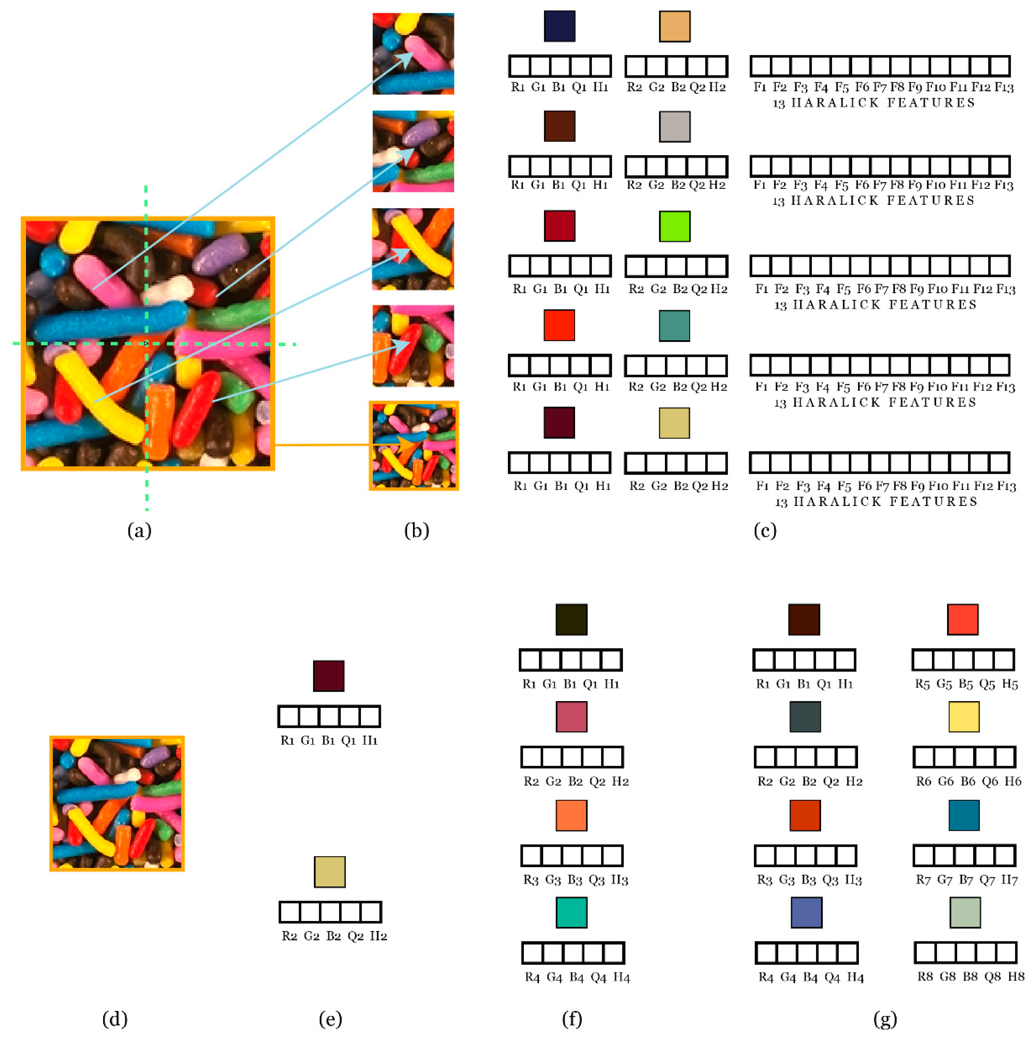
In the case of more complex textures, it is possible to use more iterations of the BQMP method obtaining more representative colors, histograms, and quaternions. Figure 8 shows the feature extraction from one sample image from the Vistex database (Food0007) using one, two, or three iterations of the method.
As in the example shown in Figure 8c, the first representative color is dark blue with R1 = 30, G1 = 32, and B1 = 69. The other color is cream with R2 = 217, G2 = 172, and B2 = 106. Through binarization, we know that dark blue represents 74% of the image and cream 26%; therefore, H1 = 0.74 and H2 = 0.26. Q1 and Q2 are 1.49 and −2.43, respectively. The Haralick features computed from Equations (1)–(13) for the first sub-image are the following: F1 = 1.09 × 10⁻⁴, F2 = 2.66 × 10³, F3 = 9.90 × 10⁸, F4 = 4.75 × 10³, F5 = 2.60 × 10⁻², F6 = 1.24 × 10², F7 = 1.65 × 10⁴, F8 = 5.28, F9 = 9.32, F10 = 2.43 × 10⁻⁵, F11= 4.63, F12 = −6.37 × 10⁻², and F13 = 6.78 × 10⁻¹.

2.5. SVM Classifier and Post-Processing

After features were extracted from each image, an SVM classifier was used to determine each texture class. The SVM became very popular within the machine learning community due to its great classification potential [41,42]. The SVM maps input vectors in a non-linear transformation to a high-dimensional space where a linear decision hyperplane is constructed for class separation. A Gaussian SVM kernel was used, and a coarse exhaustive search over the remaining SVM parameters was performed to find the optimal configuration on the training set.
A grid search with cross-validation was used to find the best parameters for the multiclass SVM cascade. We used half of the training set to determine the SVM parameters, and the other half in validation. For testing, we used a different set as explained in Section 3.1. In the case of bagging, we took repeated samples from the original training set for balancing the class distributions to generate new balanced datasets. Two parameters were tuned: the number of decision trees voting in the ensemble, and the complexity parameter related to the size of the decision tree. The method was trained for texture classification using the training sets as they are specified for each database.
In order to have a fair comparison between our obtained classification rates and those previously published, we employed the same partitions used for training and testing as in Diaz-Pernas et al., 2011 [1], Khan et al., 2015 [7], Arvis et al., 2004 [9], Mäenpää et al., 2004 [27], Qazi et al., 2011 [28], Losson et al., 2013 [4], and Couto et al., 2017 [50]. The training and test sets came from separate sub-images, and the methods never used the same sub-image for both training and testing.
In general, combining multiple classification models increases predictive performance [51]. In the post-processing stage, a bagging predictive model composed of a weighted combination of weak classifiers was performed with the results of the SVM model [52]. Bagging is a technique which uses bootstrap sampling to reduce the variance and improve the accuracy of a predictor [51]. It may be used in classification and regression. We created a bagging ensemble for classification using deep trees as weak learners. The bagging predictor was trained with new images taken from the training set of each database. This result was assigned as the final classification for each image.
We compared our results with those published previously on the same databases.

2.6. Databases

It is important to validate the method on standard colored texture databases with previously published results [53]. Therefore, we chose four colored texture databases that were used recently for this purpose: the Colored Brodatz Texture (CBT) [20], Vistex [4], Outex [47], and KTH-TIPS2b [48] databases.
The Brodatz Colored Texture (CBT) database has 111 images of 640 × 640 pixels. Each image in the database has a different texture. The Vistex Database was developed at Massachusetts Institute of Technology (MIT). It has 54 images of 512 × 512 pixels. Each image in the database has a natural color texture. The Outex Database was developed at the University of Oulu, Finland. We used 68 color texture images of 746 × 538, to obtain 1360 images of 128 × 128 with 68 different textures. Each image in the database has a natural color texture. Finally, the KTH-TIPS2b database contains images of 200 × 200 pixels. It has four samples of 108 images of 11 materials at different scales. Each image in the database has a natural color texture.

3. Results

3.1. Experiments

In order to have a fair comparison between our obtained classification rates and those previously published, we used the same databases and partitions used for training and testing as in Diaz-Pernas et al., 2011 [1], Khan et al., 2015 [7], Arvis et al., 2004 [9], Mäenpää et al., 2004 [27], Qazi et al., 2011 [28], Losson et al., 2013 [4], and Couto et al., 2017 [50]. The training and test sets came from separate sub-images, and the methods never used the same sub-image for both training and testing.

3.1.1. Brodatz Database

The methodology, as in Reference [1], used four different sets of images from the same database: the first one consisted of 10 images, the second of 30 images, the third of 40 images, and the fourth of all 111 images. The classification results in previously published articles reached 91.03% in Reference [1], 89.71% in Reference [43], and 88.15% in Reference [44] for the fourth set of the Brodatz database. We used the same partition used for training and testing as in Diaz-Pernas et al., 2011 [1]. The Brodatz image database consists of 111 images of size 640 × 640 pixels. Partitioning each image into nine non overlapping sub-images of 213 × 213 pixels, we obtained 999 sub-images from 111 texture classes. Diaz-Pernas et al., 2011 [1], using the (2 × 2) center sub-image as training and the other to test, reached the best classification results (see Figure 2).
In training, each training sub-image with a size of 213 × 213 pixels was subdivided into a number n of images. Features were extracted from each subdivided image. The parameter n changed from 2 to 7 in the first three experiments, and from 2 to 9 in the last one. Once the feature vector was computed, each vector was assigned to a texture class using an SVM as a classifier.

3.1.2. Vistex Database

The methodology used 54 images that were subdivided into 864 sub-images; 432 were used in training and the other 432 as testing images, as in Arvis et al., 2004 [9], Mäenpää et al., 2004 [27], Qazi et al., 2011 [28], Losson et al., 2013 [4], and Couto et al., 2017 [50]. Previously published results reached 98.61% and 99.07% [4] on the same database using color filter array (CFA) chromatic co-occurrence matrices (CCM). We chose the same 54 texture images to be able to compare our results with those previously published.

3.1.3. Outex Database

The methodology used 68 images that were subdivided into 1360 sub-images; 680 were used in training and the other 680 as testing images, as in Arvis et al., 2004 [9]. The same partition was performed by Mäenpää et al., 2004 [27], Qazi et al., 2011 [28], Losson et al., 2013 [4], and Couto et al., 2017 [50]. Previously published results reached 94.85% and 94.41% [4] on the same database using CFA chromatic co-occurrence matrices. We chose the same 68 texture images and partition to be able to compare our results with those previously published.

3.1.4. KTH-TIPS2b Database

The KTH-Tips2b database consists of four sets of 1,188 images. Each set has 11 different classes. The methodology used four sets of 108 images, each one with 11 images, making a total of 1188 images. We followed the same protocol described in Reference [7], where the average classification performance was reported over four test runs. In each run, all images from one sample were used for training, while all the images from the remaining three samples were used for testing as in Khan et al., 2015 [7]. Previously published results reached 70.6% [7] and 91.3% [8] on the same database using Divisive Information Theoretic Clustering (DITC) and three-dimensional adaptive sum and difference (3D-ASDH) methods, respectively.

3.2. Results

3.2.1. Brodatz Database

Table 1 shows the classification results for the Brodatz database. In this experiment, we used the features extracted in the first set (10 images), varying the size of the images in training r × n2. The last column shows the results of using the post-processing stage applied on the column with the best performance. The best result for the first experiment on the Brodatz database using 10 images was 100%. In this case, 27 (3 × 32) images with size 71 × 71 (213/3) pixels were used for training. It can also be observed that the use of the post-processing step improved the results up to 100% in all cases. These results were higher than 98.23%, the best result previously published for this experiment on the Brodatz database [1]. Also, Table 1 shows the classification results for the second, third, and fourth experiments on the Brodatz database with 30, 40, and 111 images, respectively. The best result reached using 30 images was 99.84%. In this case, 64 (4 × 42) random images with size 53 × 53 (213/4) pixels were used for training. It can also be observed that the use of the post-processing step improved the results up to 100% in all cases. These results are higher than the best result, 97.54%, previously published for this experiment on the Brodatz database [1].
The best result reached using 40 images was 99.71%. In this case, 100 (4 × 52) random images of size 42 × 42 (213/5) pixels were used for training. It can also be observed that the use of the post-processing step improved the results up to 100% in all cases. These results are higher than 95.5%, the best previously published result for this experiment on the Brodatz database [1]. The best result reached using all the 111 images was 97.63%. In this case, 196 (4 × 72) random images of size 30 × 30 (213/7) pixels were used for training. It can also be observed that the use of the post-processing step improved the results up to 99.88%. These results are higher than the bests result of 98.25% and 99.5% previously published for this experiment on the Brodatz database [30,50].
The size of the smaller images reached an optimum for n = 7 with an image size of 30 × 30. We performed an exhaustive search varying from n = 2 to n = 9, reaching an optimum at n = 7. An explanation is that n = 7 is optimal for the complete method using texture and color features. Table 2 compares the results previously published in the literature and our results on the Brodatz database for the four experiments which included 10, 30, 40, and 111 images, respectively.
It can be seen in Table 2 that our method, with post-processing, reached the highest results. The most significant improvement was reached on the complete Brodatz database that includes 111 images.

3.2.2. Vistex Database

Table 3 shows the classification results of our method applied to the Vistex database (54 images). Each image in the training set was partitioned randomly, and the number of windows per side was varied from two to four in each image chosen for training, with the number of random images from 4 × n2 to 10 × n2. The first column shows the best results reached by our method, and the second column shows the results after the post-processing stage. Table 4 compares the results published previously in the literature and our results for the Vistex database with 54 images. It can be observed in Table 4 that our post-processed method reached the highest results with 100%.

3.3.3. Outex Database

Table 5 shows the classification results of our method applied to the Outex database (68 images). Each image in the training set was partitioned randomly, varying the number of windows per side from two to four in each training image, and the number of random images from 5 × n2 to 18 × n2. The first column shows the best results reached by our method, and the second column shows the results after the post-processing stage. The best results are highlighted by bold text.
Table 6 compares the results published previously in the literature and our results for the Outex database with 68 images. It can be observed in Table 6 that our post-processed method reached the highest results with 98.97%.

3.3.4. KTH-TIPS2b Database

Table 7 shows the classification results of our method applied to the KTH-TIPS2b database (1188 × 4 images). In each test, all the images from one sample were used for training, while the images from the remaining three samples were used as a test set. The first column shows the best results reached by our method, and the second column shows the results after the post-processing stage.
Table 8 compares the results published previously in the literature and our results for the KTH-TIPS2b database with 1188 × 4 images. It can be observed in Table 8 that our post-processing method reached the highest results with 95.75%.

3.3.5. Color or Texture vs. Color and Texture

Table 9 compares the results of color features, texture features, and of the combination of both, for texture classification measured on the Brodatz, Vistex, Outex, and KTH-TIPS2b databases. It can be observed that both types of features, color and texture, contribute to the overall results, with maximum performance when both types of features are combined. Comparing these results to those previously published on the same databases, it can be observed that, although the method reached 100% on the Vistex database in Reference [28], the results yielded on Outex were only 94.5%.

3.3.6. Computation Time

Table 10 displays the computational time required for feature extraction (FE), classification time with the SVM, and post-processing (PP) time performed on the Vistex database. All implementations were carried out using Python 3 on an Intel (R) Core (TM) i7-7700HM 3.6 GHz, with 64 GB of random-access memory (RAM).

4. Discussion

The idea of combining color and texture was proposed previously, but the proposed feature extraction process allows the method to preserve the information available in the original image, yielding significantly better results than those previously published. A possible drawback of previous texture classification methods is that important information is lost from the original image with the feature extraction method, hampering its ability to improve texture classification results. The feature extraction process that includes global and local features is something new from the point of view of combining color with texture. Sub-dividing the training partition of the database into sub-images, and trying to obtain all the information present in the image using various image sizes or a different number of images is something that was not reported in previous publications.
Color and texture features are extracted in order to classify complex colored textures. However, the feature extraction process loses part of the information present in the image because the two-dimensional (2D) information is transformed into a reduced space. By using global and local features extracted from many different partitions of the image, the information needed for colored texture classification is preserved better. Sub-dividing the training data into sub-images (local–global) and trying to obtain all the information present using different image sizes is a new approach.
Although the BQMP method was proposed several years ago [6], it was used in color data compression, color edge detection, and multiclass clustering of color data. The reduction of an image into representative colors and a histogram that indicates which part of the image is represented by these colors achieves excellent results. In addition, local and global features are extracted from each image. The results of our method were compared with those of several other feature extraction implementations on the Brodatz database with those published in References [1,27,28,31,43,44,50], on the Vistex database with those published in References [4,9,13,23,27,28,30,38,45,46,50], on the Outex database with those published in References [4,8,9,11,27,28,30,38,45,46,50], and on the KTH-TIPS2b with those published in References [7,8,31,34,35] (please see Table 2, Table 4, Table 6 and Table 8). The proposed method generated better results than those that were published previously.
The databases Brodatz, Vistex, Outex, and KTH2b-Tips are available for comparing the results of different texture classification methods. Tests should be performed under the same conditions. We compared our results with those of References [1,7] under the same conditions using the same training/test distribution, and an SVM as a classifier. We also compared our results with those of Reference [4] in which they used a nearest-neighbor classifier (KNN) and, therefore, we tested our method with KNN instead of SVM. The results with KNN are shown in Table 2, Table 4, Table 6 and Table 8, corroborating that SVM achieves better results. The proposed method achieved better results than those previously published.

5. Conclusions

In this paper, we presented a new method for classifying complex patterns of colored textures. Our proposed method includes four main steps. Firstly, the image is divided into local and global images. This image sub-division allows feature extraction in different spatial scales, as well as adding spatial information to the extracted features. Therefore, we capture global and local features from the texture. Secondly, texture and color features are extracted from each divided image using the BQMP and Haralick algorithms. Thirdly, a support vector machine is used to classify each image with the extracted features as inputs. Fourthly, a post-processing stage using bagging is employed.
The method was tested on four databases, the Brodatz, VisTex, Outex, and KTH-TIPS2B databases, yielding correct classification rates of 97.63%, 97.13%, 90.78%, and 92.90% respectively. The post-processing stage improved the results to 99.88%, 100%, 98.97%, and 95.75%, respectively, for the same databases. We compared our results on the same databases to the best previously published results finding significant improvements of 8.85%, 0.93% (to 100%), 4.12%, and 4.45%.
The partition of the image into local and global images provides information about features at different scales and spatial locations within each image, which is useful in color/texture classification. The above, combined with the use of a post-processing stage using a bagging predictive model, allows achieving such results.

Author Contributions

Conceptualization, C.F.N. and C.A.P.; methodology, C.F.N. and C.A.P.; software, C.F.N.; validation, C.F.N. and C.A.P.; formal analysis, C.F.N. and C.A.P.; investigation, C.F.N. and C.A.P.; resources, C.A.P.; data curation, C.F.N.; Writing—Original Draft preparation, C.F.N. and C.A.P.; Writing—Review and Editing, C.F.N. and C.A.P.; visualization, C.F.N.; supervision, C.A.P.; project administration, C.A.P.; funding acquisition, C.A.P.

Funding

This research was funded by FONDECYT, grant number 1191610 from CONICYT, the Department of Electrical Engineering, and the Advanced Mining Technology Center, Universidad de Chile.

Conflicts of Interest

The authors declare no conflict of interest.

References

  1. Díaz-Pernas, F.J.; Antón-Rodríguez, M.; Perozo-Rondón, F.J.; González-Ortega, D. A multi-scale supervised orientational invariant neural architecture for natural texture classification. Neurocomputing 2011, 74, 3729–3740. [Google Scholar] [CrossRef]
  2. Drimbarean, A.; Whelan, P.F. Experiments in colour texture analysis. Pattern Recognit. Lett. 2001, 22, 1161–1167. [Google Scholar] [CrossRef] [Green Version]
  3. Haralick, R.M.; Shanmugam, K.S.; Dinstein, I. Textural Features for Image Classification. IEEE Trans. Syst. Man Cybern. 1973, 3, 610–621. [Google Scholar] [CrossRef]
  4. Losson, O.; Porebski, A.; Vandenbroucke, N.; Macaire, L. Color texture analysis using CFA chromatic co-occurrence matrices. Comput. Vis. Image Underst. 2013, 117, 747–763. [Google Scholar] [CrossRef]
  5. Ojala, T.; Pietikainen, M.; Harwood, D. Performance evaluation of texture measures with classification based on Kullback discrimination of distributions. In Proceedings of the 12th International Conference on Pattern Recognition, Jerusalem, Israe, 9–13 October 1994; Volume 1, pp. 582–585. [Google Scholar]
  6. Pei, S.C.; Cheng, C.M. Color image processing by using binary quaternion-moment-preserving thresholding technique. IEEE Trans. Image Process. 1999, 8, 614–628. [Google Scholar]
  7. Khan, F.S.; Anwer, R.M.; van de Weijer, J.; Felsberg, M.; Laaksonen, J. Compact color-texture description for texture classification. Pattern Recognit. Lett. 2015, 51, 16–22. [Google Scholar] [CrossRef]
  8. Sandid, F.; Douik, A. Robust color texture descriptor for material recognition. Pattern Recognit. Lett. 2016, 80, 15–23. [Google Scholar] [CrossRef]
  9. Arvis, V.; Debain, C.; Berducat, M.; Benassi, A. Generalization of the cooccurrence matrix for colour images: Application to colour texture classification. Image Anal. Stereol. 2011, 23, 63–72. [Google Scholar] [CrossRef]
  10. Bianconi, F.; González, E.; Fernández, A.; Saetta, S.A. Automatic classification of granite tiles through colour and texture features. Expert Syst. Appl. 2012, 39, 11212–11218. [Google Scholar] [CrossRef]
  11. Bianconi, F.; Harvey, R.W.; Southam, P.; Fernández, A. Theoretical and experimental comparison of different approaches for color texture classification. J. Electron. Imaging 2011, 20, 043006. [Google Scholar] [CrossRef]
  12. Cament, L.A.; Galdames, F.J.; Bowyer, K.W.; Perez, C.A. Face recognition under pose variation with local Gabor features enhanced by Active Shape and Statistical Models. Pattern Recognit. 2015, 48, 3371–3384. [Google Scholar] [CrossRef]
  13. Hiremath, P.S.; Shivashankar, S.; Pujari, J. Wavelet based features for color texture classification with application to cbir. Int. J. Comput. Sci. Netw. Secur. 2006; 6, pp. 124–133. [Google Scholar]
  14. Perez, C.A.; Aravena, C.M.; Vallejos, J.I.; Estevez, P.A.; Held, C.M. Face and iris localization using templates designed by particle swarm optimization. Pattern Recognit. Lett. 2010, 31, 857–868. [Google Scholar] [CrossRef]
  15. Perez, C.A.; Cament, L.A.; Castillo, L.E. Methodological improvement on local Gabor face recognition based on feature selection and enhanced Borda count. Pattern Recognit. 2011, 44, 951–963. [Google Scholar] [CrossRef]
  16. Perez, C.A.; Saravia, J.A.; Navarro, C.F.; Schulz, D.A.; Aravena, C.M.; Galdames, F.J. Rock lithological classification using multi-scale Gabor features from sub-images, and voting with rock contour information. Int. J. Miner. Process. 2015, 144, 56–64. [Google Scholar] [CrossRef]
  17. Perez, C.A.; Estévez, P.A.; Vera, P.A.; Castillo, L.E.; Aravena, C.M.; Schulz, D.A.; Medina, L.E. Ore grade estimation by feature selection and voting using boundary detection in digital image analysis. Int. J. Miner. Process. 2011, 101, 28–36. [Google Scholar] [CrossRef]
  18. Nan, B.; Mu, Z.; Chen, L.; Cheng, J. A Local Texture-Based Superpixel Feature Coding for Saliency Detection Combined with Global Saliency. Appl. Sci. 2015, 5, 1528–1546. [Google Scholar] [CrossRef]
  19. Zeng, D.; Zhu, M.; Zhou, T.; Xu, F.; Yang, H. Robust Background Subtraction via the Local Similarity Statistical Descriptor. Appl. Sci. 2017, 7, 989. [Google Scholar] [CrossRef]
  20. Abdelmounaime, S.; Dong-Chen, H. New Brodatz-Based Image Databases for Grayscale Color and Multiband Texture Analysis. Isrn Mach. Vis. 2013, 2013, 1–14. [Google Scholar] [CrossRef]
  21. Ilea, D.E.; Whelan, P.F. Image segmentation based on the integration of colour–texture descriptors—A review. Pattern Recognit. 2011, 44, 2479–2501. [Google Scholar] [CrossRef]
  22. Wang, Y.; Yang, J.; Peng, N. Unsupervised color–texture segmentation based on soft criterion with adaptive mean-shift clustering. Pattern Recognit. Lett. 2006, 27, 386–392. [Google Scholar] [CrossRef]
  23. Barros Neiva, M.; Vacavant, A.; Bruno, O.M. Improving texture extraction and classification using smoothed morphological operators. Digit. Signal Process. 2018, 83, 24–34. [Google Scholar] [CrossRef]
  24. Andrearczyk, V.; Whelan, P.F. Using filter banks in convolutional neural networks for texture classification. Pattern Recognit. Lett. 2016, 84, 63–69. [Google Scholar] [CrossRef]
  25. Zhu, Q.; Zhong, Y.; Liu, Y.; Zhang, L.; Li, D. A Deep-Local-Global Feature Fusion Framework for High Spatial Resolution Imagery Scene Classification. Remote Sens. 2018, 10, 568. [Google Scholar] [Green Version]
  26. Basu, S.; Mukhopadhyay, S.; Karki, M.; DiBiano, R.; Ganguly, S.; Nemani, R.; Gayaka, S. Deep neural networks for texture classification—A theoretical analysis. Neural Netw. 2018, 97, 173–182. [Google Scholar] [CrossRef]
  27. Mäenpää, T.; Pietikäinen, M. Classification with color and texture: Jointly or separately? Pattern Recognit. 2004, 37, 1629–1640. [Google Scholar] [CrossRef]
  28. Qazi, I.-U.-H.; Alata, O.; Burie, J.-C.; Moussa, A.; Fernandez-Maloigne, C. Choice of a pertinent color space for color texture characterization using parametric spectral analysis. Pattern Recognit. 2011, 44, 16–31. [Google Scholar] [CrossRef]
  29. Shi, L.; Funt, B. Quaternion color texture segmentation. Comput. Vis. Image Underst. 2007, 107, 88–96. [Google Scholar] [CrossRef]
  30. Cernadas, E.; Fernández-Delgado, M.; González-Rufino, E.; Carrión, P. Influence of normalization and color space to color texture classification. Pattern Recognit. 2017, 61, 120–138. [Google Scholar] [CrossRef]
  31. Kim, N.C.; So, H.J. Directional statistical Gabor features for texture classification. Pattern Recognit. Lett. 2018, 112, 18–26. [Google Scholar] [CrossRef]
  32. Wang, M.; Gao, L.; Huang, X.; Jiang, Y.; Gao, X. A Texture Classification Approach Based on the Integrated Optimization for Parameters and Features of Gabor Filter via Hybrid Ant Lion Optimizer. Appl. Sci. 2019, 9, 2173. [Google Scholar] [CrossRef]
  33. Backes, A.R.; de Mesquita Sá Junior, J.J. LBP maps for improving fractal based texture classification. Neurocomputing 2017, 266, 1–7. [Google Scholar] [CrossRef]
  34. El merabet, Y.; Ruichek, Y. Local Concave-and-Convex Micro-Structure Patterns for texture classification. Pattern Recognit. 2018, 76, 303–322. [Google Scholar] [CrossRef]
  35. El merabet, Y.; Ruichek, Y.; El idrissi, A. Attractive-and-repulsive center-symmetric local binary patterns for texture classification. Eng. Appl. Artif. Intell. 2019, 78, 158–172. [Google Scholar] [CrossRef]
  36. Hiremath, P.S.; Bhusnurmath, R.A. Multiresolution LDBP descriptors for texture classification using anisotropic diffusion with an application to wood texture analysis. Pattern Recognit. Lett. 2017, 89, 8–17. [Google Scholar] [CrossRef]
  37. Jeena Jacob, I.; Srinivasagan, K.G.; Jayapriya, K. Local Oppugnant Color Texture Pattern for image retrieval system. Pattern Recognit. Lett. 2014, 42, 72–78. [Google Scholar] [CrossRef]
  38. Kalakech, M.; Porebski, A.; Vandenbroucke, N.; Hamad, D. Unsupervised Local Binary Pattern Histogram Selection Scores for Color Texture Classification. J. Imaging 2018, 4, 112. [Google Scholar] [CrossRef]
  39. Shivashankar, S.; Kudari, M.; Hiremath, P.S. Galois Field-based Approach for Rotation and Scale Invariant Texture Classification. Int. J. Image Graph. Signal Process. (Ijigsp) 2018, 10, 56–64. [Google Scholar] [Green Version]
  40. Cortes, C.; Vapnik, V. Support-Vector Networks. Mach. Learn. 1995, 20, 273–297. [Google Scholar] [CrossRef]
  41. Meyer, D.; Leisch, F.; Hornik, K. The support vector machine under test. Neurocomputing 2003, 55, 169–186. [Google Scholar] [CrossRef]
  42. Shang, C.; Barnes, D. Support vector machine-based classification of rock texture images aided by efficient feature selection. In Proceedings of the 2012 International Joint Conference on Neural Networks (IJCNN), Brisbane, QLD, Australia, 10–15 June 2012; pp. 1–8. [Google Scholar]
  43. Lazebnik, S.; Schmid, C.; Ponce, J. A sparse texture representation using local affine regions. IEEE Trans. Pattern Anal. Mach. Intell. 2005, 27, 1265–1278. [Google Scholar] [CrossRef] [Green Version]
  44. Mellor, M.; Hong, B.; Brady, M. Locally Rotation, Contrast, and Scale Invariant Descriptors for Texture Analysis. IEEE Trans. Pattern Anal. Mach. Intell. 2008, 30, 52–61. [Google Scholar] [CrossRef]
  45. Hayati, S.; Ahmadzadeh, M.R. WIRIF: Wave interference-based rotation invariant feature for texture description. Signal Process. 2018, 151, 160–171. [Google Scholar] [CrossRef]
  46. Pham, M.-T.; Mercier, G.; Bombrun, L. Color Texture Image Retrieval Based on Local Extrema Features and Riemannian Distance. J. Imaging 2017, 3, 43. [Google Scholar] [CrossRef]
  47. Ojala, T.; Maenpaa, T.; Pietikainen, M.; Viertola, J.; Kyllonen, J.; Huovinen, S. Outex-new framework for empirical evaluation of texture analysis algorithms. In Proceedings of the Object Recognition Supported by User Interaction for Service Robots, Quebec City, QC, Canada, 11–15 August 2002; Volume 1, pp. 701–706. [Google Scholar]
  48. Caputo, B.; Hayman, E.; Mallikarjuna, P. Class-specific material categorisation. In Proceedings of the Tenth IEEE International Conference on Computer Vision (ICCV’05) Volume 1, Beijing, China, 17–21 October 2005; Volume 2, pp. 1597–1604. [Google Scholar]
  49. Kashyap, R.L.; Khotanzad, A. A Model-based Method for Rotation Invariant Texture Classification. IEEE Trans. Pattern Anal. Mach. Intell. 1986, 8, 472–481. [Google Scholar] [CrossRef]
  50. Couto, L.N.; Backes, A.R.; Barcelos, C.A. Texture characterization via deterministic walks’ direction histogram applied to a complex network-based image transformation. Pattern Recognit. Lett. 2017, 97, 77–83. [Google Scholar] [CrossRef]
  51. Breiman, L. Bagging predictors. Mach. Learn. 1996, 24, 123–140. [Google Scholar] [CrossRef] [Green Version]
  52. Zhang, C.; Ma, Y. Ensemble Machine Learning: Methods and Applications; Springer: Cham, Switzerland, 2012; ISBN 1-4419-9325-8. [Google Scholar]
  53. Hossain, S.; Serikawa, S. Texture Databases—A Comprehensive Survey. Pattern Recogn. Lett. 2013, 34, 2007–2022. [Google Scholar] [CrossRef]
Figure 1. Block diagram of the proposed method.
Applsci 09 03130 g001
Figure 2. (a) The Brodatz image (D88) is used to create the training image (b) and test images (c). (d) The Vistex image (Food0007) is used to create the training images (e) and test images (f). (g) The Outex image (Canvas002) is used to create the training images (h) and test images (i).
Applsci 09 03130 g002
Figure 3. (a) A sample image from Vistex (Food0007) and the subdivision process. (b,e) Image is divided into n2 images. (c,f) Image is divided into n2 random blocks. (d,g) Image is divided into r × n2 random blocks. In this example, (bd) n = 2, (eg) n = 3, and r = 2 (d,g).
Applsci 09 03130 g003
Figure 4. Example of (a) the original image. (b) The four local partitions and (c) the global partition. These five images generate two spatial scales: four local (b) and one global, adding spatial information to the extracted features.
Applsci 09 03130 g004
Figure 5. First binary quaternion-moment-preserving (BQMP) iteration example for the case of four different colors. Numbers show the color coded in (q0, q1, q2, q3) and the number of pixels for each color representative (histogram).
Applsci 09 03130 g005
Figure 6. Second BQMP iteration example for the case of four different colors. Numbers show the color coded in (q0, q1, q2, q3) and the number of pixels for each color representative (histogram).
Applsci 09 03130 g006
Figure 7. Feature vector extracted from one image from the Brodatz Database. (a) The original image is divided into five partitions (b): four local partitions and one global (the same image, bottom). (c) The feature vectors obtained from each partition. The color feature vector and texture feature vector are concatenated.
Applsci 09 03130 g007
Figure 8. Feature vector extracted from one image of the Vistex Database (Food0007). (a) The original image is divided into five partitions (b): four local partitions and one global (the same image, bottom). (c) The feature vectors obtained from each partition. The color feature vectors and texture feature vectors are concatenated. (dg) The global sub-image as a real example using one iteration (e), two iterations (f), or three iterations (g) of the BQMP method.
Applsci 09 03130 g008
Table 1. Classification results of the experiments on the Brodatz database for sets of 10, 30, 40, and 111 images. The best results reached with and without post-processing are highlighted by bold text.
r × n2 Random Images 1 in Training with
No Post-ProcessingPost-Processing
S = 10, r = 3 S = 30, r = 4 S = 40, r = 3 S = 111, r = 4 S = 10, r = 3S = 30, r = 4S = 40, r = 4S = 111, r = 4
n = 299.68%97.71%97.03%87.56%100%100%100%97.07%
n = 3100%99.21%99.38%94.81%100%100%100%99.32%
n = 499.92%99.84%99.67%96.24%100%100%100%99.66%
n = 599.8%99.73%99.71%96.71%100%100%100%99.88%
n = 699.83%99.56%99.70%97.30%100%100%100%99.77%
n = 799.51%99.60%99.61%97.63%100%100%100%99.77%
n = 8 90.05% 99.77%
n = 9 80.31% 96.85%
1 n is the number of images per side in the training stage; r is the times we iterated the method in each image.
Table 2. Best results of global–local Haralick– binary quaternion-moment-preserving (BQMP) classification for the Brodatz database for the four sets of 10, 30, 40, and 111 images compared to previously published studies. SVM—support vector machine.
Best Results vs. Number of Images103040111
Lazebnick et al., 2005 [43]---88.15%
Mellor et al., 2008 [44]---89.71%
Diaz-Pernas et al., 2011 [1]98.23%97.54%95.5%91.03%
Couto el al, 2017 [50]---98.25%
Kim et al., 2017 [31]---97.84%
SVM global–local Haralick BQMP method 1 100%99.84%99.71%97.63%
KNN 2 global–local Haralick BQMP method + post-processing 1100%99.94%99.98%94.46%
SVM global–local Haralick BQMP method + post-processing 1100%100%100%99.88%
1 The last three methods are our results; 2 k-nearest neighbors.
Table 3. Classification results of the experiment on the Vistex database for the set of 54 images. The best results reached with and without post-processing are highlighted by bold text.
r × n2 Random Images 1 in Training
Without Post-ProcessingWith Post-Processing
r = 2r = 3r = 4r = 2r = 3r = 4
n = 495.52%94.83%94.13%99.54%100%100%
n = 595.68%95.29%94.64%99.54%100%100%
n = 696.13%95.88%95.22%100%100%100%
n = 796.45%96.26%95.36%100%100%100%
n = 896.72%96.42%96.42%100%100%100%
n = 995.67%97.13%95.88%100%100%100%
n = 1096.96%96.32%95.62%100%100%100%
1 n is the number of images per side in the training stage; r is the times we iterated the method in each image.
Table 4. Best results of global–local Haralick–BQMP classification for the Vistex database with 54 images and best results published previously on the same database.
PaperMethodResult
Arvis et al., 2004 [9]Multispectral97.9%
Mäenpää et al., 2004 [27]Color histogram I1I2I3323100%
Qazi et al., 2011 [28]Improved hue, luminance, and saturation color space (IHLS) B = 16100%
Losson et al., 2013 [4]Color filter array - chromatic co-occurrence matrices 98.61%
Losson et al., 2013 [4]Chromatic co-occurrence matrices99.07%
Couto et al., 2017 [50]Deterministic walks’ direction histogram 99.65%
Cernadas et al., 2017 [30]Parallel vectors99.5%
Neiva et al., 2018 [23]Smoothed morphological operators (SMO)99.54%
Kalakech et al., 2018 [38]Adapted Laplace score94.9%
Global–local Haralick BQMP method 197.13%
KNN global–local Haralick BQMP method + post-processing 197.25%
Global–local Haralick BQMP method + post-processing 1100%
1 The last three methods are our results.
Table 5. Classification results of the experiment on the Outex database for the set of 68 images. The best results reached with and without post-processing are highlighted by bold text.
r × n2 Random Images 1 in Training
Without Post-ProcessingWith Post-Processing
r = 2r = 3r = 4r = 2r = 3r = 4
n = 587.43%86.46%85.40%97.50%97.79%97.79%
n = 688.49%86.72%85.72%97.50%98.08%98.08%
n = 788.84%86.37%86.15%97.94%97.50%98.08%
n = 889.19%87.44%86.27%98.23%97.79%98.38%
n = 989.38%87.73%86.51%98.67%97.79%98.23%
n = 1089.61%87.96%86.62%97.94%98.23%97.94%
n = 1190.12%88.20%86.85%97.94%98.23%97.94%
n = 1290.35%88.37%87.04%98.97%97.94%98.52%
n = 1390.52%88.50%87.22%98.82%98.38%97.05%
n = 1490.58%88.21%87.38%98.67%97.20%97.20%
n = 1590.78%88.06%86.53%98.67%97.79%96.32%
n = 1690.19%86.92%86.24%97.94%96.62%96.03%
n = 1789.98%86.02%85.10%97.50%96.32%95.44%
n = 1890.18%85.54%84.16%97.64%95.59%94.85%
1 n is the number of images per side in the training stage; r is the times we iterate the method in each image.
Table 6. Best results of global–local Haralick–BQMP classification for the Outex database with 68 images. The best previously published results are compared to our results.
PaperMethodResult
Arvis et al., 2004 [9]Multispectral94.9%
Mäenpää et al., 2004 [27]Color histogram HSV16395.4%
Bianconi et al., 2011 [11]Gabor and chromatic features90.0%
Qazi et al., 2011 [28]IHLS color space B = 1694.5%
Losson et al., 2013 [4]Color filter array - chromatic co-occurrence matrices94.41%
Losson et al., 2013 [4]Chromatic co-occurrence matrices94.85%
Sandid et al., 2016 [8]three-dimensional adaptive sum and difference histograms (3D-ASDH)95.8%
Couto el al, 2017 [50]Deterministic walks direction histogram 97.28%
Neiva et al., 2018 [23]Smoothed morphological operators (SMO)86.47%
Cernadas et al., 2017 [30]Parallel vectors90.6%
Global–local Haralick BQMP method 190.78%
KNN global–local Haralick BQMP method + post-processing 196.72%
Global–local Haralick BQMP method + post-processing 198.97%
1; 1 the last three methods are our results.
Table 7. Classification results of the experiment on the KTH-TIPS2b database for the four sets of 1188 images.
n 2 Random Images 1 in Training
Without Post-ProcessingWith Post-Processing
n = 1n = 2n = 1n = 2
S = 198.73%99.16%99.73%99.65%
S = 292.72%91.26%95.79%95.59%
S = 390.74%88.99%94.53%93.71%
S = 489.42%87.88%92.93%92.89%
Mean92.90%91.82%95.75%95.46%
1 n is the number of images per side in the training stage; S is the set used for training, using the other three sets as test.
Table 8. Best results of global–local Haralick–BQMP classification for the KTH-TIPS2b database with 1188 images per set and the best previously published results on the same database.
PaperMethodResult
Khan et al., 2015 [7]Divisive information theoretic clustering (DITC)70.6%
Sandid et al., 2016 [8]3D-ASDH91.3%
El Merabet et al., 2018 [34]Local concave/convex micro-structure pattern84.44%
El Merabet et al., 2019 [35]Attractive-and-Repulsive Center-Symmetric -LBP93.61%
Global–local Haralick BQMP method 192.90%
KNN global–local Haralick BQMP method + post-processing 192.72%
Global–local Haralick BQMP method + post-processing 195.75%
1 The last three methods are in this paper.
Table 9. Best results of global–local Haralick–BQMP classification for the all databases with the contribution of each part of the model (color and spatial structure).
DatabaseGlobal–Local Haralick BQMP Method with All FeaturesGlobal–Local Haralick BQMP Method with Only Color FeaturesGlobal–Local Haralick BQMP Method with Only Texture Features
Brodatz99.88%96.28%87.84%
Outex98.97%91.86%88.57%
Vistex100%95.67%90.84%
KTH-TIPS2b95.75%94.95%92.59%
Table 10. Computational time of the proposed method on feature extraction (FE), SVM classification time, postprocessing (PP) time and total time. Experiments were conducted on the Vistex database (54 images).
VistexFE Time (s)SVM Time (s)PP Time (s)Total Time (s)
Training 57.05 s 305.19 s44.96 s102.86 s
Test55.88 s41.22 s5.76 s407.2 s
Total112.93 s346.41 s50.72 s510.06 s

