Research on the Damage Evolution Process of Steel Wire with Pre-Corroded Defects in Cable-Stayed Bridges

Abstract
:1. Introduction
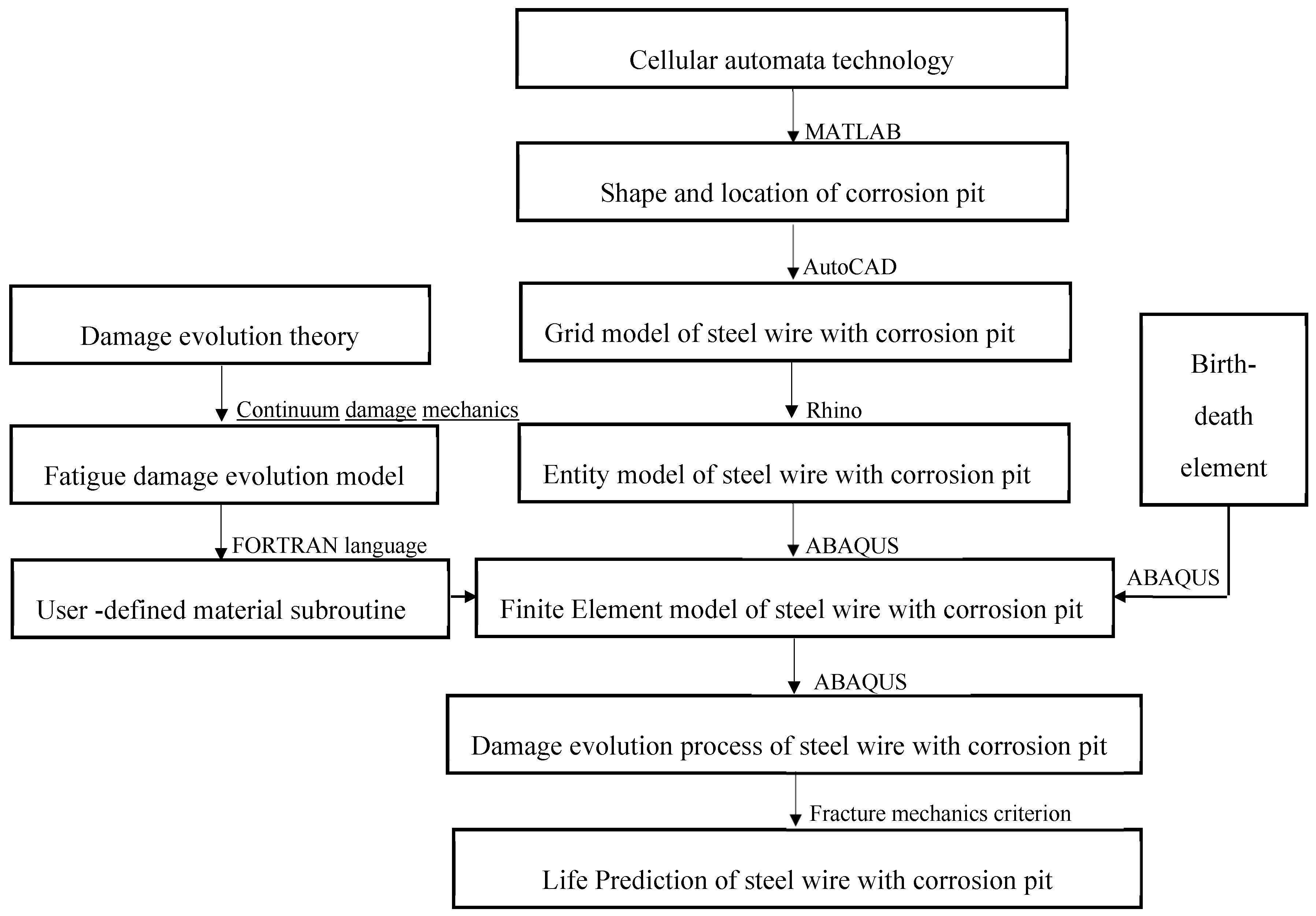
2. Method Proposed
2.1. Fatigue Damage Model of Bridge Wires Based on CDM
2.2. Simulation of the Initial Damage by Using Cellular Automata (CA)
- (1)
- Metal cell (M): the metal cell can be etched away by the corrosive cell, and its position remains unchanged throughout the simulation;
- (2)
- Passive film cell (P): in the CA model, the passive film cell will cover the outermost metal cell initially. The position of the passive film cell is basically fixed, but the initial defect will randomly appear during the simulation, when the passive film cell at the position is converted into a metal cell;
- (3)
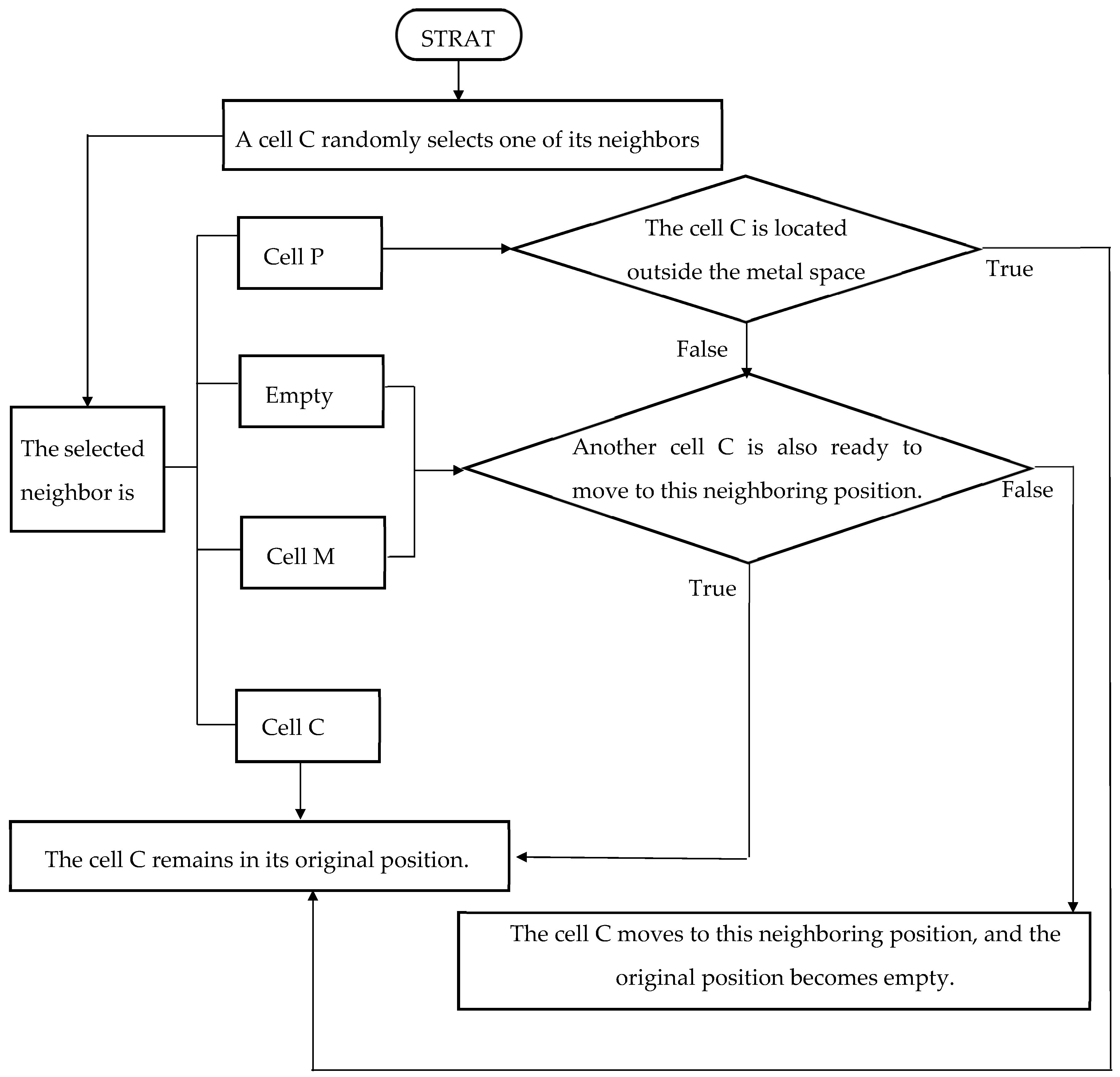
- Corrosive cell (C): The corrosive cell is randomly distributed in solution and the concentration of the corrosive solution is set to 0.1. It can corrode the metal cell and move freely. In the cell space, the corrosive cell can randomly select to move along one direction of coordinate axis in each time step. That is to say, a 6-neighbor type is chosen.
- (1)
- Random diffusion of corrosive media in solution. In the CA model, within a time step, a cell C randomly selects one of its neighbors and is ready to move to the neighboring position. If the selected neighbor position is empty, the cell C jumps to the neighbor cell.
- (2)
- Metal dissolution. It is assumed that Equation (4) does not alter the acidity or alkalinity of the solution in the region. Therefore, in the cellular space, Equation (4) can be expressed as:which indicates that when the metal dissolves, the current position of the cell M is occupied by the cell C of the neighboring position, and then the corresponding neighboring position becomes empty.
- (3)
- Breakage of the passive film on the metal surface. In the CA model, if the selected neighbor is a cell P and the cell C is not located outside the metal space, the cell P will convert to a cell M, i.e.,and then the cell M is corroded by the cell C as the Equation (5); while if the selected neighbor is a cell P but the cell C is located outside the metal space, the cell C remains its original position.
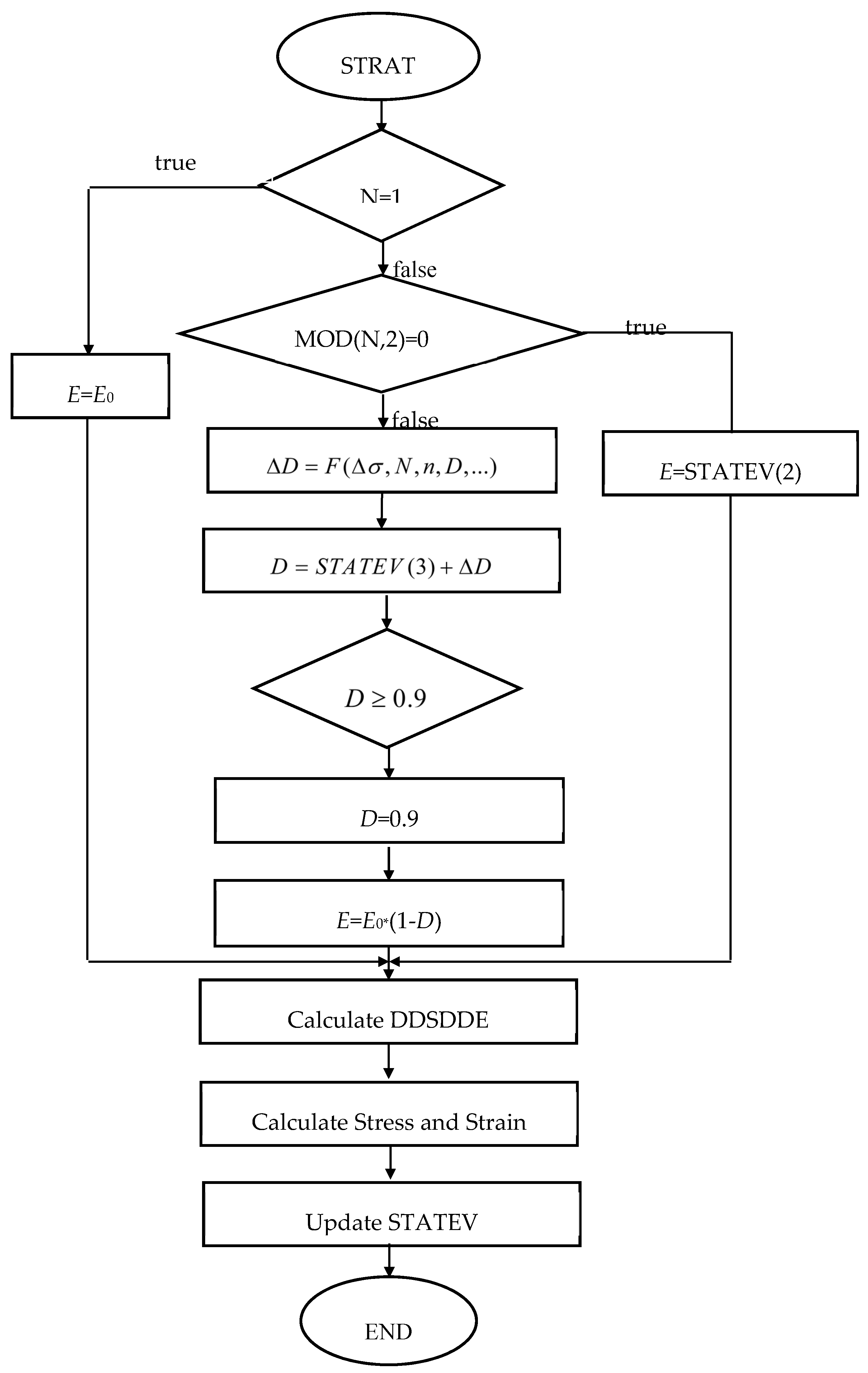
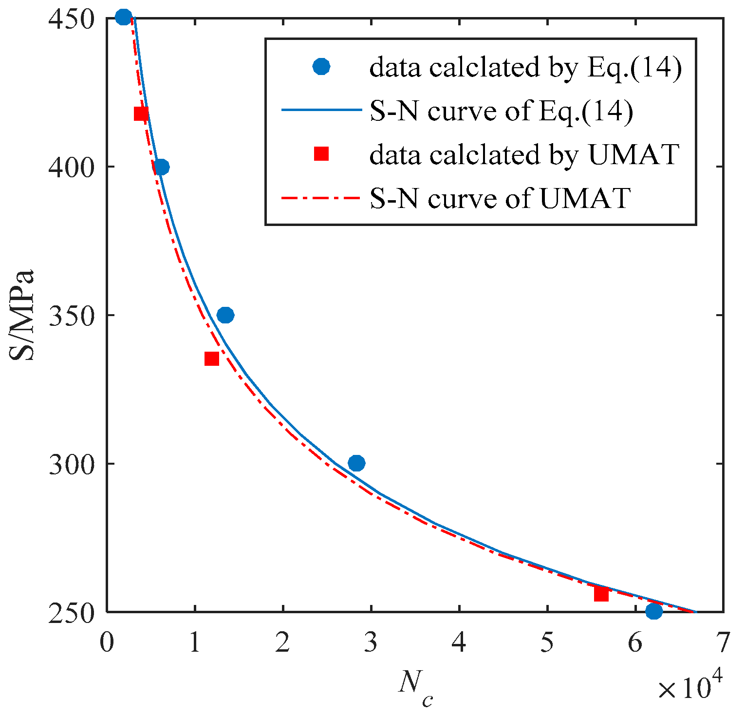
2.3. Fatigue Damage Simulation Algorithm (UMAT)
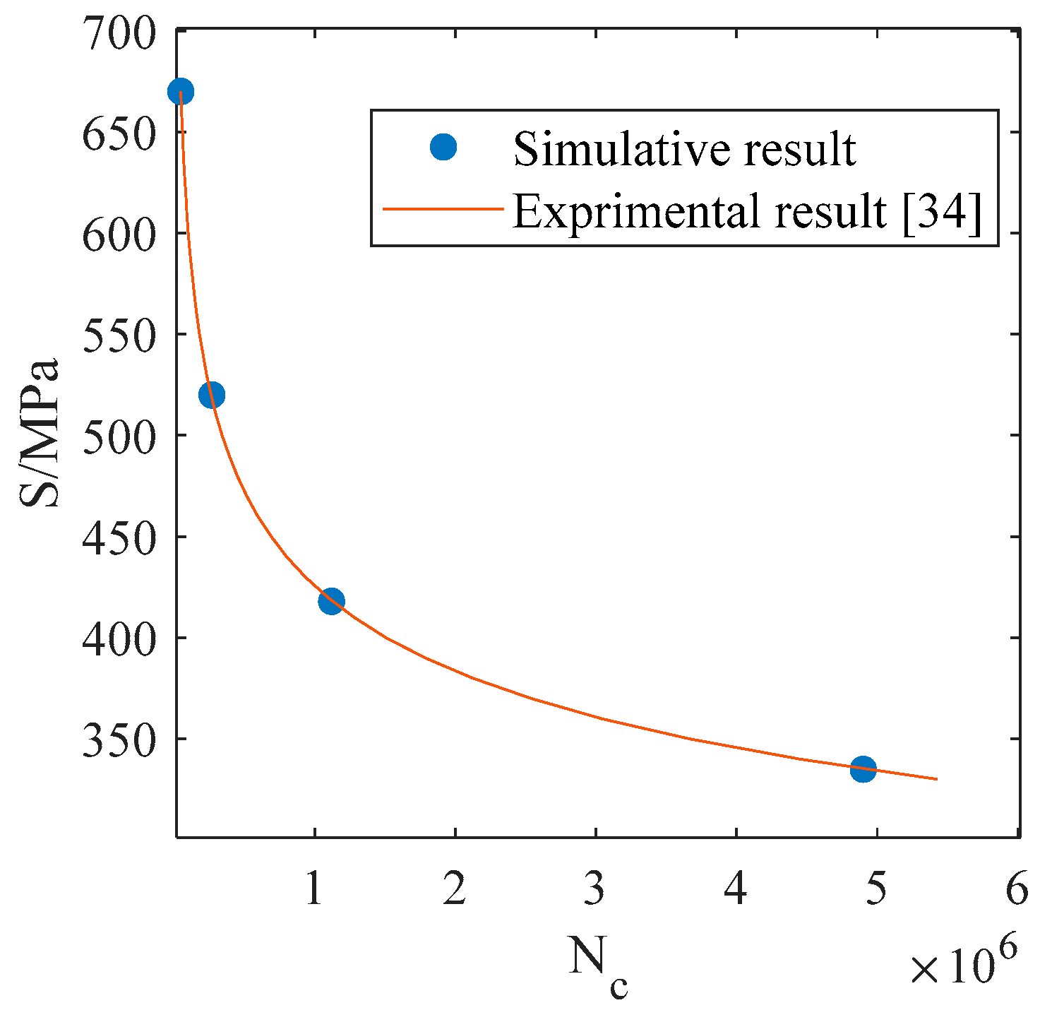
2.4. Verification of the Proposed Method
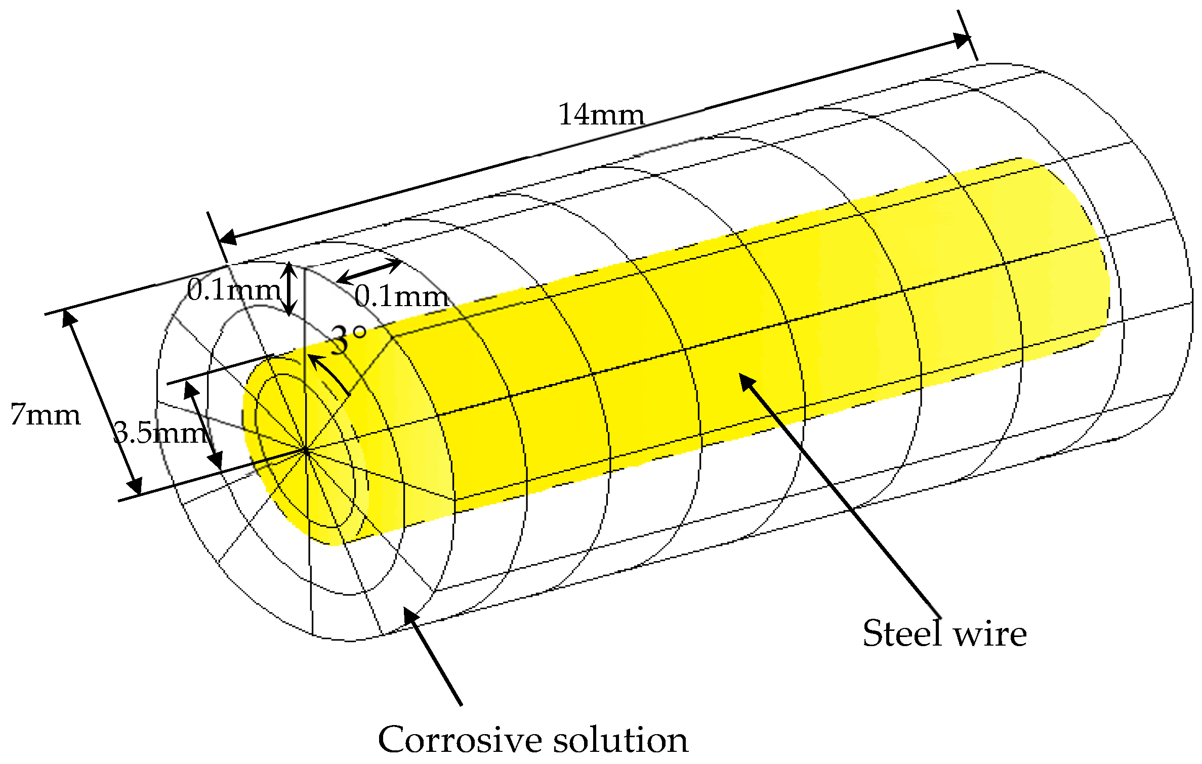
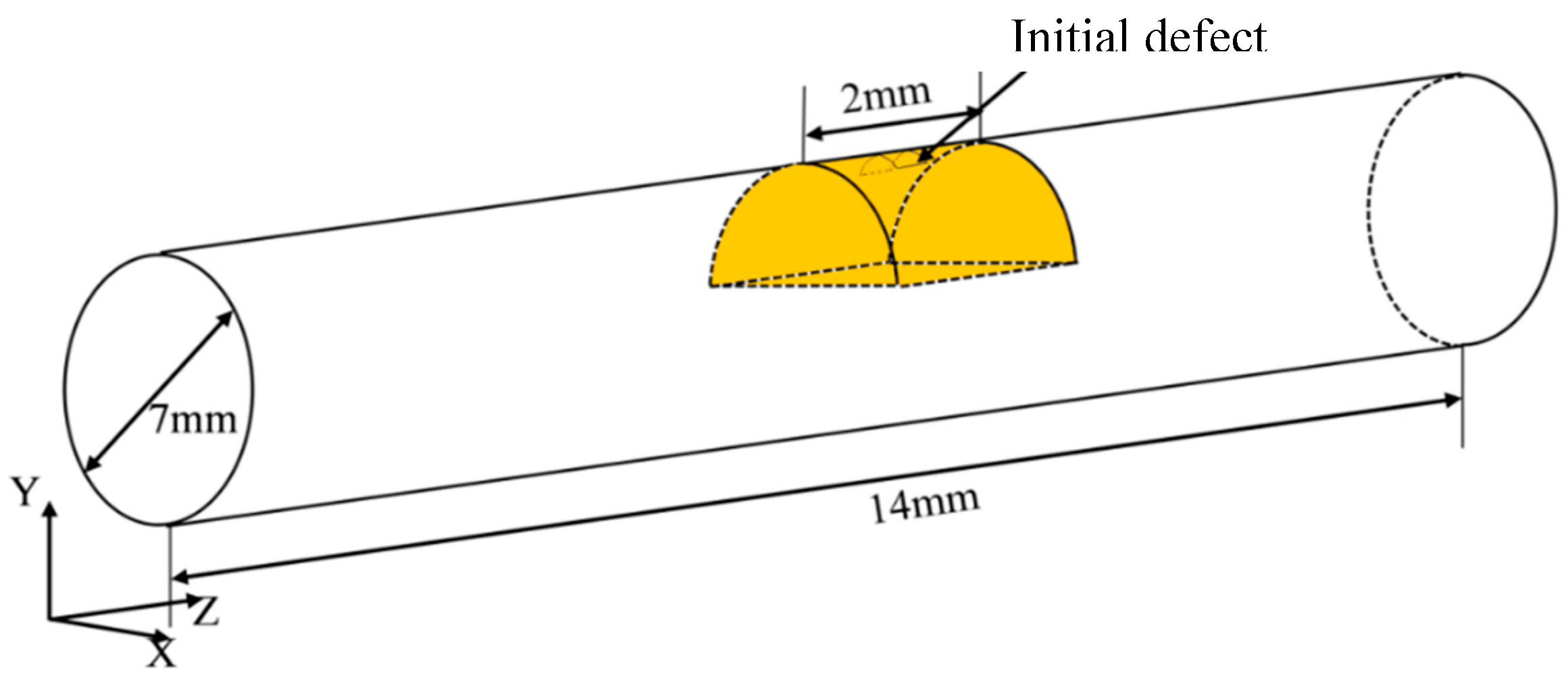
3. Examples
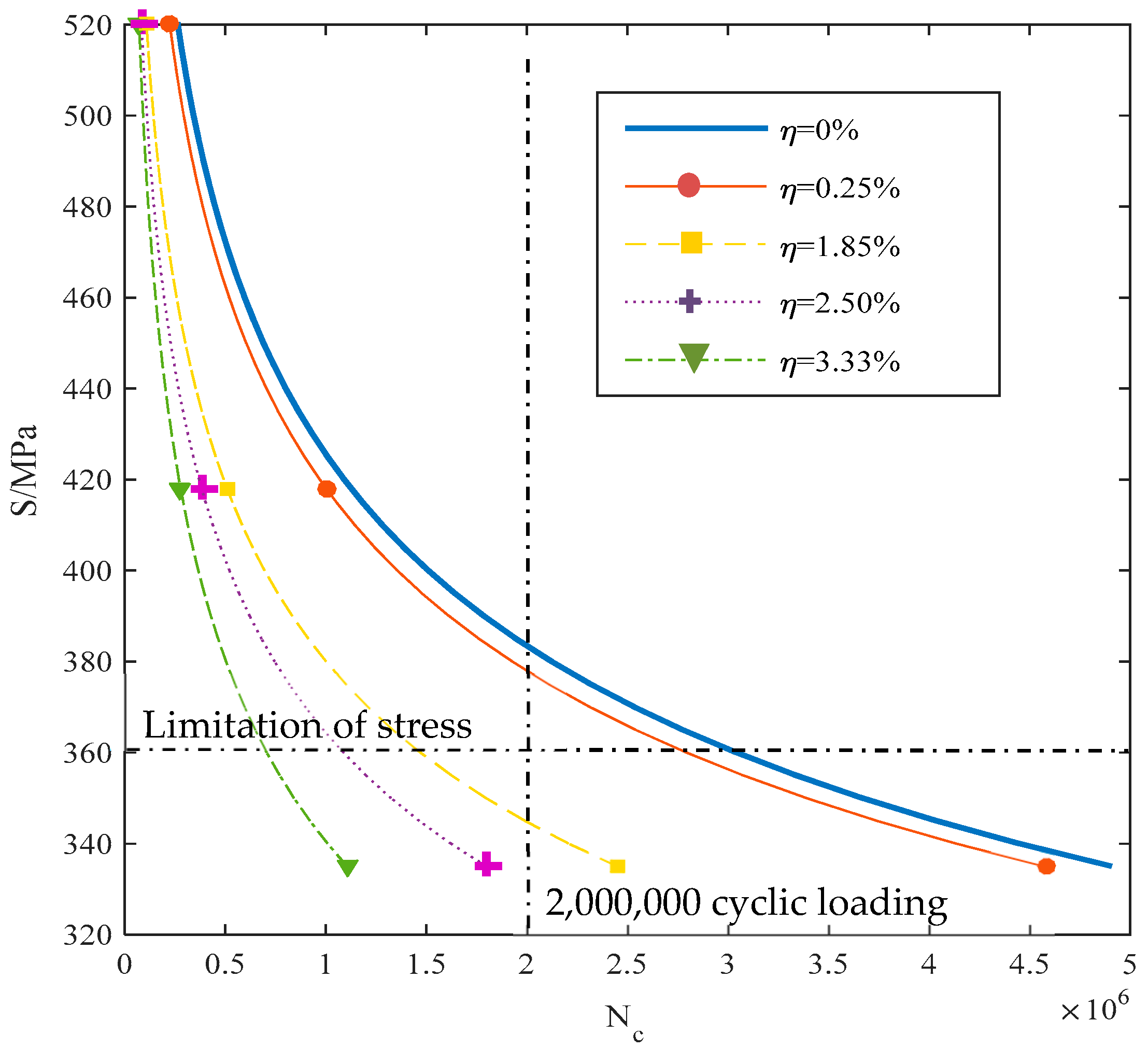
3.1. Fatigue Life of Pre-Corroded Steel Wire
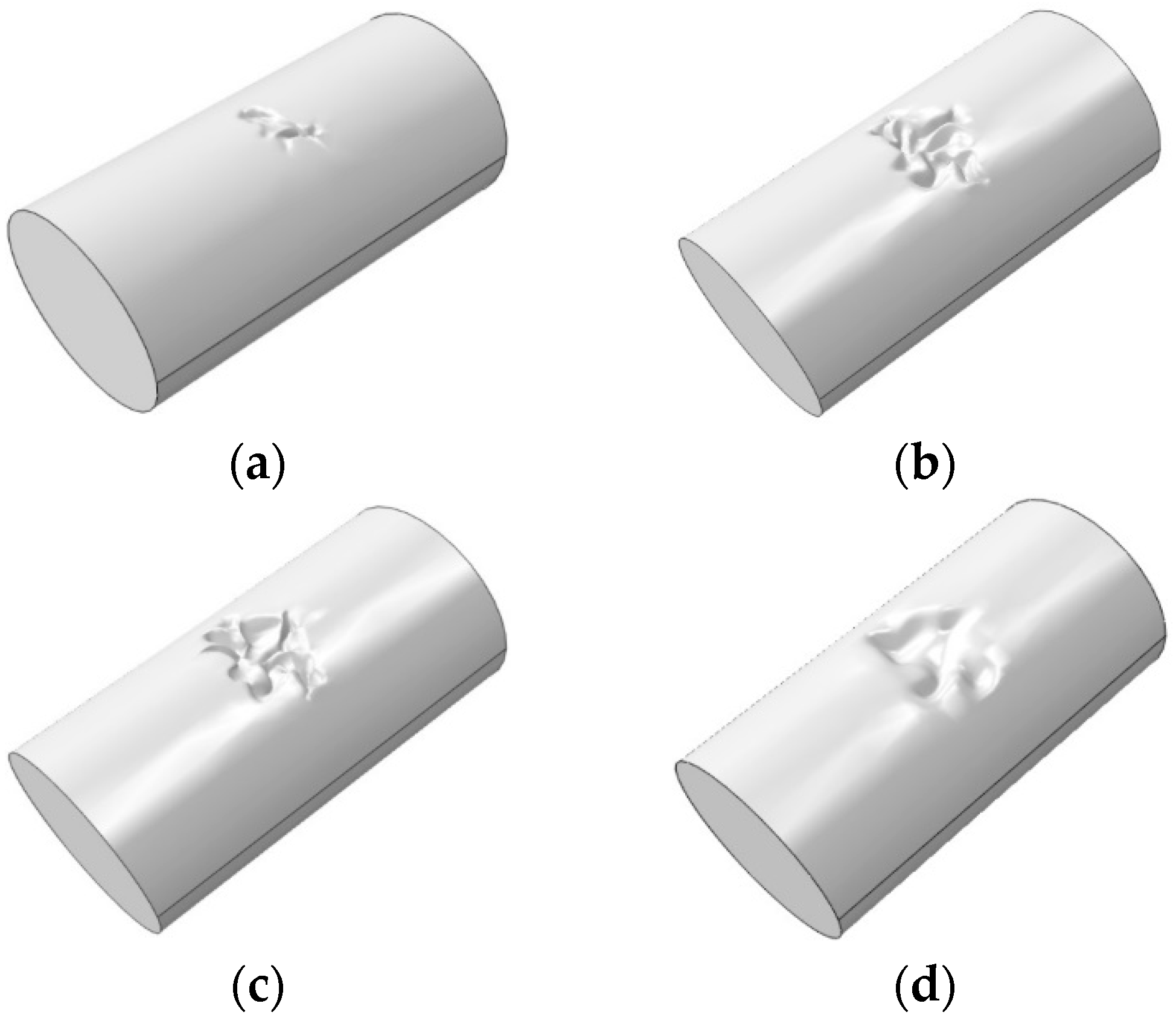
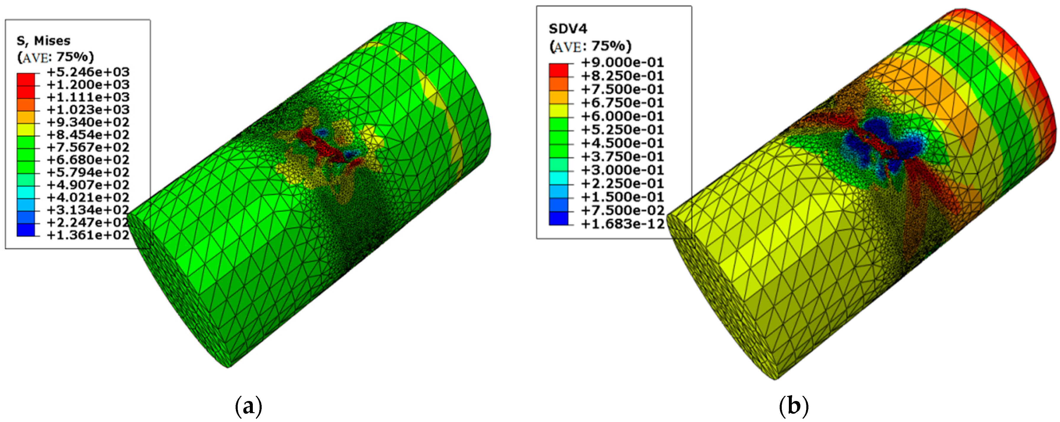
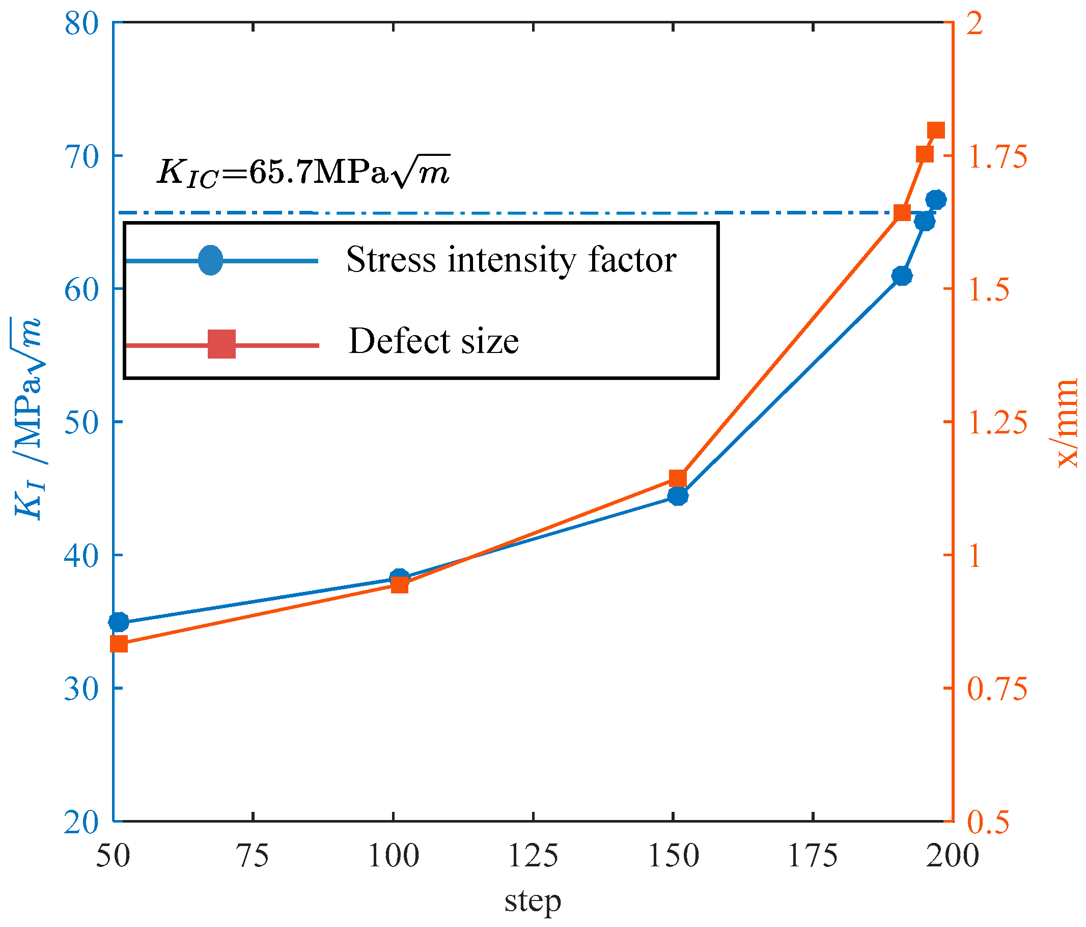
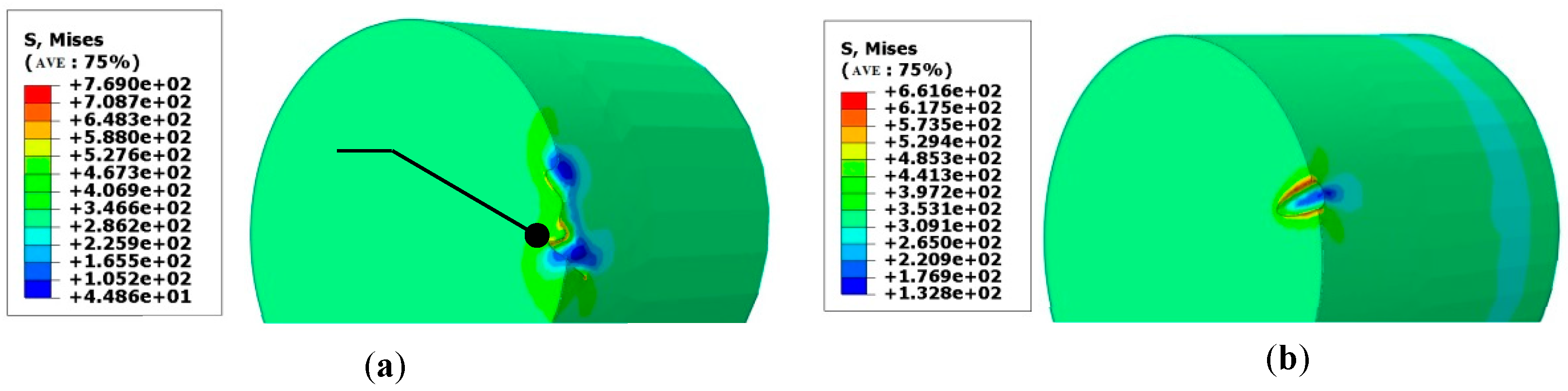
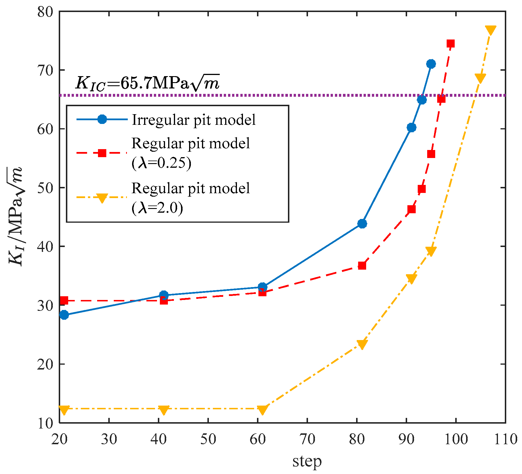
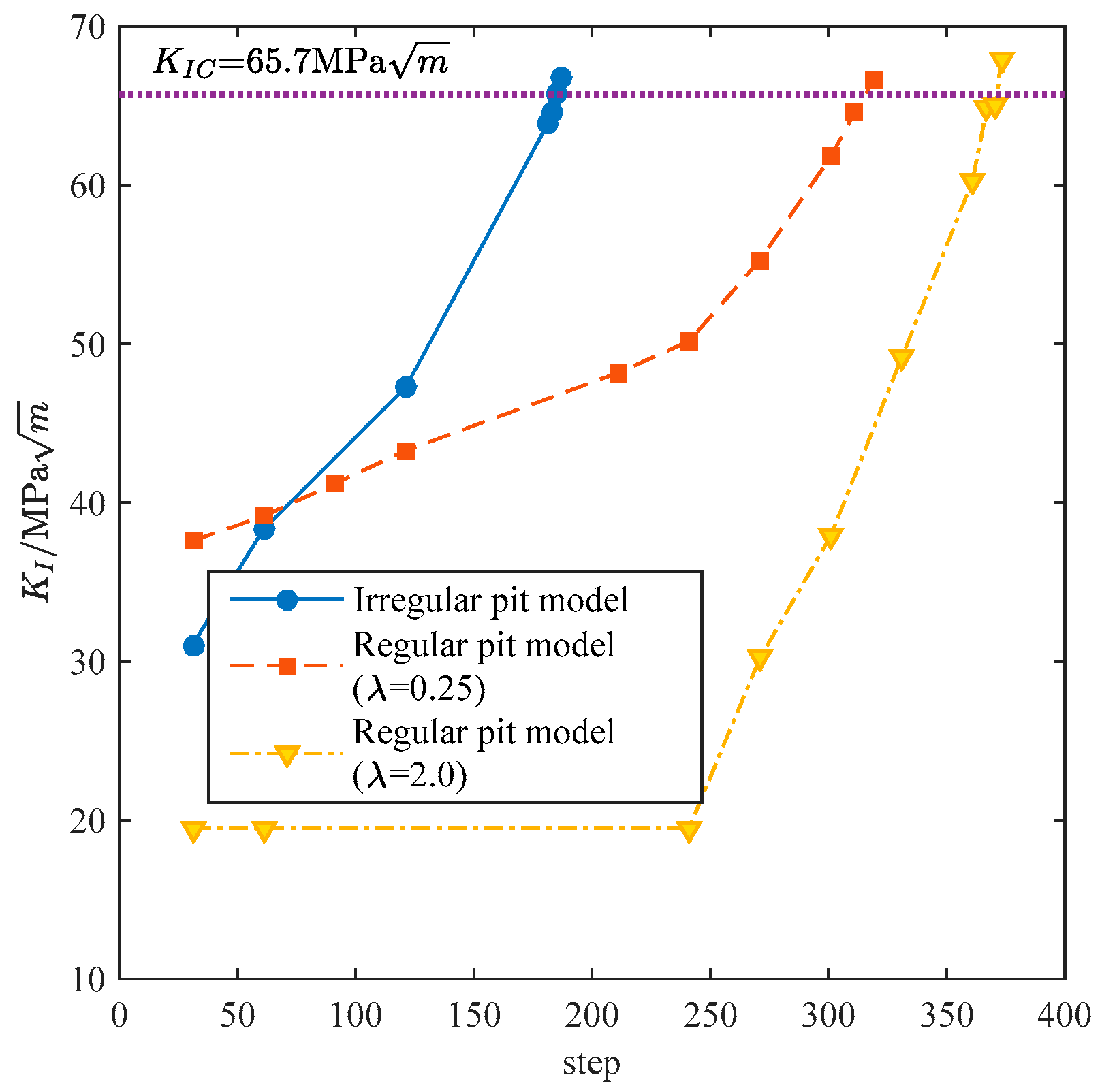
3.2. The Process of Damage Evolution
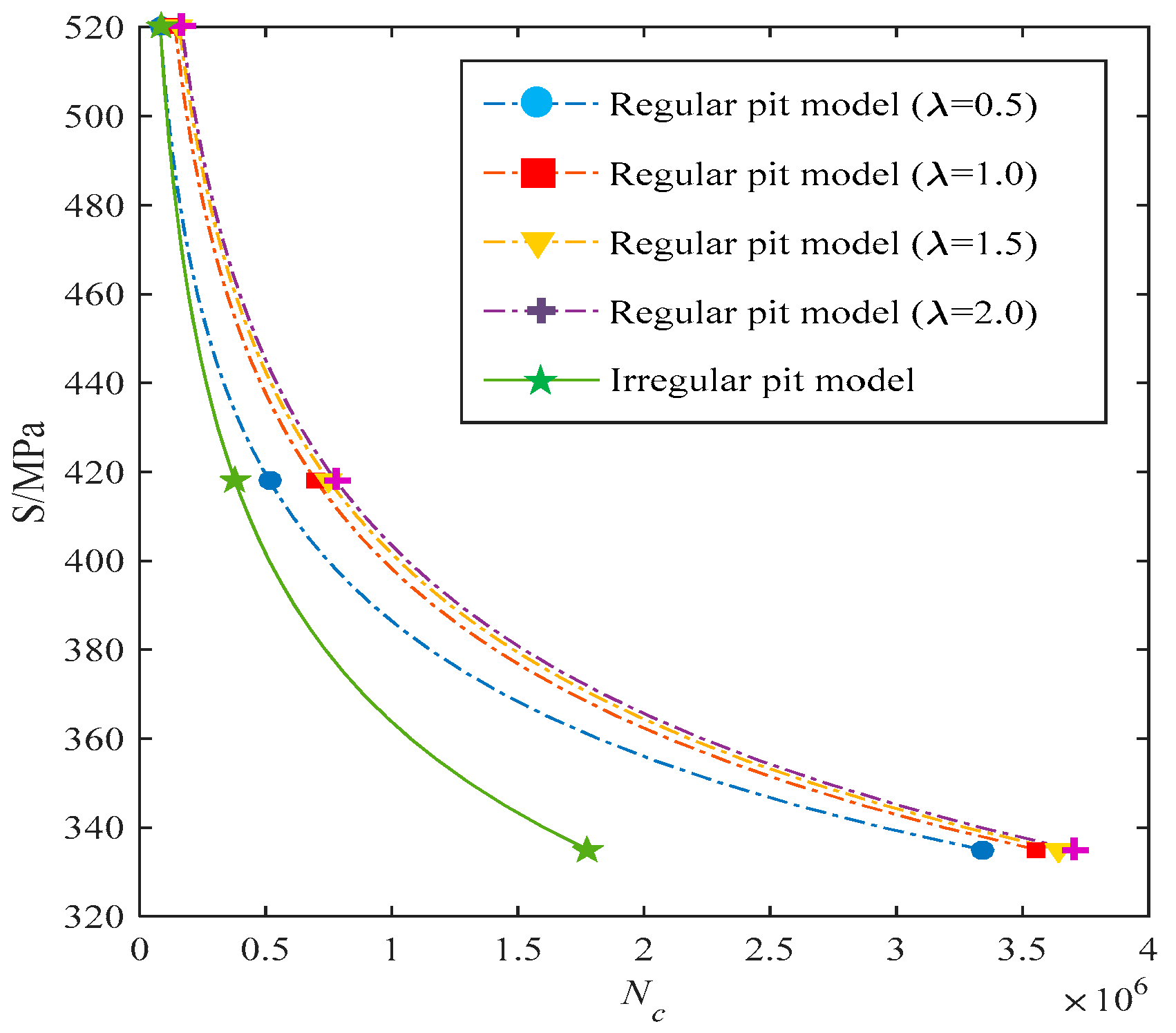
3.3. Influence of the Initial Pitting Morphology on the Fatigue Life
4. Conclusions
Author Contributions
Funding
Conflicts of Interest
References
- Watson, S.C.; Stafford, D. Cables in trouble. Civ. Eng. ASCE 1988, 58, 38–41. [Google Scholar]
- Dawson, D.B.; Pelloux, R.M. Corrosion fatigue crack growth of titanium alloys in aqueous environments. Metall. Trans. 1974, 5, 723–731. [Google Scholar] [CrossRef]
- Müller, M. Theoretical Considerations on Corrosion Fatigue Crack Initiation. Metall. Trans. A 1982, 13, 649–655. [Google Scholar] [CrossRef]
- Hirose, Y.; Mura, T. Crack nucleation and propagation of corrosion fatigue in high-strength steel. Eng. Fract. Mech. 1985, 22, 859–870. [Google Scholar] [CrossRef]
- Kim, S.; Kang, Y.J. Structural behavior of cable-stayed bridges after cable failure. Struct. Eng. Mech. 2016, 59, 1095–1120. [Google Scholar] [CrossRef]
- Mahmoud, K.M. Fracture strength for a high strength steel bridge cable wire with a surface crack. Theor. Appl. Fract. Mech. 2007, 48, 152–160. [Google Scholar] [CrossRef]
- Zheng, X.L.; Xie, X.; Li, X.Z.; Hu, J.M.; Sun, W.Z. Fatigue fracture surface analysis and fatigue life estimation of corroded steel wires. China J. Highw. Transp. 2017, 30, 79–86. (In Chinese) [Google Scholar]
- Sankaran, K.K.; Perez, R.; Jata, K.V. Effects of pitting corrosion on the fatigue behavior of aluminum alloy 7075-T6: Modeling and experimental studies. Mater. Sci. Eng. A (Struct. Mater. Prop. Microstruct. Process.) 2001, 297, 223–229. [Google Scholar] [CrossRef]
- Nakamura, S.I.; Suzumura, K. Hydrogen embrittlement and corrosion fatigue of corroded bridge wires. J. Constr. Steel Res. 2009, 65, 269–277. [Google Scholar] [CrossRef]
- Nakamura, S.; Suzumura, K. Experimental Study on Fatigue Strength of Corroded Bridge Wires. J. Bridge Eng. 2013, 18, 200–209. [Google Scholar] [CrossRef]
- Zheng, X.; Xie, X.; Li, X. Experimental Study and Residual Performance Evaluation of Corroded High-Tensile Steel Wires. J. Bridge Eng. 2017, 22, 04017091. [Google Scholar] [CrossRef]
- Chao, J.; Chong, W.; Xu, J. Experimental study on fatigue performance of corroded high-strength steel wires used in bridges. Constr. Build. Mater. 2018, 187, 681–690. [Google Scholar]
- Ye, H.W.; Huang, Y.; Wang, Y.Q.; Qiang, S.Z. Fatigue life estimation of corroded bridge wires based on theory of critical distances. J. Southwest Jiatong Univ. 2015, 50, 294–299. (In Chinese) [Google Scholar]
- Turnbull, A.; Wright, L.; Crocker, L. New insight into the pit-to-crack transition from finite element analysis of the stress and strain distribution around a corrosion pit. Corros. Sci. 2010, 52, 1492–1498. [Google Scholar] [CrossRef]
- Li, C.X.; Tang, X.S.; Xiang, G.B. Fatigue crack growth of cable steel wires in a suspension bridge: Multiscaling and mesoscopic fracture mechanics. Theor. Appl. Fract. Mech. 2010, 53, 113–126. [Google Scholar] [CrossRef]
- Sun, B. A continuum model for damage evolution simulation of the high strength bridge wires due to corrosion fatigue. J. Constr. Steel Res. 2018, 146, 76–83. [Google Scholar] [CrossRef]
- Hu, P.; Meng, Q.; Hu, W.; Shen, F.; Zhan, Z.; Sun, L. A continuum damage mechanics approach coupled with an improved pit evolution model for the corrosion fatigue of aluminum alloy. Corros. Sci. 2016, 113, 78–90. [Google Scholar] [CrossRef]
- GB/T18590-2001, Corrosion of Metals and Alloys-Evaluation of Pitting Corrosion; Standards Press of China: Beijing, China, 2001.
- Kachanov, L.M. Time rupture process under creep conditions. Izv. Akad. Nauk. Ssr 1958, 8, 26–31. [Google Scholar]
- Chowdhury, D.; Santen, L.; Schadschneider, A. Statistical physics of vehicular traffic and some related systems. Phys. Rep. 2000, 329, 199–329. [Google Scholar] [CrossRef] [Green Version]
- Wimpenny JW, T.; Colasanti, R. A unifying hypothesis for the structure of microbial biofilms based on cellular automaton models. Fems Microbiol. Ecol. 1997, 22, 1–16. [Google Scholar] [CrossRef]
- Ding, R.; Guo, Z.X. Microstructural modelling of dynamic recrystallisation using an extended cellular automaton approach. Comput. Mater. Sci. 2002, 23, 209–218. [Google Scholar] [CrossRef]
- di Caprio, D.; Vautrin-Ul, C.; Stafiej, J.; Saunier, J.; Chaussé, A.; Féron, D.; Badiali, J.P. Morphology of corroded surfaces: Contribution of cellular automaton modelling. Corros. Sci. 2011, 53, 418–425. [Google Scholar] [CrossRef]
- Caprio, D.D.; Vautrinul, C.; Stafiej, J.; Chausse, A.; Feron, D.; Badiali, P.J. Cellular automata approach for morphological evolution of localised corrosion. Br. Corros. J. 2013, 46, 223–227. [Google Scholar] [CrossRef]
- Stafiej, J.; Caprio, D.D.; Bartosik, U. Corrosion-passivation processes in a cellular automata based simulation study. J. Supercomput. 2013, 65, 697–709. [Google Scholar] [CrossRef] [Green Version]
- Leifer, J.; Mickalonis, J.I. Prediction of aluminum pitting in natural waters via artificial neural network analysis. Corrosion 2000, 56, 563–571. [Google Scholar] [CrossRef]
- Rajasankar, J.; Iyer, N.R. A probability-based model for growth of corrosion pits in aluminum alloys. Eng. Fract. Mech. 2006, 73, 553–570. [Google Scholar] [CrossRef]
- Rokhlin, S.I.; Kim, J.Y.; Nagy, H.; Zoofan, B. Effect of pitting corrosion on fatigue crack initiation and fatigue life. Eng. Fract. Mech. 1999, 62, 425–444. [Google Scholar] [CrossRef]
- Valor, A.; Caleyo, F.; Alfonso, L.; Rivas, D.; Hallen, J.M. Stochastic modeling of pitting corrosion: A new model for initiation and growth of multiple corrosion pits. Corros. Sci. 2007, 49, 559–579. [Google Scholar] [CrossRef]
- Wang, H.; Lu, G.; Wang, L.; Zhang, Y. Cellular automaton simulation of surface corrosion damage evolution. Acta Aeronaut. ET Astronaut. Sin. 2008, 30, 1490–1496. (In Chinese) [Google Scholar]
- Pidaparti, R.M.; Palakal, M.J.; Fang, L. Cellular Automation Approach to Model Aircraft Corrosion Pit Damage Growth. AIAA J. 2004, 42, 2562–2569. [Google Scholar] [CrossRef]
- Pidaparti, R.M.; Fang, L.; Palakal, M.J. Computational simulation of multi-pit corrosion process in materials. Comput. Mater. Sci. 2008, 41, 255–265. [Google Scholar] [CrossRef]
- Vautrin-Ul, C.; Taleb, A.; Stafiej, J.; Chausse, A.; Badiali, J.P. Mesoscopic modelling of corrosion phenomena: Coupling between electrochemical and mechanical processes, analysis of the deviation from the Faraday law. Electrochim. Acta 2007, 52, 5368–5376. [Google Scholar] [CrossRef]
- Lan, C.; Xu, Y.; Ren, D.L.; Li, N.; Liu, Z. Fatigue property assessment of parallel wire stay cable I: Fatigue life model for wire. China Civ. Eng. J. 2017, 50, 66–74. [Google Scholar]
- Zheng, X.L.; Xie, X.; Li, X.Z.; Tang, Z.Z. Fatigue crack propagation characteristics of high-tensile steel wires for bridge cables. Fatigue Fract. Eng. Mater. Struct. 2019, 42, 256–266. [Google Scholar] [CrossRef]
- Lan, C.; Xu, Y.; Liu, C.; Li, L.; Spencer, B.F., Jr. Fatigue life prediction for parallel-wire stay cables considering corrosion effects. Int. J. Fatigue 2018, 114, 81–91. [Google Scholar] [CrossRef]
- Wang, Y.; Zheng, Y.Q. Simulation of Damage Evolution and Study of Multi-fatigue Source Fracture of Steel Wire in Bridge Cables Under the Action of Pre-corrosion and Fatigue. CMES Comput. Model. Eng. Sci. 2019. [Google Scholar] [CrossRef]
- Pan, X.Y.; Xie, X.; Li, X.Z.; Sun, W.; Zhu, H.H. Mechanical properties and grading method of corroded high-tensile steel wires. J. Zhejiang Univ. (Eng. Sci.) 2014, 48, 1917–1924. [Google Scholar]
- GB/T 17101-2008, Hot-Dip Galvanized Wires for Bridge Cables; China Standard press: Beijing, China, 2008. (In Chinese)
- Harlow, D.G.; Wei, R.P. Probabilities of occurrence and detection of damage in airframe materials. Fatigue Fract. Eng. Mater. Struct. 2010, 22, 427–436. [Google Scholar] [CrossRef]
- Muhammet, C. Corrosion pit-induced stress concentration in spherical pressure vessel. Thin Walled Struct. 2019, 136, 106–112. [Google Scholar]


| η/% | S /MPa | n | Step | x/mm | Nc | Test Results of Fatigue Life [23] | Error | |
|---|---|---|---|---|---|---|---|---|
| 0.25% | 335 | 100,000 | 93 | 2.15662 | 64.9195 | 4,700,000 | 4,220,614 | 11.36% |
| 418 | 10,000 | 195 | 1.75383 | 64.9673 | 980,000 | 1,040,139 | 6.14% | |
| 520 | 10,000 | 45 | 1.34251 | 63.0924 | 230,000 | 240,066 | 4.19% | |
| 1.85% | 335 | 50,000 | 99 | 2.15101 | 64.7262 | 2,500,000 | 2,498,912 | 0.04% |
| 418 | 10,000 | 95 | 1.75383 | 64.9678 | 480,000 | 641,358 | 25.16% | |
| 520 | 2,000 | 109 | 1.9253 | 65.1381 | 110,000 | 173,800 | 36.71% | |
| 2.5% | 335 | 20,000 | 185 | 2.17891 | 65.6922 | 1,860,000 | 1,304,947 | 42.53% |
| 418 | 10,000 | 73 | 1.70954 | 63.3443 | 370,000 | 523,005 | 29.25% | |
| 520 | 1000 | 171 | 1.39672 | 65.3108 | 86,000 | 119,363 | 27.95% | |
| 3.33% | 335 | 10,000 | 189 | 2.15813 | 64.9717 | 950,000 | 821,534 | 15.64% |
| 418 | 10,000 | 73 | 1.71762 | 63.6386 | 370,000 | 398,024 | 7.04% | |
| 520 | 2000 | 61 | 1.40164 | 65.5137 | 61,000 | 96,681 | 36.90% |
| n | x/mm | |||
|---|---|---|---|---|
| 335 | 100,000 | 0.25 | 0.90246 | 4,900,000 |
| 0.5 | 0.5685 | 5,000,000 | ||
| 1.0 | 0.358 | 5,100,000 | ||
| 1.5 | 0.27331 | 5,200,000 | ||
| 2.0 | 0.2256 | 5,400,000 | ||
| 418 | 10,000 | 0.25 | 0.90246 | 1,060,000 |
| 0.5 | 0.5685 | 1,080,000 | ||
| 1.0 | 0.358 | 1,090,000 | ||
| 1.5 | 0.27331 | 1,100,000 | ||
| 2.0 | 0.2256 | 1,200,000 | ||
| 520 | 5000 | 0.25 | 0.90246 | 235,000 |
| 0.5 | 0.5685 | 245,000 | ||
| 1.0 | 0.358 | 250,000 | ||
| 1.5 | 0.27331 | 255,000 | ||
| 2.0 | 0.2256 | 280,000 |
| n | x/mm | |||
|---|---|---|---|---|
| 335 | 20,000 | 0.25 | 1.9443 | 2,100,000 |
| 0.5 | 1.2248 | 3,180,000 | ||
| 1.0 | 0.7716 | 3,560,000 | ||
| 1.5 | 0.589 | 3,640,000 | ||
| 2.0 | 0.486 | 3,720,000 | ||
| 418 | 10,000 | 0.25 | 1.9443 | - |
| 0.5 | 1.2248 | 600,000 | ||
| 1.0 | 0.7716 | 730,000 | ||
| 1.5 | 0.589 | 790,000 | ||
| 2.0 | 0.486 | 800,000 | ||
| 520 | 1000 | 0.25 | 1.9443 | - |
| 0.5 | 1.2248 | 78,000 | ||
| 1.0 | 0.7716 | 141,000 | ||
| 1.5 | 0.589 | 158,000 | ||
| 2.0 | 0.486 | 168,000 |
© 2019 by the authors. Licensee MDPI, Basel, Switzerland. This article is an open access article distributed under the terms and conditions of the Creative Commons Attribution (CC BY) license (http://creativecommons.org/licenses/by/4.0/).
Share and Cite
Wang, Y.; Zheng, Y. Research on the Damage Evolution Process of Steel Wire with Pre-Corroded Defects in Cable-Stayed Bridges. Appl. Sci. 2019, 9, 3113. https://doi.org/10.3390/app9153113
Wang Y, Zheng Y. Research on the Damage Evolution Process of Steel Wire with Pre-Corroded Defects in Cable-Stayed Bridges. Applied Sciences. 2019; 9(15):3113. https://doi.org/10.3390/app9153113
Chicago/Turabian StyleWang, Ying, and Yuqian Zheng. 2019. "Research on the Damage Evolution Process of Steel Wire with Pre-Corroded Defects in Cable-Stayed Bridges" Applied Sciences 9, no. 15: 3113. https://doi.org/10.3390/app9153113
APA StyleWang, Y., & Zheng, Y. (2019). Research on the Damage Evolution Process of Steel Wire with Pre-Corroded Defects in Cable-Stayed Bridges. Applied Sciences, 9(15), 3113. https://doi.org/10.3390/app9153113