Transverse Vibration of Clamped-Pinned-Free Beam with Mass at Free End

Abstract

Engineering systems undergoing extreme and harsh environments can often times experience rapid damaging effects. In order to minimize loss of economic investment and human lives, structural health monitoring (SHM) of these high-rate systems is being researched. An experimental testbed has been developed to validate SHM methods in a controllable and repeatable laboratory environment. This study applies the Euler-Bernoulli beam theory to this testbed to develop analytical solutions of the system. The transverse vibration of a clamped-pinned-free beam with a point mass at the free end is discussed in detail. Results are derived for varying pin locations and mass values. Eigenvalue plots of the first five modes are presented along with their respective mode shapes. The theoretical calculations are experimentally validated and discussed.

1. Introduction

High-rate dynamics are defined as events having amplitudes greater than 100 g over durations less than 100 ms [1]. Some examples of high-rate systems may include civil structures exposed to blast, passenger vehicles experiencing collisions, and aerial or spacecraft vehicles subjected to ballistic impacts. Such systems have the potential to experience rapid changes in mechanical configuration through damage. Economic investments and lives could be saved if fast detection of parameter changes can be accurately quantified [2]. A variable input observer has been studied by the authors as a potential solution to increasing convergence times through richer inputs [3]. However, there is a need to validate high-rate structural health monitoring (SHM) methods [4].

An experimental testbed has been designed and built to test and validate SHM methods systems experiencing high-rate dynamics. The development of an experimental testbed is critical, because the experimentation on real-life high-rate systems would be complex, difficulty to verify, and potentially very costly. This testbed design incorporates a cantilever beam with a roller that restrains the displacement in the vertical direction and is allowed to move freely along the length of the beam. Additionally, the mass at the free end of the beam can be dropped through the de-energizing of the electromagnet that detaches the mass from the beam. The roller is a moving cart that provides a changing boundary condition while the mass drop provides a sudden change in mechanical configuration. This system is easily controllable and repeatable in a laboratory setting.

To develop analytical solutions for this beam structure, the Euler-Bernoulli beam theory is applied. The system is modeled as clamped-pinned-free with a point mass at free end. To the best knowledge of the authors, this configuration has not been previously studied analytically nor experimentally. There is no mention of this beam configuration in the book authored by Blevins [5]. The clamped-pinned-free without mass [6] and the clamped-free with mass at free end without pin [7] have been studied. In more recent years, researchers have investigated the free vibration of multi-span beams with flexible constraints [8], axial vibrations of multi-span beams with concentrated masses [9], multi-span beams with moving masses [10], and multi-span beams carrying spring-mass systems [11,12].

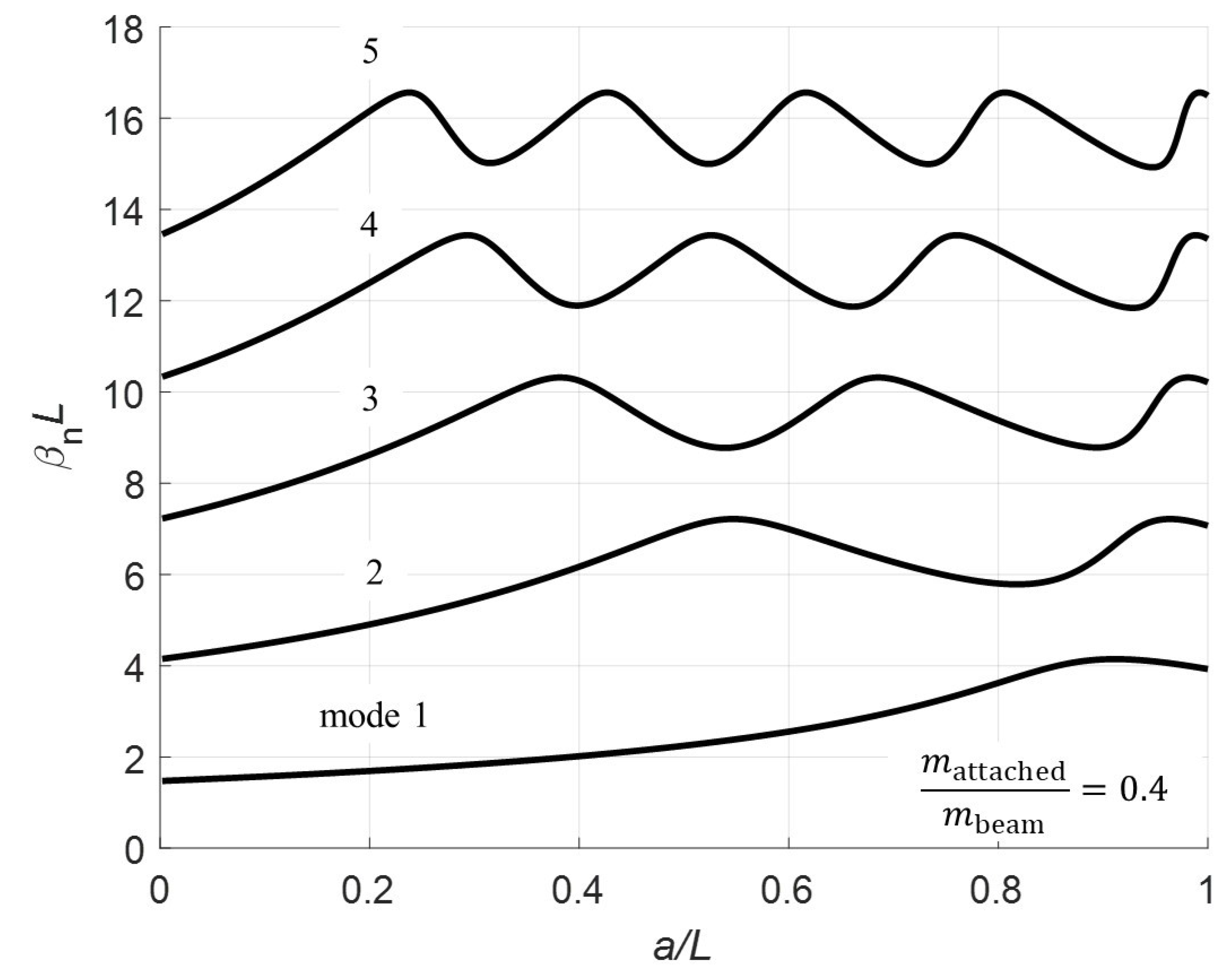
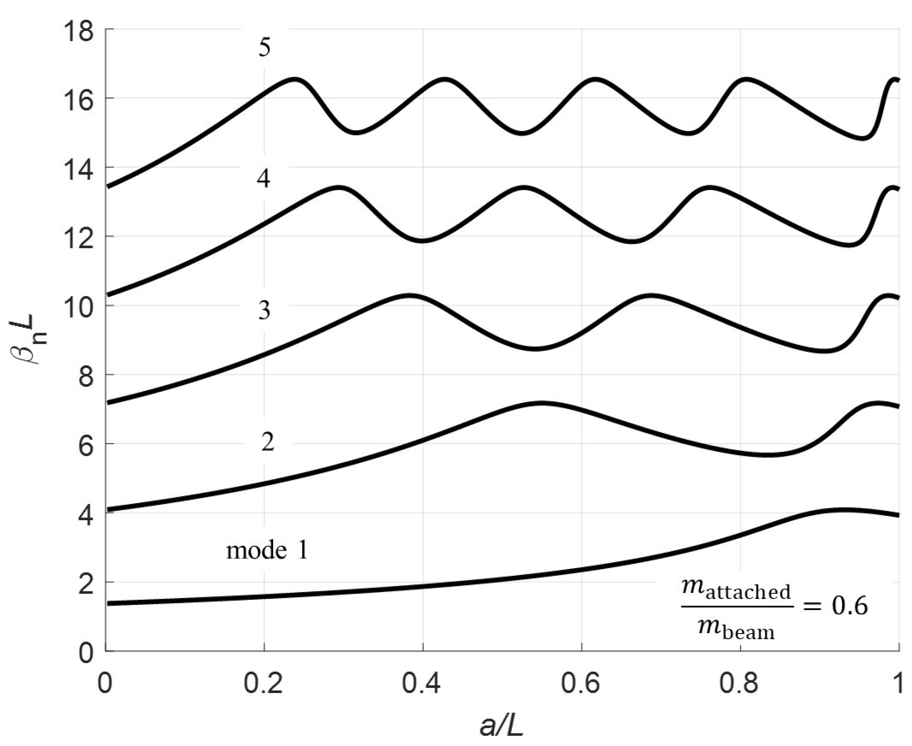
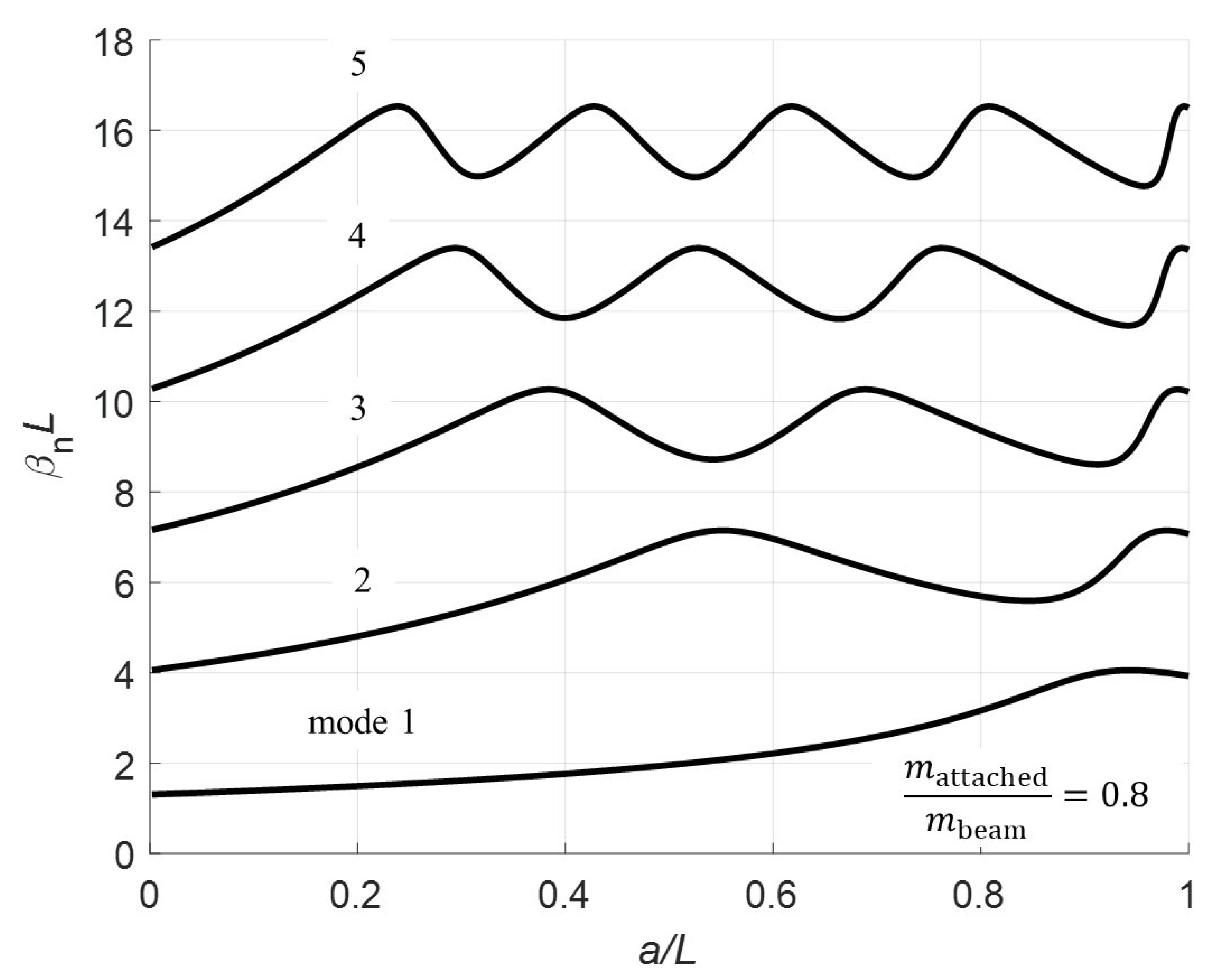
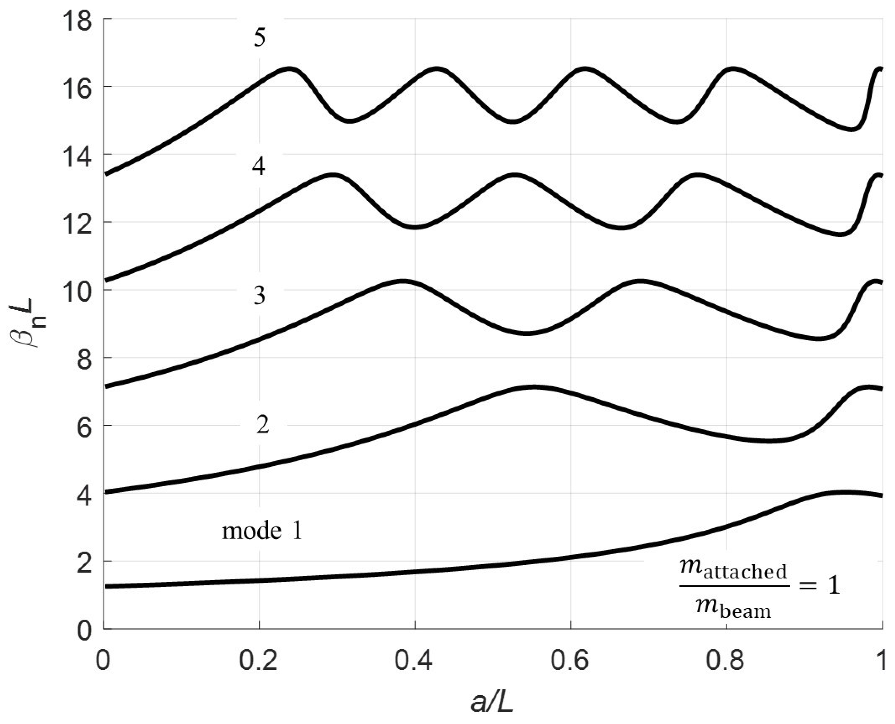
Using beam theory, Section 2 derives the transcendental equation. A generalized form is presented that is applicable to any pin location and any mass value. Derived results are verified through comparison between well known cases in literature. Section 3 calculates the eigenvalues for normalized pinned location for various mass ratios. Section 4 calculates the mode shapes for several different pinned locations, while Section 5 compares the results from the theoretical calculations to experimental data.

2. Frequency Calculations

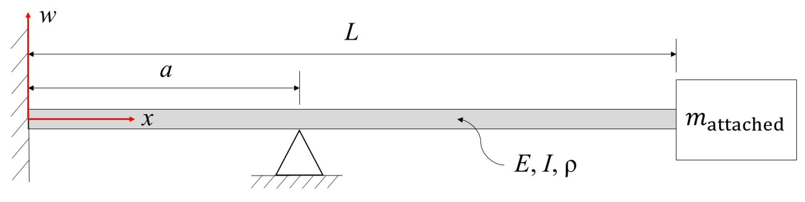
The transverse vibrations of a slender clamped-pinned-free beam with a mass at free end of interest is shown in Figure 1. The governing equation for the beam using Euler-Bernoulli’s beam theory [13] can be written:

$$\rho A\frac{{\partial }^{2}w}{\partial t^2}+EI\frac{{\partial }^{4}w}{\partial x^4}=0$$

(1)

where E is the Young’s modulus, I is the cross-sectional moment of inertia, w is the vertical deflection, x is the axial coordinate, $\rho$ is the density of the beam, A is the cross-sectional area, and t is time. Equation (1) can be solved assuming a separation-of-variables solution in the standard form:

$$w(x,t)=X(x)T(t)$$

(2)

where X is the spatial solution and T is the temporal solution. The spatial solution for a two-span beam then is expressed:

$$X(x)=\left\{\begin{array}{cc}{X}_1(x),\hfill & 0\le x\le a\hfill \\ X_2(x),\hfill & a\le x\le L\hfill \end{array}\right.$$

(3)

The sub-functions in Equation (3) can be written as the following general solutions:

$$\begin{array}{cc}\hfill X_1(x)& =a_{1}sin(\beta x)+a_{2}cos(\beta x)+a_{3}sinh(\beta x)+a_{4}cosh(\beta x)\hfill \end{array}$$

(4)

$$\begin{array}{cc}\hfill X_2(x)& =b_{1}sin(\beta x)+b_{2}cos(\beta x)+b_{3}sinh(\beta x)+b_{4}cosh(\beta x)\hfill \end{array}$$

(5)

where $\beta$ is the beam vibration eigenvalue. Parameter $\beta$ and seven of the eight coefficients can be solved by applying the boundary conditions of the system. For the clamped-pinned-free, the displacement and slope at the clamped end are zero [7]:

$$\begin{array}{c}{X}_1(0)=0\end{array}$$

(6)

$$\begin{array}{c}\frac{d{X}_1(0)}{dx}=0\end{array}$$

(7)

while at the free end, the bending moment and the shear vanish such that:

$$\begin{array}{c}\frac{d^2{X}_2(L)}{d{x}^2}=0\end{array}$$

(8)

$$\begin{array}{c}EI\frac{d^3{X}_2(L)}{d{x}^3}=m_{\mathrm{attached}}\frac{d^2{T}_2(L,t)}{d{t}^2}\end{array}$$

(9)

where $m_{\mathrm{attached}}$ is the mass attached to the beam at the free end. In addition to these four boundary conditions, four more boundary conditions (displacement and rotation) are found at the pin location a:

$$\begin{array}{c}{X}_1(a)=0\end{array}$$

(10)

$$\begin{array}{c}{X}_2(a)=0\end{array}$$

(11)

$$\begin{array}{c}\frac{d{X}_1(a)}{dx}=\frac{d{X}_2(a)}{dx}\end{array}$$

(12)

$$\begin{array}{c}\frac{d^2{X}_1(a)}{d{x}^2}=\frac{d^2{X}_2(a)}{d{x}^2}\end{array}$$

(13)

Substituting the first transverse displacement (Equation (4)) into the clamped boundary condition (Equations (6) and (7)) gives:

$$\begin{array}{c}{a}_2+a_4=0\end{array}$$

(14)

$$\begin{array}{c}{a}_1+a_3=0\end{array}$$

(15)

Substituting the second transverse displacement (Equation (5)) into the free end boundary condition (Equation (8)) yields:

$$-b_{1}sin(\beta L)-b_{2}cos(\beta L)+b_{3}sinh(\beta L)+b_{4}cosh(\beta L)=0$$

(16)

Additionally, inserting the second transverse displacement (Equation (5)) into Equation (1) and applying the boundary condition at the free end (Equation (9)) results in:

$$\begin{array}{c}{b}_1(-cos(\beta L)+\beta L\frac{m_{\mathrm{attached}}}{m_{\mathrm{beam}}}sin(\beta L))+b_2(sin(\beta L)+\beta L\frac{m_{\mathrm{attached}}}{m_{\mathrm{beam}}}cos(\beta L))\\ +b_3(cosh(\beta L)+\beta L\frac{m_{\mathrm{attached}}}{m_{\mathrm{beam}}}sinh(\beta L))+b_4(sinh(\beta L)+\beta L\frac{m_{\mathrm{attached}}}{m_{\mathrm{beam}}}cosh(\beta L))=0\end{array}$$

(17)

where $m_{\mathrm{beam}}$ is the mass of the beam.

Substituting the first transverse displacement (Equation (4)) into the pinned boundary condition (Equations (10) and (11)) results in:

$$\begin{array}{c}{a}_{1}sin(\beta L\frac{a}{L})+a_{2}cos(\beta L\frac{a}{L})+a_{3}sinh(\beta L\frac{a}{L})+a_{4}cosh(\beta L\frac{a}{L})=0\end{array}$$

(18)

and

$$\begin{array}{c}{b}_{1}sin(\beta L\frac{a}{L})+b_{2}cos(\beta L\frac{a}{L})+b_{3}sinh(\beta L\frac{a}{L})+b_{4}cosh(\beta L\frac{a}{L})=0\end{array}$$

(19)

After, substituting the second transverse displacement (Equation (5)) into the boundary conditions defined by Equations (12) and (13) provides the following expressions:

$$\begin{array}{c}{a}_{1}cos(\beta L\frac{a}{L})-a_{2}sin(\beta L\frac{a}{L})+a_{3}cosh(\beta L\frac{a}{L})+a_{4}sinh(\beta L\frac{a}{L})\\ -b_{1}cos(\beta L\frac{a}{L})+b_{2}sin(\beta L\frac{a}{L})-b_{3}cosh(\beta L\frac{a}{L})-b_{4}sinh(\beta L\frac{a}{L})=0\end{array}$$

(20)

$$\begin{array}{c}-a_{1}sin(\beta L\frac{a}{L})-a_{2}cos(\beta L\frac{a}{L})+a_{3}sinh(\beta L\frac{a}{L})+a_{4}cosh(\beta L\frac{a}{L})\\ +b_{1}sin(\beta L\frac{a}{L})+b_{2}cos(\beta L\frac{a}{L})-b_{3}sinh(\beta L\frac{a}{L})-b_{4}cosh(\beta L\frac{a}{L})=0\end{array}$$

(21)

Aggregating Equations (14)–(21) into an $8\times 8$ matrix (see Appendix A) and solving for the determinant leads to the transcendental equation expressed:

$$\begin{array}{c}4cos(\beta L(\frac{a}{L}-1))sinh(\beta L(\frac{a}{L}-1))-4cosh(\beta L(\frac{a}{L}-1))sin(\beta L(\frac{a}{L}-1))\\ +2cos(\beta L(2\frac{a}{L}-1))sinh(\beta L)-2cosh(\beta L(2\frac{a}{L}-1))sin(\beta L)\\ +4cos(\frac{a}{L}\beta L)sinh(\frac{a}{L}\beta L)-4cosh(\frac{a}{L}\beta L)sin(\frac{a}{L}\beta L)\\ +2cos(\beta L)sinh(\beta L)-2cosh(\beta L)sin(\beta L)+8\beta L\frac{m_{\mathrm{attached}}}{m_{\mathrm{beam}}}sin(\beta L(\frac{a}{L}-1))sinh(\beta L(\frac{a}{L}-1))\\ +2\beta L\frac{m_{\mathrm{attached}}}{m_{\mathrm{beam}}}cos(\beta L(2\frac{a}{L}-1))cosh(\beta L)-2\beta L\frac{m_{\mathrm{attached}}}{m_{\mathrm{beam}}}cosh(\beta L(2\frac{a}{L}-1))cos(\beta L)\\ +2\beta L\frac{m_{\mathrm{attached}}}{m_{\mathrm{beam}}}sin(\beta L(2\frac{a}{L}-1))sinh(\beta L)+2\beta L\frac{m_{\mathrm{attached}}}{m_{\mathrm{beam}}}sinh(\beta L(2\frac{a}{L}-1))sin(\beta L)\\ -4\beta L\frac{m_{\mathrm{attached}}}{m_{\mathrm{beam}}}sin(\beta L)sinh(\beta L)=0\end{array}$$

(22)

where the natural frequencies (in Hz) are given by:

$$f_n=\frac{{({\beta }_{n}L)}^2}{2\pi L^2}\sqrt{\frac{EI}{\rho A}}$$

(23)

To verify Equation (22), the first five natural frequencies were calculated for three well known cases:

• Case 1: Clamped-free [14]: $\frac{a}{L}=\frac{m_{\mathrm{attached}}}{m_{\mathrm{beam}}}=0$
• Case 2: Clamped-free with mass at free end [7]: $\frac{a}{L}=0$
• Case 3: Clamped-pinned-free [6]: $\frac{m_{\mathrm{attached}}}{m_{\mathrm{beam}}}=0$

The results are tabulated in

Table 1. Comparison of analytical results: clamped-free (Case 1).

	Literature [14]	Proposed Model	Difference
Mode	(Hz)	(Hz)	(%)
1	19.64	19.63	0.051
2	123.07	123.02	0.041
3	344.64	344.45	0.055
4	675.31	674.97	0.050
5	1116.33	1115.79	0.048

,

Table 2. Comparison of analytical results: Clamped-free with mass at free end ($\frac{m_{\mathrm{attached}}}{m_{\mathrm{beam}}}=0.2$) (Case 2).

	Literature [7]	Proposed Model	Difference
Mode	(Hz)	(Hz)	(%)
1	14.56	14.58	0.14
2	101.47	101.64	0.17
3	298.59	299.00	0.14
4	603.06	604.02	0.16
5	1017.07	1018.48	0.14

and

Table 3. Comparison of analytical results: Clamped-pinned-free (pinned at $a=200$ mm) (Case 3).

	Literature [6]	Proposed Model	Difference
Mode	(Hz)	(Hz)	(%)
1	41.70	41.59	0.26
2	279.25	278.46	0.28
3	635.80	635.19	0.10
4	899.94	897.69	0.25
5	1650.85	1646.48	0.26

. The frequencies of the first five modes (${\beta }_1$–${\beta }_5$) are compared between what is found in literature against the results from Equation (22) (proposed model). The small differences are due to rounding errors of the beam vibration eigenvalues $\beta$, which cause large changes in the calculated frequency ($f_n\propto {\beta }_n^2$). The precision for $\beta$ in this paper is $\pm 0.0002$.

3. Calculations of Eigenvalues

The beam vibration eigenvalues are calculated in terms of $\beta L$ for different mass ratios, $\frac{m_{\mathrm{attached}}}{m_{\mathrm{beam}}}$. The eigenvalues are plotted as a function of the normalized pinned location, $\frac{a}{L}$ in Figure 2, Figure 3, Figure 4, Figure 5 and Figure 6. Note, the $\beta L$ values corresponding to $\frac{a}{L}=0$ is equivalent to the clamped-free system with a mass at the free.

4. Mode Shapes

The mode shapes are calculated for the two different sections of the beam corresponding to the clamped-pinned and pinned-free sections. To calculate the mode shapes, the boundary condition (Equations (6)–(13)) are used to find a relationship between the coefficients. The method used here consists of solving all coefficients in terms of $a_4$. Note, there are not enough equations to determine a unique solution for each coefficient. The solutions for the a coefficients are:

$$\begin{array}{c}{a}_1=-a_3\end{array}$$

(24)

$$\begin{array}{c}{a}_2=-a_4\end{array}$$

(25)

$$\begin{array}{c}{a}_3=\frac{cos(\beta L\frac{a}{L})-cosh(\beta L\frac{a}{L})}{(sinh(\beta L\frac{a}{L})-sin(\beta L\frac{a}{L})}{a}_4\end{array}$$

(26)

and for the b coefficients:

$$\begin{array}{c}{b}_1=-b_{2}cot(\beta L)+b_3\frac{sinh(\beta L)}{sin(\beta L)}+b_4\frac{cosh(\beta L)}{sin(\beta L)}\end{array}$$

(27)

$$\begin{array}{c}{b}_2=b_3\frac{z_1}{z_3}+b_4\frac{z_2}{z_3}\end{array}$$

(28)

$$\begin{array}{c}{b}_3=\frac{\frac{z_2{z}_4}{z_3}+z_6}{\frac{z_1{z}_4}{z_3}+z_5}\end{array}$$

(29)

where

$$\begin{array}{c}{z}_1=\frac{sinh(\beta L)}{sin(\beta L)}(cos(\beta L)+\beta L\frac{m_{\mathrm{attached}}}{m_{\mathrm{beam}}}sin(\beta L))-(cosh(\beta L)+\beta L\frac{m_{\mathrm{attached}}}{m_{\mathrm{beam}}}sinh(\beta L))\end{array}$$

(30)

$$\begin{array}{c}{z}_2=\frac{cosh(\beta L)}{sin(\beta L)}(cos(\beta L)+\beta L\frac{m_{\mathrm{attached}}}{m_{\mathrm{beam}}}sin(\beta L))-(sinh(\beta L)+\beta L\frac{m_{\mathrm{attached}}}{m_{\mathrm{beam}}}cosh(\beta L))\end{array}$$

(31)

$$\begin{array}{c}{z}_3=cot(\beta L)(cos(\beta L)+\beta L\frac{m_{\mathrm{attached}}}{m_{\mathrm{beam}}}sin(\beta L))+(sin(\beta L)+\beta L\frac{m_{\mathrm{attached}}}{m_{\mathrm{beam}}}cos(\beta L))\end{array}$$

(32)

$$\begin{array}{c}{z}_4=cos(\beta L\frac{a}{L})-cot(\beta L)sin(\beta L\frac{a}{L})\end{array}$$

(33)

$$\begin{array}{c}{z}_5=\frac{sinh(\beta L)}{sin(\beta L)}sin(\beta L\frac{a}{L})+sinh(\beta L\frac{a}{L})\end{array}$$

(34)

$$\begin{array}{c}{z}_6=\frac{cosh(\beta L)}{sin(\beta L)}sin(\beta L\frac{a}{L})+cosh(\beta L\frac{a}{L})\end{array}$$

(35)

Substituting the equations for the coefficients (Equations (24)–(35)) into the boundary condition from Equation (12), a relationship between $a_4$ and $b_4$ is obtained. For brevity, this expression is not presented here. The mode shapes are determined for the multi-span beam by substituting all coefficient expressions in terms of $a_4$ into Equation (3).

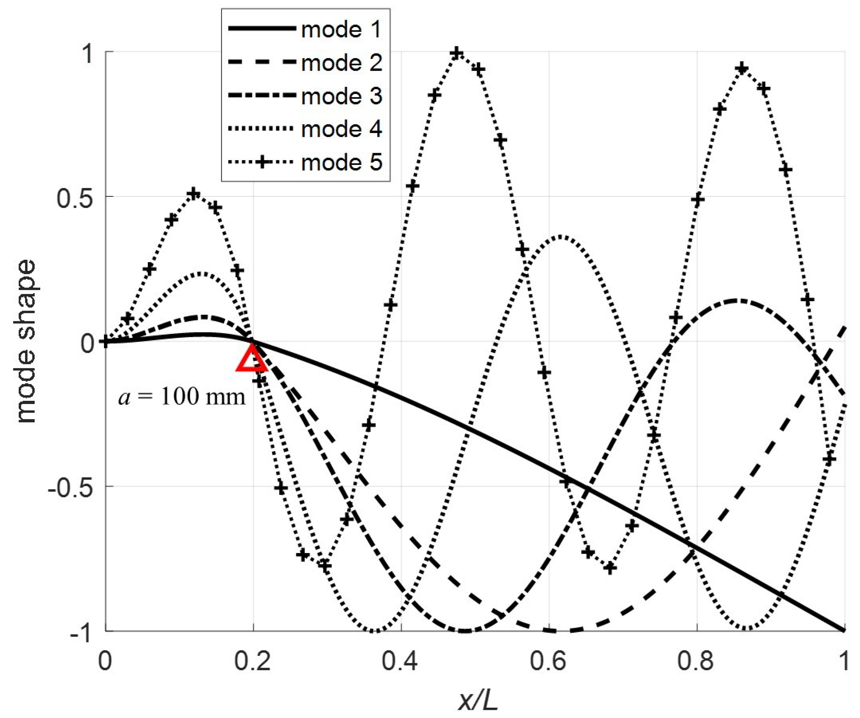
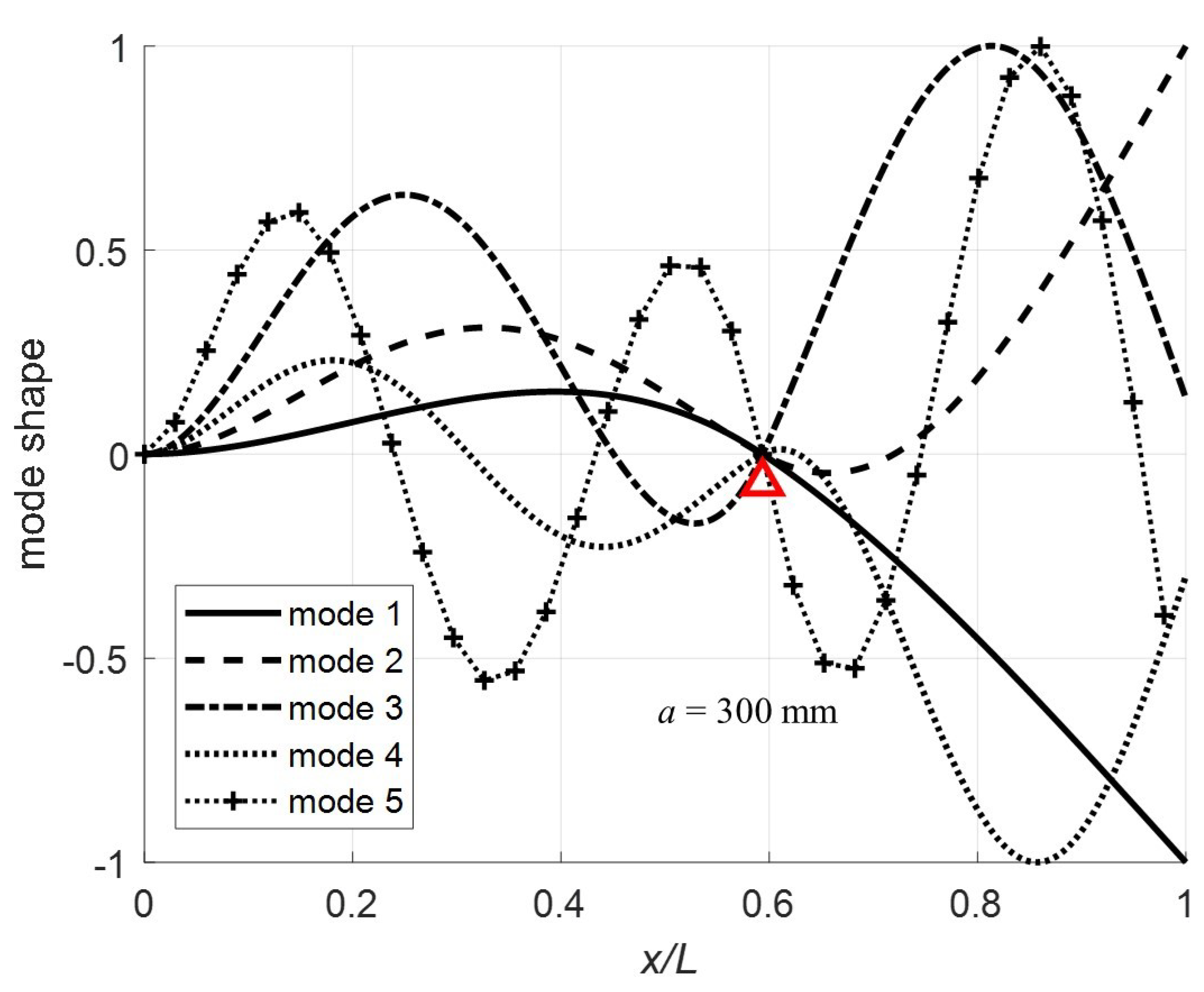
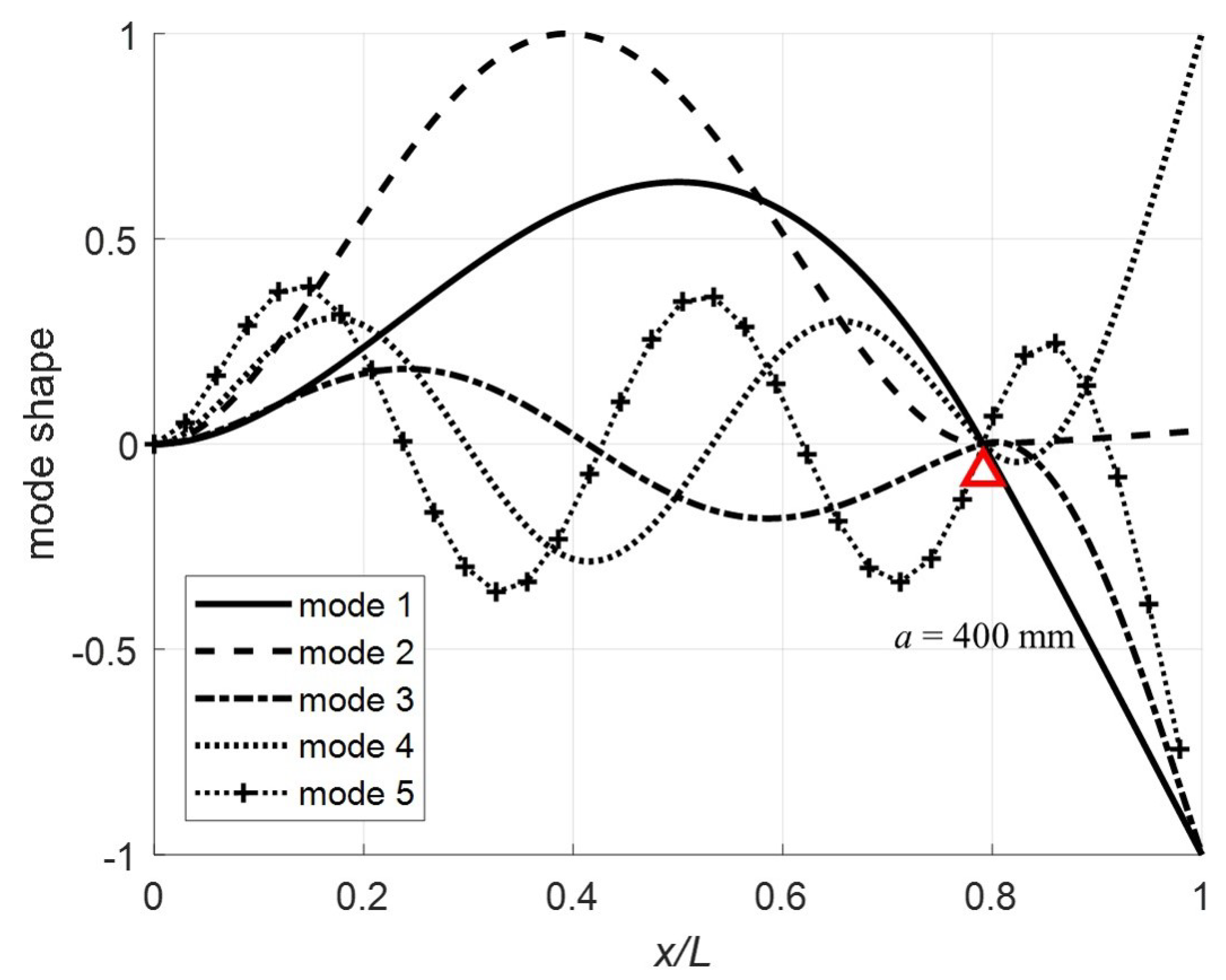
Normalizing at $a_4=1$, the first five mode shapes for the clamped-pinned-free beam with a mass at the free end are plotted in Figure 7, Figure 8, Figure 9 and Figure 10 for a = 100, 200, 300, and 400 mm with $\frac{m_{\mathrm{attached}}}{m_{\mathrm{beam}}}=0.2$. The red triangle on the plots denotes the pin location. Note that for $a=100$ (Figure 7), the mode shapes are as expected for a fixed-pinned-free cantilever beam with a mass on the free end. However, when $a=200$ (Figure 8), mode shape 4 is highly non-symmetric because the constraint point (pin) is just past the node and in combination with the effect of the mass this mode shape flattens out for the remainder of the beam. For $a=300$ (Figure 9) and $a=400$ (Figure 10) the more expected sinusoidal shape dominates the mode shapes.

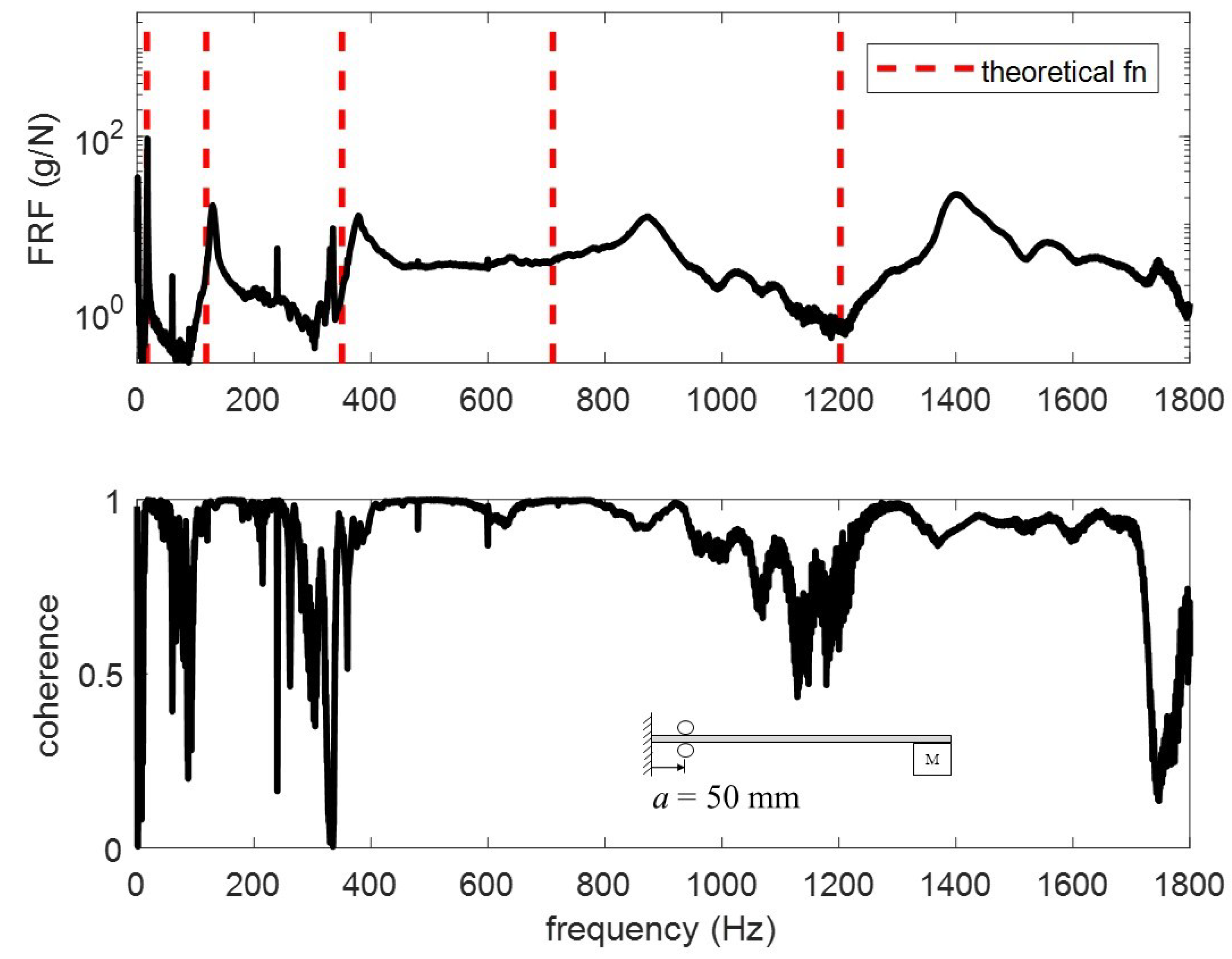
5. Experimental Validation

In this section, the theoretical results are compared with experimental data. The experimental setup is illustrated in Figure 11. A cart with rollers is used as a moving pin along the beam. Accelerometers are attached at locations 300 mm and 400 mm. The mass of the accelerometers is assumed to have a negligible effect. Each accelerometer weighs 1.7 gm, not including cables, which is 0.2% of the weight of the beam. At the free end, an electromagnet is used to simulate the point mass. The specifications of the experiment are listed in

Table 4. Specifications of the experimental setup.

Parameter	Value
L	505 mm
base	50 mm
height	6.4 mm
$\rho$	7970 kg/m${}^3$
E	190 GPa
$m_{\mathrm{attached}}$	0.259 Kg

.

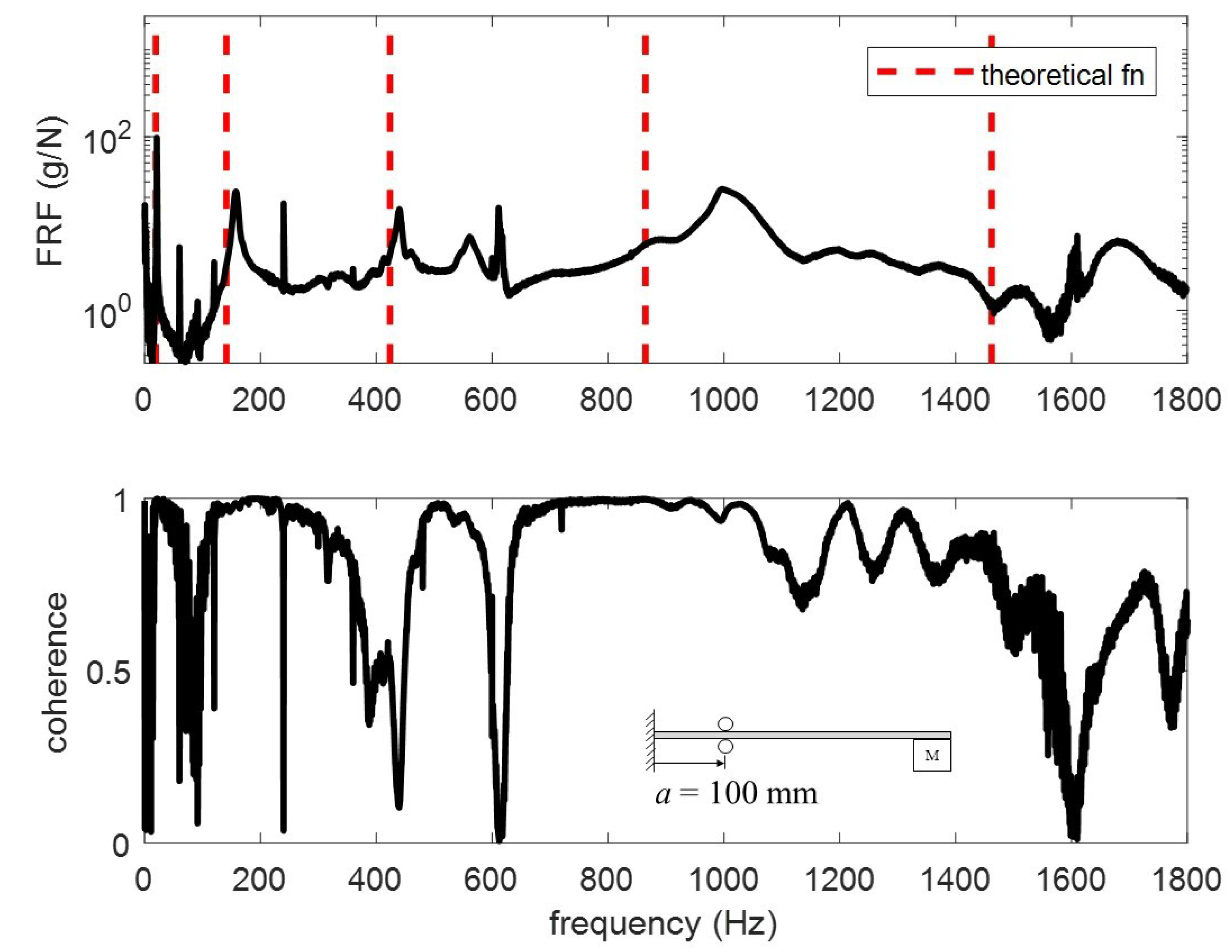
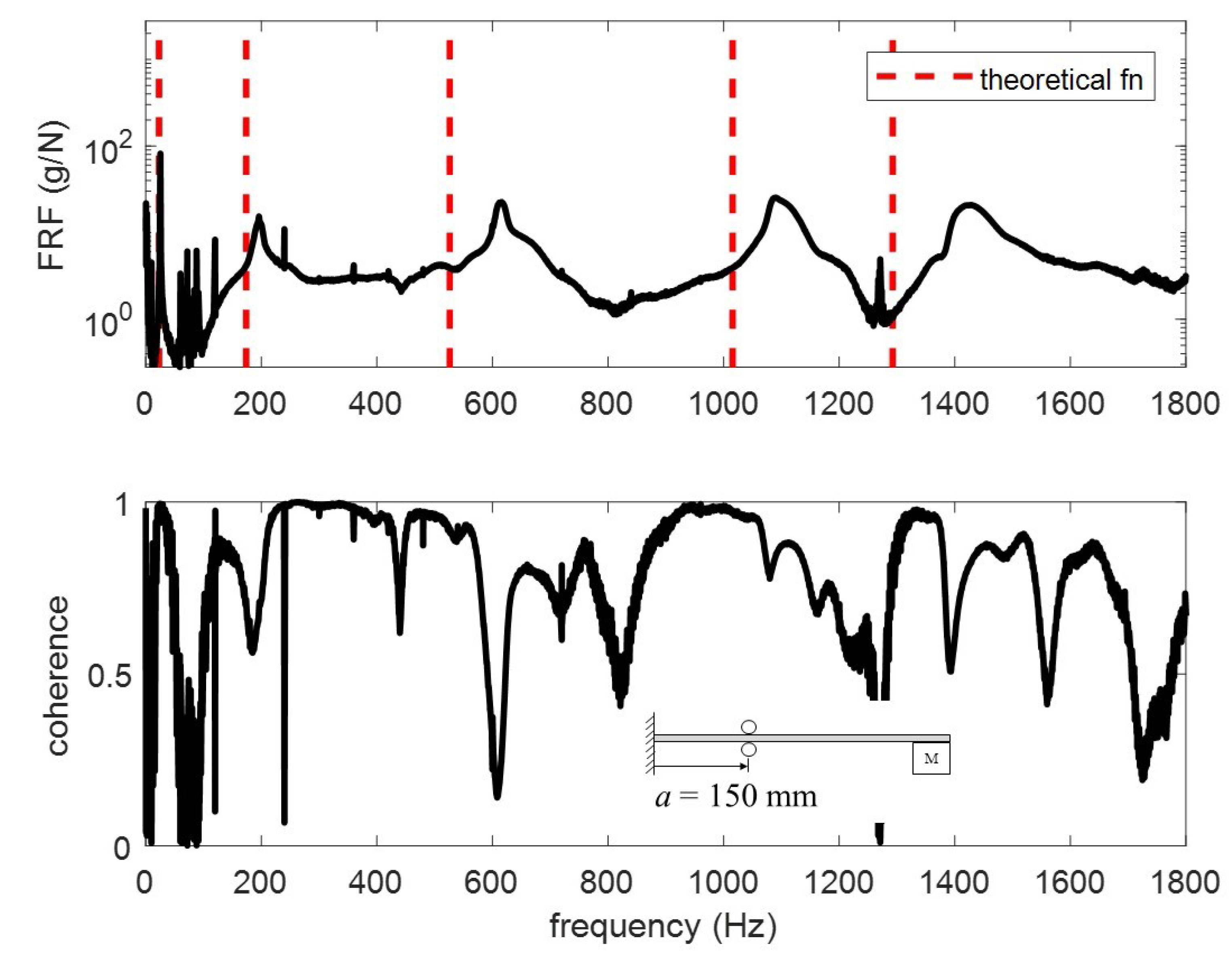
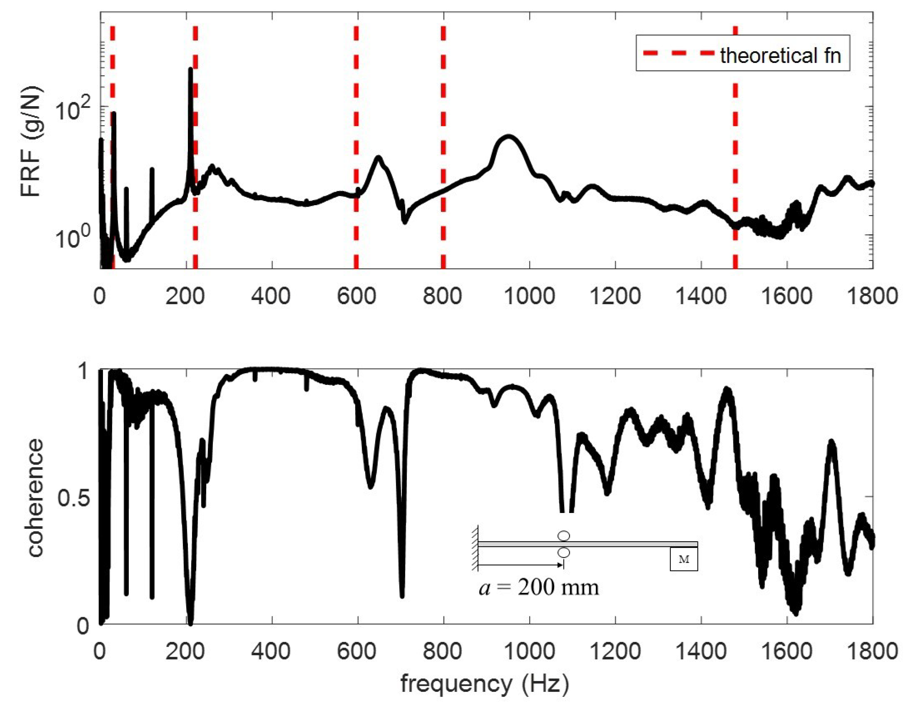
The accelerometers are single axis PCB 353B17. They are connected to a NI-9234 IEPE analog input module seated in an NI cDAQ-9172 chassis. A PCB 086C01 modal hammer with a white ABS plastic tip is used to excite the beam at 300 mm. Five tests under each condition are conducted and averaged in the frequency domain to generate frequency response functions (FRFs) using the $H_v$ algorithm [15]. The FRFs for the different tests are plotted in Figure 12, Figure 13, Figure 14 and Figure 15. The vertical red dashed lines represent the theoretical modes computed from the proposed model. To better understand the differences, the modes are extracted and tabulated in

Table 5. Pinned at $a=50$ mm and $\frac{m_{\mathrm{attached}}}{m_{\mathrm{beam}}}=0.2$.

	Proposed Model	Experiment	Difference
Mode	(Hz)	(Hz)	(%)
1	16.73	17.75	6.1
2	118.28	128.88	9.0
3	350.24	378.68	8.1
4	710.71	872.01	22.7
5	1202.46	1400.19	16.4

,

Table 6. Pinned at $a=100$ mm and $\frac{m_{\mathrm{attached}}}{m_{\mathrm{beam}}}=0.2$.

	Proposed Model	Experiment	Difference
Mode	(Hz)	(Hz)	(%)
1	19.48	21.37	9.7
2	141.29	157.37	11.4
3	423.53	440.11	3.9
4	864.86	996.16	15.2
5	1462.39	1680.39	14.9

,

Table 7. Pinned at $a=150$ mm and $\frac{m_{\mathrm{attached}}}{m_{\mathrm{beam}}}=0.2$.

	Proposed Model	Experiment	Difference
Mode	(Hz)	(Hz)	(%)
1	23.09	25.87	12.0
2	173.89	195.62	12.5
3	526.12	614.09	16.7
4	1015.61	1088.84	7.2
5	1292.51	1421.86	10.0

and

Table 8. Pinned at $a=200$ mm and $\frac{m_{\mathrm{attached}}}{m_{\mathrm{beam}}}=0.2$.

	Proposed Model	Experiment	Difference
Mode	(Hz)	(Hz)	(%)
1	28.02	31.39	12.0
2	221.20	259.65	17.4
3	595.97	646.99	8.6
4	798.79	950.15	18.9
5	1479.27	1741.16	17.7

.

For the four test conditions evaluated, the difference between the theoretical calculations and experimental results for modes 4 and 5 are non-trivial. Three possible explanations for these differences are (1) the electromagnet vibrates separate from the beam, (2) the beam vibrates within the rollers, and (3) the rotational inertia from a large mass at the end of a long beam impacts the higher frequencies. In Figure 13 and Figure 15, the coherence for mode 5 drops significantly such that it cannot be said with certainty that the frequencies are correct. Percent difference is used to quantify how different the theoretical frequencies are from the experimental. All frequencies fall below 20% difference with the exception of mode 4 in Table 5.

6. Conclusions

A high-rate experimental testbed is studied. The testbed is characterized as being a clamped-pinned-free beam with a mass at the free end. Euler-Bernoulli beam theory is applied to derive the transcendental equation for a general case applicable to the system pinned at an arbitrary location and with an arbitrary mass. The eigenvalues and mode shapes were presented under various test conditions. Experimental tests were conducted and results compared with the theoretical calculations of the first five natural frequencies. The comparison of results exhibited a good match in frequency values for the first three modes. The errors increase with the higher modes. The difference in higher modes can be attributed to the electromagnet vibrating separate to the beam, the beam vibrating within the rollers, and the rotational inertia of the mass not taken into consideration. Nevertheless, the percent difference of all modes between the theoretical and experimental values fell below 20% except for one case. These results confirm that within reason, the theory matches the experimental results.

The analytical model developed here can be useful in the design and numerical assessment of structural health monitoring solutions designed for systems operating in high-rate dynamic environments. Furthermore, the experimental quantification of the error in the higher modes validates and defines the bounds for which the high-rate experimental testbed is best utilized. Future work will include the evaluation of algorithms and methodologies for the SHM of structures experiences high-rate dynamic events.