Congestion-Free Ant Traffic: Jam Absorption Mechanism in Multiple Platoons


Abstract
1. Introduction
2. Model and Simulation Scenario
2.1. Model
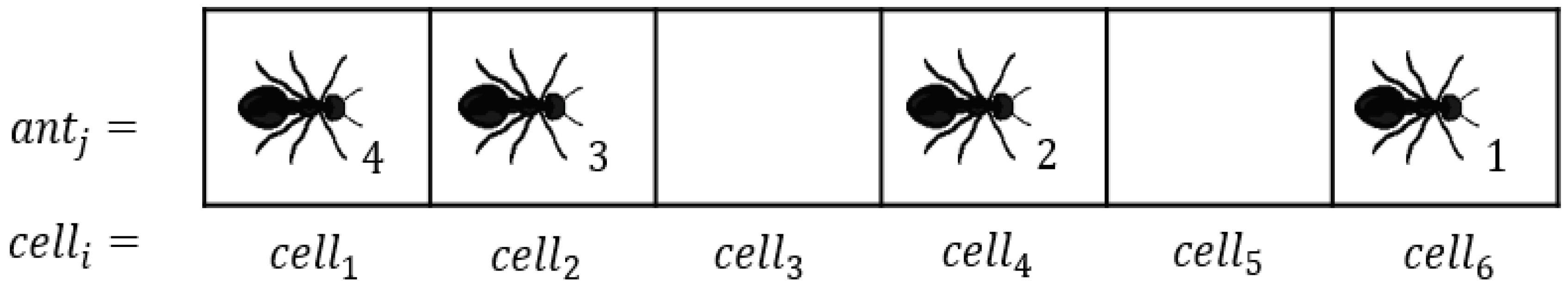
- The binary variable is either zero or one depending on whether the cell is empty (zero) or occupied (one) by an ant at time step t.
- The pheromone concentration is a numerical variable ranging from zero to . means that there is no pheromone in cell i at time step t, whereas means that the cell is saturated with pheromone at that time step.
- represents a resistance or drag that the cells present against the ant motion. represents factors related to trail conditions such as obstacle, rough trail, or uphill, which have a negative impact on the motion of ants. In short, provides opposition to the motion in the preferred direction, which is represented in ATM by a negative velocity (velocity in the opposite direction). In a given simulation, is constant for a given cell. To avoid ants moving backwards, is designed to always be positive, but less than the non-zero minimum ant velocity (as explained later, is used while defining the heterogeneous trail.).
- is the instantaneous velocity of ant j at time step t. is continuous and ranges from zero to one.
- is the position of ant j on the trail at time step t and ranges from zero to L. Similar to , is also continuous.
2.1.1. Stage I: Ant Motion
2.1.2. Stage II: Pheromone Updating
- Evaporation:
- Accumulation:
2.2. Simulation Scenarios
2.2.1. Periodic Boundary Conditions and Introduction of New Ants
2.2.2. Trail Scenarios
Homogeneous Trail
Heterogeneous Trail
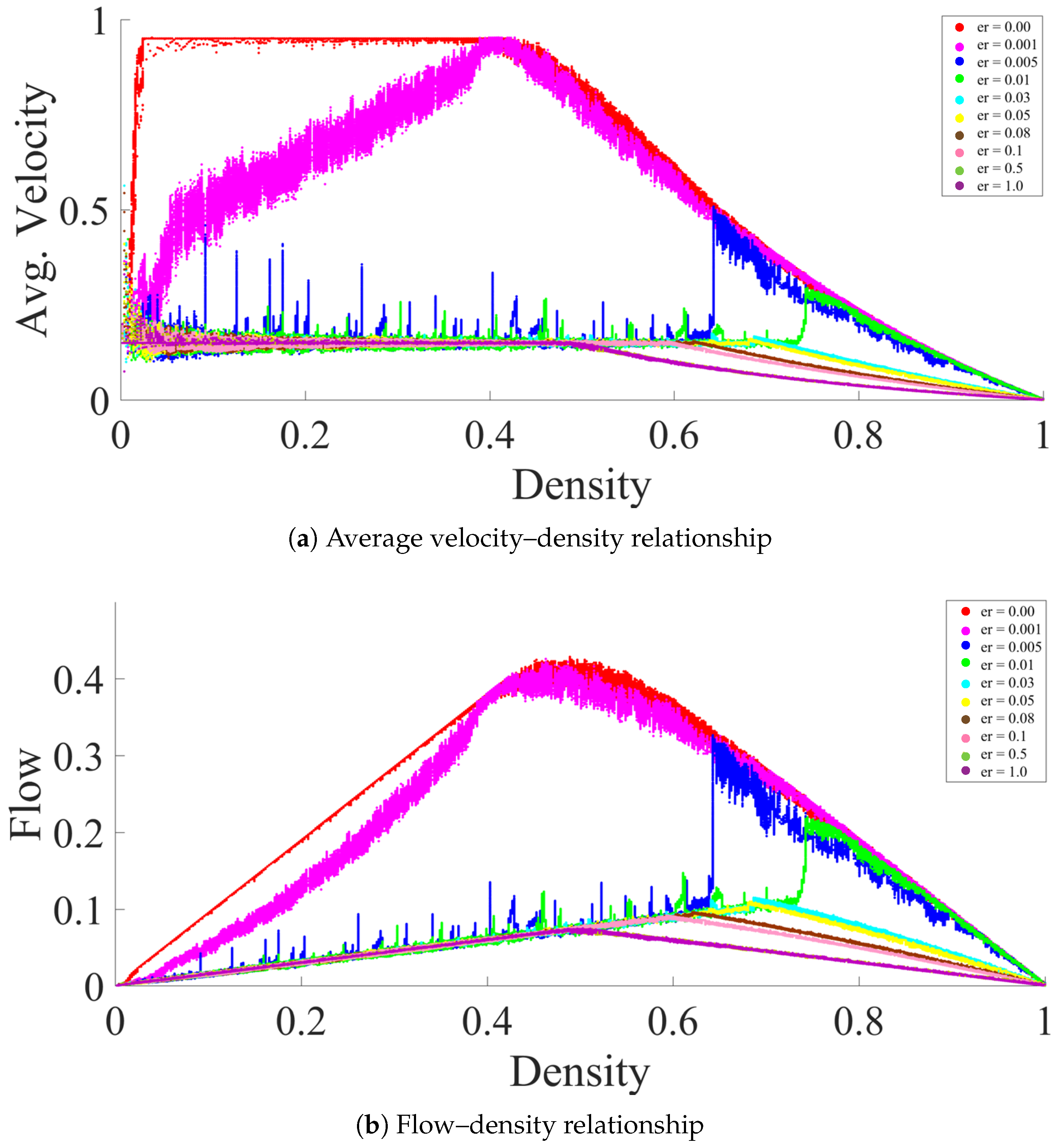
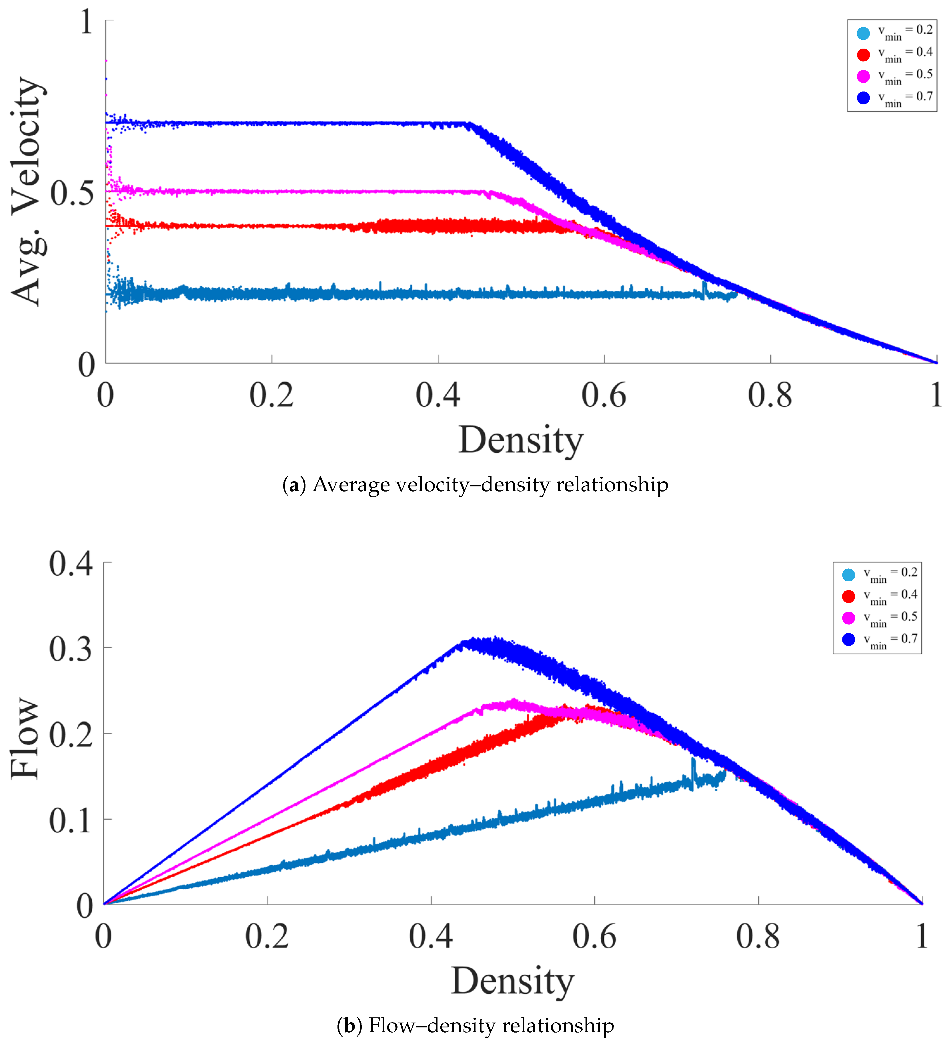
3. Fundamental Diagrams and Evaporation Rate
3.1. High to Medium Evaporation Rate ()
3.2. Meager Evaporation Rate ()
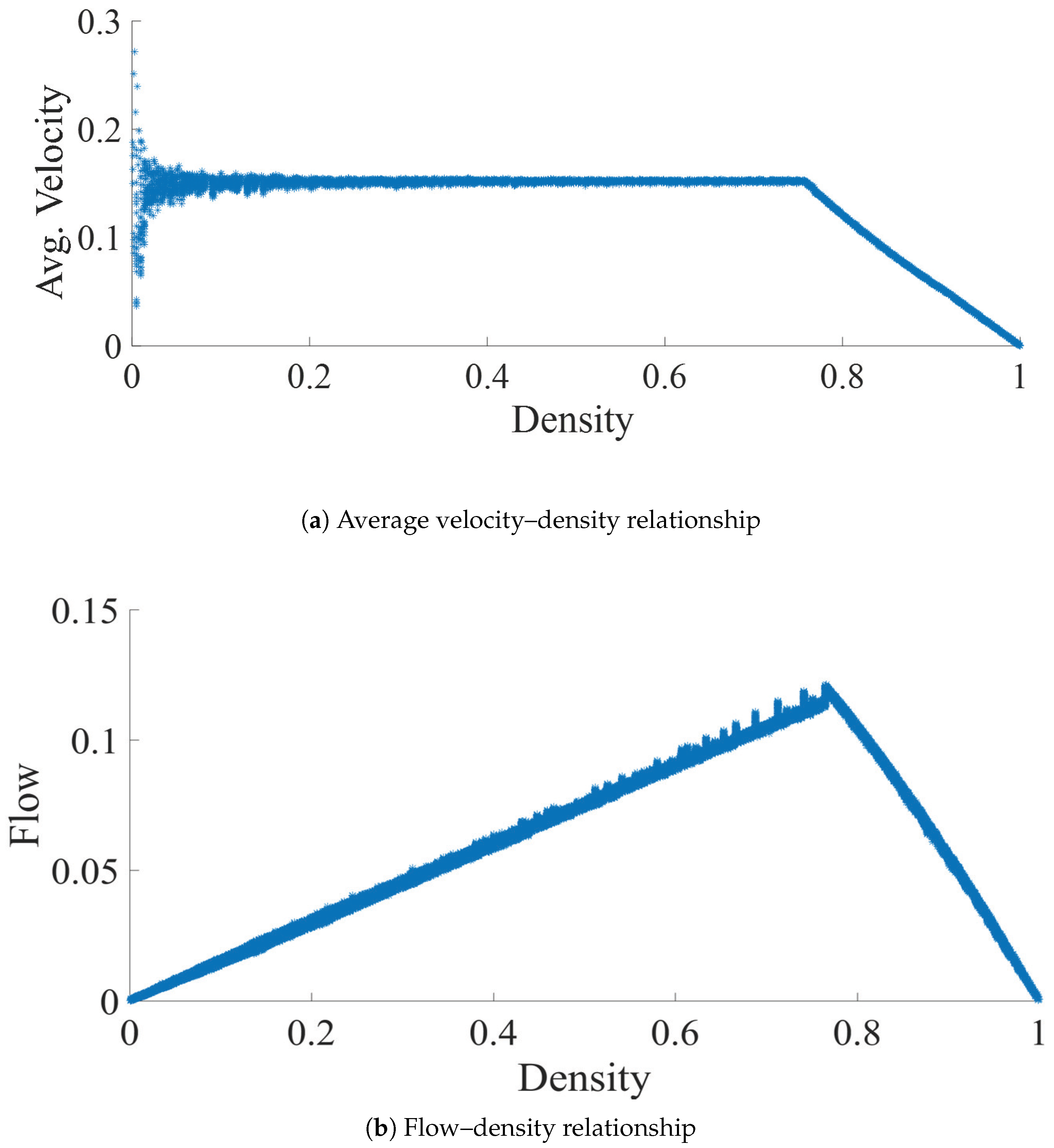
3.3. Low Evaporation Rate ()
4. Model Validation
5. Analysis of Jam-Free Ant Traffic
5.1. Intra-Platoon Analysis
5.2. Inter-Platoon Analysis
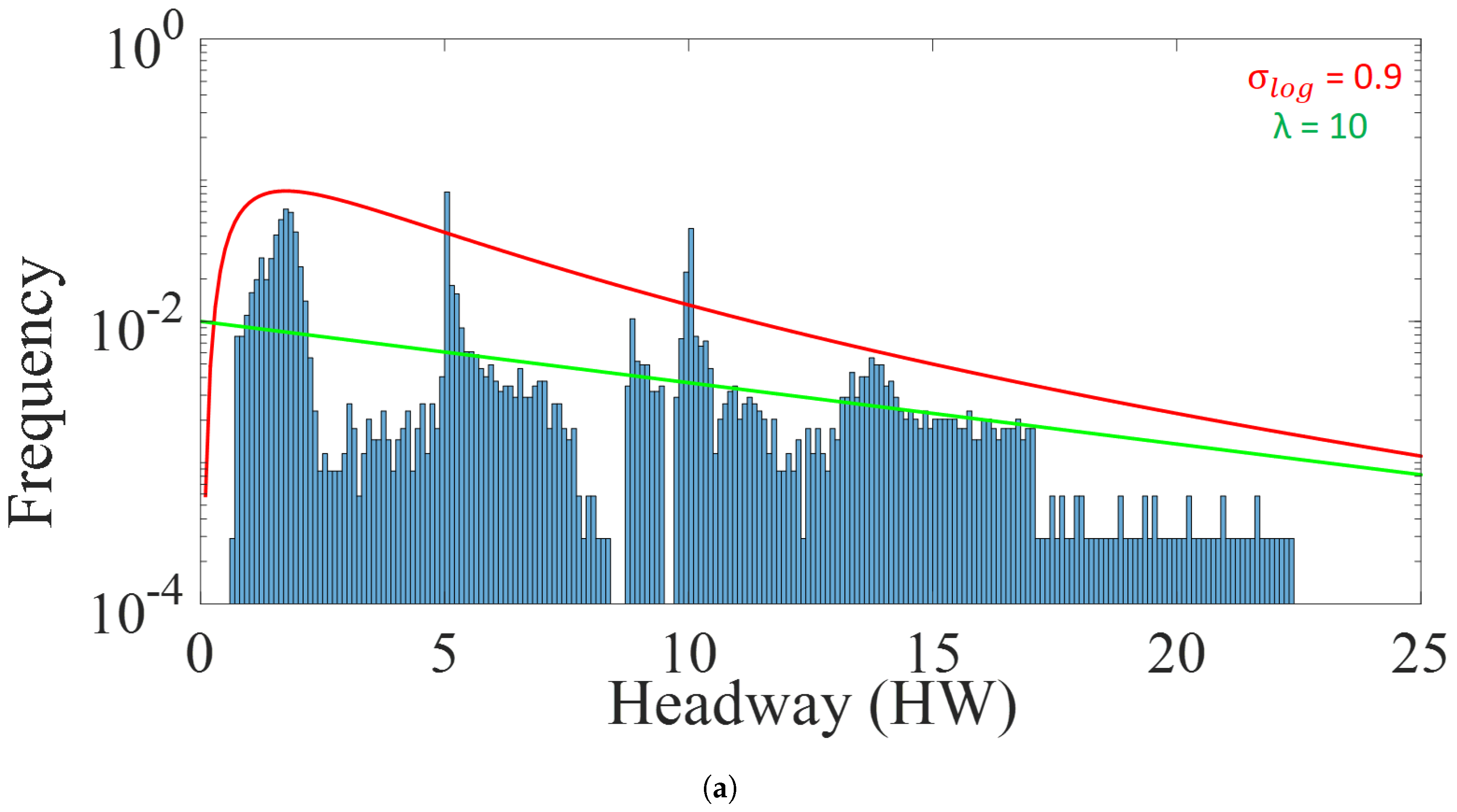
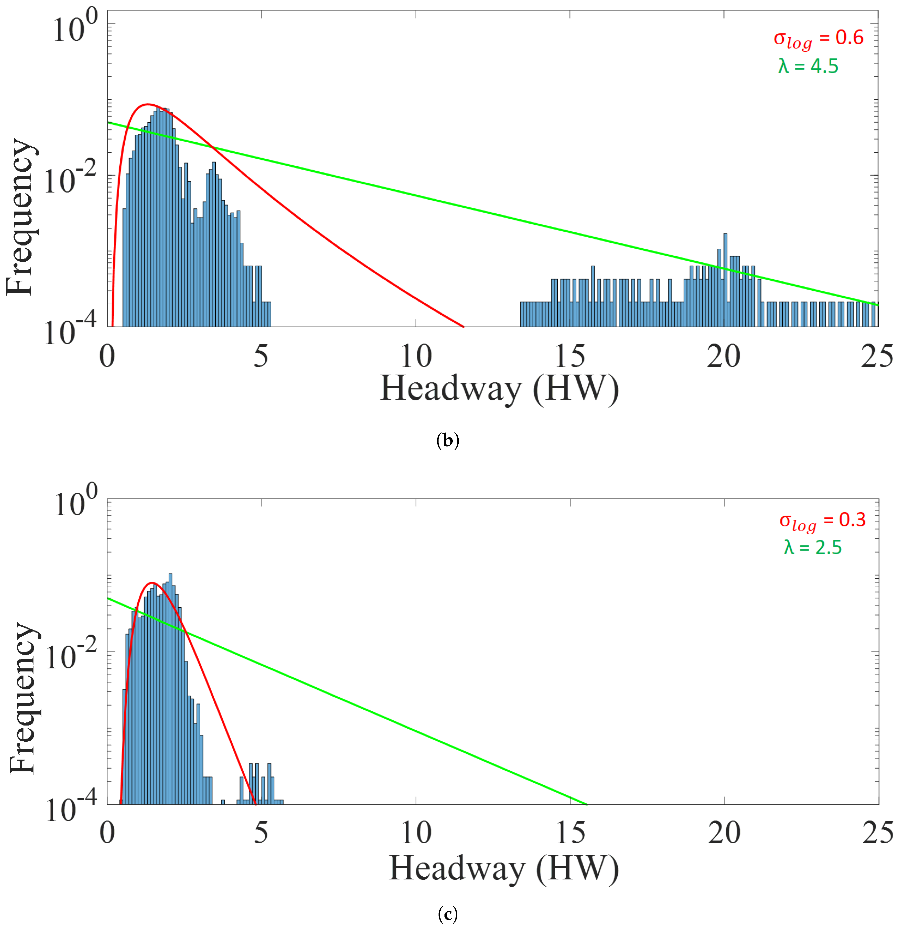
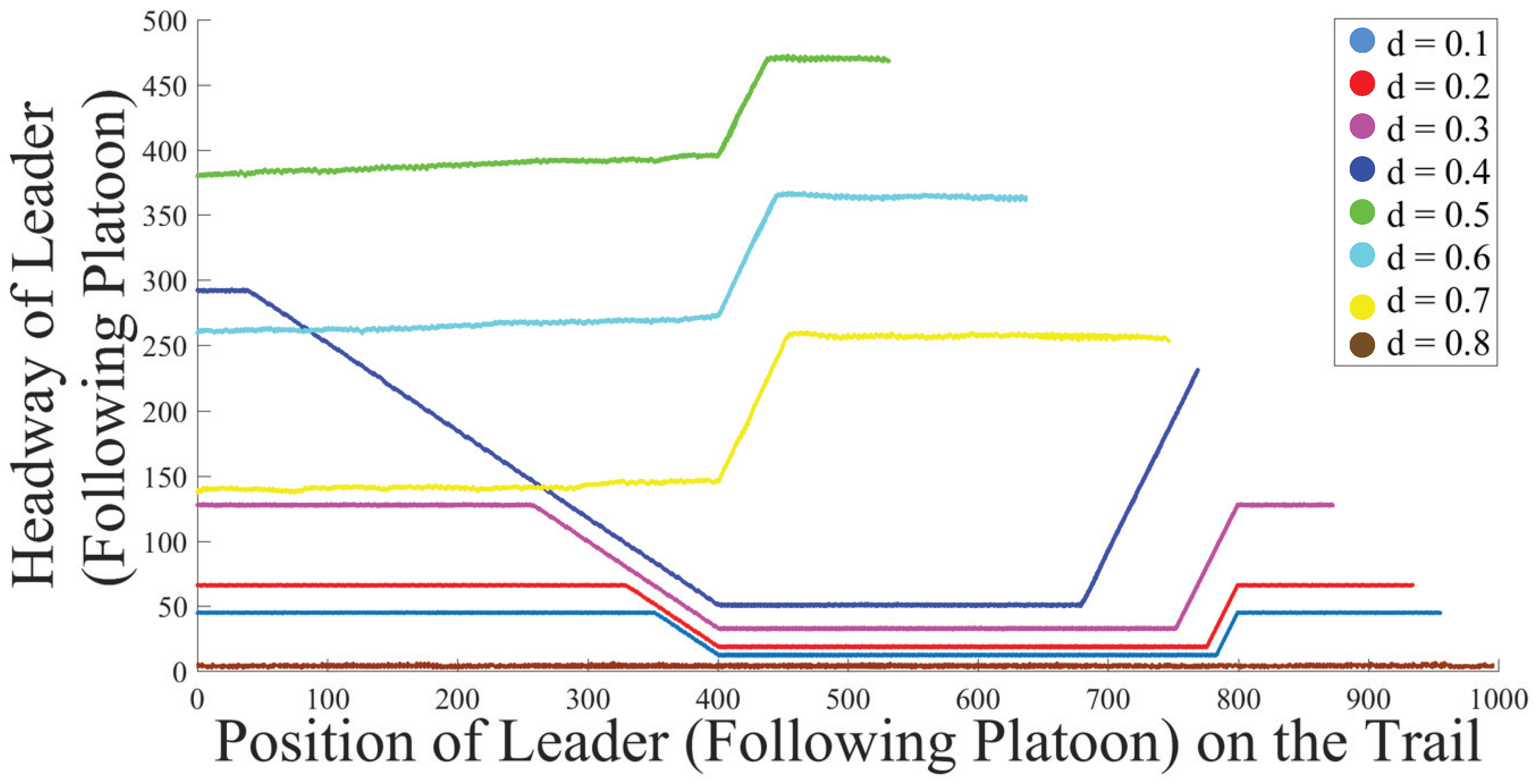
5.3. Analysis of Platoon Headway and Density
6. Concluding Discussion
Author Contributions
Funding
Conflicts of Interest
Appendix A. Variables in the Ant Trail Model
Appendix A.1. Minimum Velocity in ATM (vmin)

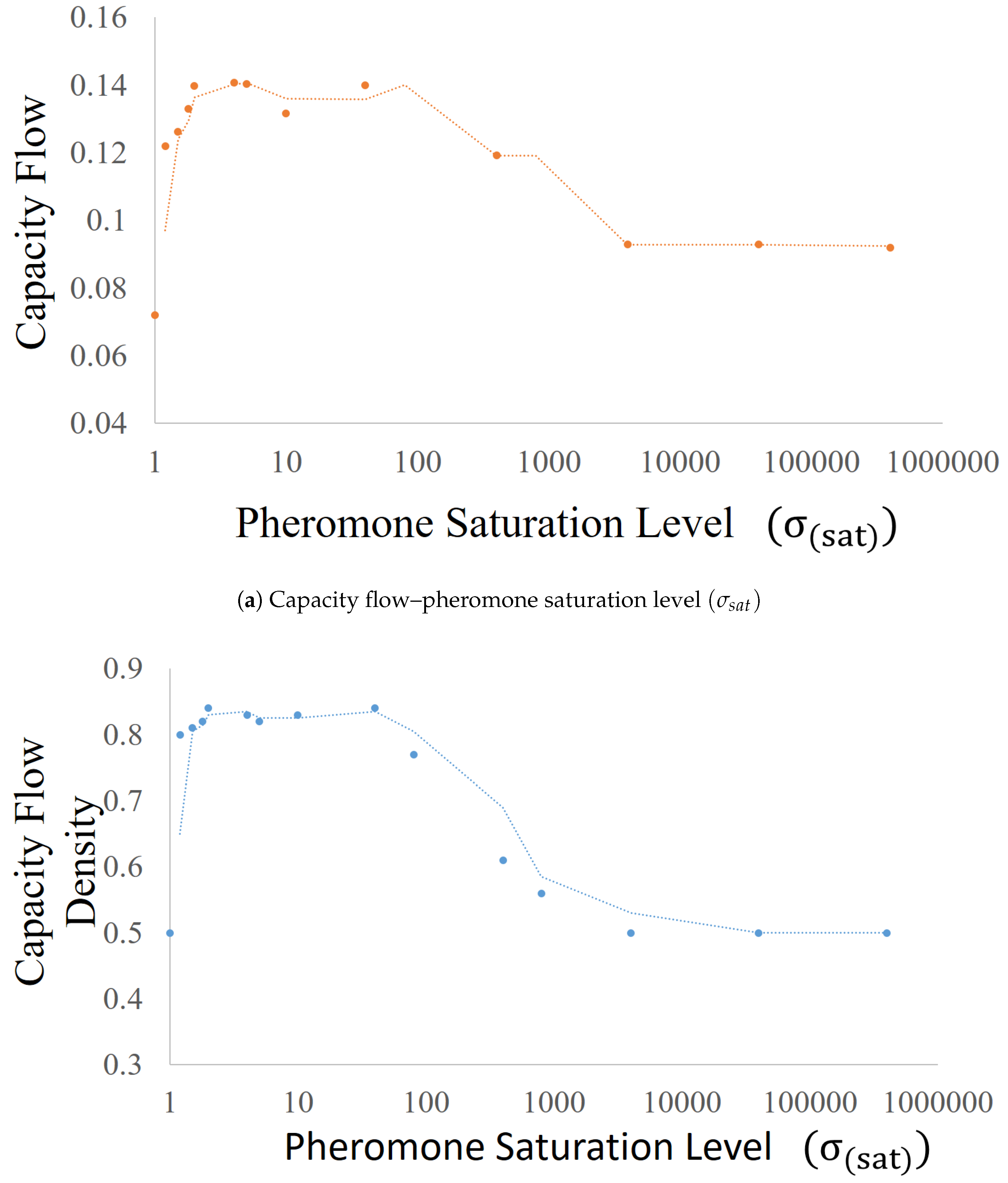
Appendix A.2. Pheromone Saturation Level (σsat)

References
- Khaluf, Y.; Ferrante, E.; Simoens, P.; Huepe, C. Scale invariance in natural and artificial collective systems: A review. J. R. Soc. Interface 2017, 14, 20170662. [Google Scholar] [CrossRef] [PubMed]
- Jennings, N.R. On agent-based software engineering. Artif. Intell. 2000, 117, 277–296. [Google Scholar] [CrossRef]
- Ponta, L.; Cincotti, S. Traders’ networks of interactions and structural properties of financial markets: An agent-based approach. Complexity 2018, 2018, 9072948. [Google Scholar] [CrossRef]
- Batty, M. Cities and Complexity: Understanding Cities with Cellular Automata, Agent-Based Models, and Fractals; The MIT Press: Cambridge, MA, USA, 2007. [Google Scholar]
- Chowdhury, D.; Schadschneider, A.; Nishinari, K. Physics of transport and traffic phenomena in biology: From molecular motors and cells to organisms. Phys. Life Rev. 2005, 2, 318–352. [Google Scholar] [CrossRef]
- Nishinari, K. Jamology: Physics of Self-Driven Particles and toward Solution of All Jams; Distributed Autonomous Robotic Systems 8; Springer: Berlin/Heidelberg, Germany, 2009; pp. 175–184. [Google Scholar]
- Chopard, B.; Droz, M. Cellular Automata Modeling of Physical Systems; Cambridge University Press: Cambridge, UK, 1998. [Google Scholar]
- Helbing, D. Traffic and related self-driven many-particle systems. Rev. Mod. Phys. 2001, 73, 1067. [Google Scholar] [CrossRef]
- Chowdhury, D.; Guttal, V.; Nishinari, K.; Schadschneider, A. A cellular-automata model of flow in ant trails: non-monotonic variation of speed with density. J. Phys. Math. Gen. 2002, 35, L573. [Google Scholar] [CrossRef]
- Couzin, I.D.; Franks, N.R. Self-organized lane formation and optimized traffic flow in army ants. Proc. R. Soc. Lond. Biol. Sci. 2003, 270, 139–146. [Google Scholar] [CrossRef] [PubMed]
- John, A.; Schadschneider, A.; Chowdhury, D.; Nishinari, K. Collective effects in traffic on bi-directional ant trails. J. Theor. Biol. 2004, 231, 279–285. [Google Scholar] [CrossRef]
- Nishinari, K.; Sugawara, K.; Kazama, T.; Schadschneider, A.; Chowdhury, D. Modelling of self-driven particles: Foraging ants and pedestrians. Phys. Stat. Mech. Its Appl. 2006, 372, 132–141. [Google Scholar] [CrossRef]
- Chaudhuri, D.; Nagar, A. Absence of jamming in ant trails: Feedback control of self-propulsion and noise. Phys. Rev. E 2015, 91, 012706. [Google Scholar] [CrossRef]
- John, A.; Schadschneider, A.; Chowdhury, D.; Nishinari, K. Trafficlike collective movement of ants on trails: Absence of a jammed phase. Phys. Rev. Lett. 2009, 102, 108001. [Google Scholar] [CrossRef] [PubMed]
- Guo, N.; Hu, M.B.; Jiang, R.; Ding, J.; Ling, X. Modeling no-jam traffic in ant trails: A pheromone-controlled approach. J. Stat. Mech. Theory Exp. 2018, 2018, 053405. [Google Scholar] [CrossRef]
- Garnier, S.; Guérécheau, A.; Combe, M.; Fourcassié, V.; Theraulaz, G. Path selection and foraging efficiency in Argentine ant transport networks. Behav. Ecol. Sociobiol. 2009, 63, 1167–1179. [Google Scholar] [CrossRef]
- Vittori, K.; Talbot, G.; Gautrais, J.; Fourcassié, V.; Araújo, A.F.; Theraulaz, G. Path efficiency of ant foraging trails in an artificial network. J. Theor. Biol. 2006, 239, 507–515. [Google Scholar] [CrossRef] [PubMed]
- Chowdhury, D.; Santen, L.; Schadschneider, A. Statistical physics of vehicular traffic and some related systems. Phys. Rep. 2000, 329, 199–329. [Google Scholar] [CrossRef]
- Goss, S.; Aron, S.; Deneubourg, J.L.; Pasteels, J.M. Self-organized shortcuts in the Argentine ant. Naturwissenschaften 1989, 76, 579–581. [Google Scholar] [CrossRef]
- Beckers, R.; Deneubourg, J.L.; Goss, S. Trails and U-turns in the selection of a path by the ant Lasius niger. J. Theor. Biol. 1992, 159, 397–415. [Google Scholar] [CrossRef]
- Hölldobler, B.; Wilson, E.O. The Ants; Harvard University Press: Cambridge, MA, USA, 1990. [Google Scholar]
- Wilson, E.O. The Insect Societies; [Distributed by Oxford University Press]; Harvard University Press: Cambridge, MA, USA, 1971. [Google Scholar]
- Camazine, S.; Deneubourg, J.L.; Franks, N.R.; Sneyd, J.; Bonabeau, E.; Theraula, G. Self-Organization in Biological Systems; Princeton University Press: Princeton, NJ, USA, 2003; Volume 7. [Google Scholar]
- Andryszak, N.; Payne, T.L.; Dickens, J.; Moser, J.C.; Fisher, R. Antennal olfactory responsiveness of the Texas leaf cutting ant (Hymenoptera: Formicidae) to trail pheromone and its two alarm substances. J. Entomol. Sci. 1990, 25, 593–600. [Google Scholar] [CrossRef]
- Czaczkes, T.J.; Grüter, C.; Ellis, L.; Wood, E.; Ratnieks, F.L. Ant foraging on complex trails: Route learning and the role of trail pheromones in Lasius niger. J. Exp. Biol. 2013, 216, 188–197. [Google Scholar] [CrossRef]
- Nishinari, K.; Chowdhury, D.; Schadschneider, A. Cluster formation and anomalous fundamental diagram in an ant-trail model. Phys. Rev. E 2003, 67, 036120. [Google Scholar] [CrossRef]
- Kunwar, A.; John, A.; Nishinari, K.; Schadschneider, A.; Chowdhury, D. Collective traffic-like movement of ants on a trail: dynamical phases and phase transitions. J. Phys. Soc. Jpn. 2004, 73, 2979–2985. [Google Scholar] [CrossRef]
- Tisue, S.; Wilensky, U. Netlogo: A simple environment for modeling complexity. In Proceedings of the International Conference on Complex Systems, Boston, MA, USA, 16–21 May 2004; Volume 21, pp. 16–21. [Google Scholar]
- Schadschneider, A. The nagel-schreckenberg model revisited. Eur. Phys. J. B-Condens. Matter Complex Syst. 1999, 10, 573–582. [Google Scholar] [CrossRef]
- Nishi, R.; Tomoeda, A.; Shimura, K.; Nishinari, K. Theory of jam-absorption driving. Transp. Res. Part B Methodol. 2013, 50, 116–129. [Google Scholar] [CrossRef]
- Taniguchi, Y.; Nishi, R.; Ezaki, T.; Nishinari, K. Jam-absorption driving with a car-following model. Phys. A Stat. Mech. Its Appl. 2015, 433, 304–315. [Google Scholar] [CrossRef]


| Description | Symbol |
|---|---|
| Unique identity of a cell in the trail | i |
| Presence or absence of an ant in the trail at time t | |
| Pheromone concentration in the trail at time t | |
| Resistance by the trail to the motion of an ant | |
| Pheromone concentration saturation level | |
| Unique identity of an ant in the simulation | j |
| Velocity of the at time t | |
| Position of the at time t | |
| Minimum velocity of an ant towards the cell with no pheromone and no other ant | |
| Trail length | L |
| Evaporation rate |
| Description | Simulation Values |
|---|---|
| Pheromone concentration saturation level | |
| Resistance from the trail to the motion of an agent in the homogeneous trail scenario | |
| Resistance from the trail in the high resistance section to the motion of an ant in the heterogeneous trail scenario | |
| Minimum velocity of an ant towards the cell with no pheromone and no other ant | |
| Trail length | |
| Inflow rate | = 0.001 |
| Evaporation rate | |
| High resistance trail section in the heterogeneous trail scenario | – |
| Density | Number of Platoons |
|---|---|
| 0.1 | 28 |
| 0.2 | 21 |
| 0.3 | 14 |
| 0.4 | 8 |
| 0.5 | 3 |
| 0.6 | 3 |
| 0.7 | 2 |
| 0.8 | 1 |
© 2019 by the authors. Licensee MDPI, Basel, Switzerland. This article is an open access article distributed under the terms and conditions of the Creative Commons Attribution (CC BY) license (http://creativecommons.org/licenses/by/4.0/).
Share and Cite
Kasture, P.; Nishimura, H. Congestion-Free Ant Traffic: Jam Absorption Mechanism in Multiple Platoons. Appl. Sci. 2019, 9, 2918. https://doi.org/10.3390/app9142918
Kasture P, Nishimura H. Congestion-Free Ant Traffic: Jam Absorption Mechanism in Multiple Platoons. Applied Sciences. 2019; 9(14):2918. https://doi.org/10.3390/app9142918
Chicago/Turabian StyleKasture, Prafull, and Hidekazu Nishimura. 2019. "Congestion-Free Ant Traffic: Jam Absorption Mechanism in Multiple Platoons" Applied Sciences 9, no. 14: 2918. https://doi.org/10.3390/app9142918
APA StyleKasture, P., & Nishimura, H. (2019). Congestion-Free Ant Traffic: Jam Absorption Mechanism in Multiple Platoons. Applied Sciences, 9(14), 2918. https://doi.org/10.3390/app9142918