Deep Homography Estimation and Its Application to Wall Maps of Wall-Climbing Robots

Featured Application

This study focused on the homography estimation between the camera image and the wall map and presented a novel method (HomographyFpnNet). The high precision and low time consumption of this method will benefit many homography-related applications in robotics and computer vision, such as image stitching, simultaneous localization and mapping (SLAM), 3D reconstruction and optical flow.

Abstract

When locating wall-climbing robots with vision-based methods, locating and controlling the wall-climbing robot in the pixel coordinate of the wall map is an effective alternative that eliminates the need to calibrate the internal and external parameters of the camera. The estimation accuracy of the homography matrix between the camera image and the wall map directly impacts the pixel positioning accuracy of the wall-climbing robot in the wall map. In this study, we focused on the homography estimation between the camera image and wall map. We proposed HomographyFpnNet and obtained a smaller homography estimation error for a center-aligned image pair compared with the state of the art. The proposed hierarchical HomographyFpnNet for a non-center-aligned image pair significantly outperforms the method based on artificially designed features + Random Sample Consensus. The experiments conducted with a trained three-stage hierarchical HomographyFpnNet model on wall images of climbing robots also achieved small mean corner pixel error and proved its potential for estimating the homography between the wall map and camera images. The three-stage hierarchical HomographyFpnNet model has an average processing time of 10.8 ms on a GPU. The real-time processing speed satisfies the requirements of wall-climbing robots.

1. Introduction

In the past several decades, considerable research has been dedicated to the development of mobile systems that can traverse vertical surfaces. This research on wall-climbing robots has predominantly been motivated by increases in safety legislation and economic efficiency improvements over existing solutions. Wall-climbing robots can replace humans in the execution of highly dangerous tasks [1,2,3,4,5,6,7], such as evaluating and diagnosing storage tanks in petrochemical facilities and nuclear power plants, inspecting and cleaning high-rise buildings, performing the maintenance and welding of ship hulls and application in open-pit mine walls. It can be seen that wall-climbing robots are widely used in a variety of engineering applications.

Accurate location detection is important in the controlling of wall-climbing robots, and visual methods are commonly used in the positioning of wall-climbing robots [8,9,10]. In these methods, the wall-climbing robot is first detected visually, and the pixel position of the robot must then be converted for use in a spatial coordinate system of the wall according to the calibrated external parameters of the camera. To convert the pixel position to a spatial coordinate, the rotation matrix $\mathbf{R}$ and translation matrix $\mathbf{t}$ of the coordinate system of the camera are calibrated against a coordinate system of the wall. However, when the camera is far away from the wall (e.g., 20 m), it is difficult to calibrate the external parameters of the camera. A simple and effective alternative is to prepare a wall map (using the front view of the wall), and to then locate and control the climbing robot using the pixel coordinate of the wall map, as shown in Figure 1. To locate and control wall-climbing robots using a wall map, the pixel coordinate of the wall-climbing robot, as detected in image_a (Figure 1, left), can be translated as a pixel coordinate in wall_map (Figure 1, right) using a homography matrix (or projective transformation matrix) H, which eliminates the need to calibrate the internal and external parameters of the camera. Obstacles can also be labeled on the wall to assist in the design of a safe walking route for the wall-climbing robot.

The estimation accuracy of H between the camera image and the wall map directly impacts the pixel positioning accuracy of the wall-climbing robot in the wall map. This paper focuses on the homography estimation between the camera image and the wall map. Direct Linear Transformation (DLT) based on two sets of corresponding points including at least four pairs of corresponding points is the basic method of homography estimation, but finding corresponding points from a given pair of images is difficult. The usual practice is to use artificially designed features (e.g., Scale-Invariant Feature Transform (SIFT) [11] and Oriented FAST and Rotated BRIEF (ORB) [12]) to look for points of interest in the image first, and then to match the points of interest of the image pairs using a matching method to get two sets of corresponding points. Finally, Random Sample Consensus (RANSAC) [13] is used to process any incorrect matching point pairs that may exist in the point set. The best homography estimation is then selected after iterative optimization.

The requirement of artificially designed features and an exhaustive matching step are major issues with methods such as ORB+RANSAC. The deep learning model automatically extracts features and provides more powerful features than traditional methods. The superiority of feature extraction using deep learning models has been validated in a variety of tasks [14,15,16,17]. Recently, attempts have been made to solve the problem of matching using a Convolutional Neural Network (CNN). As an example, Flownet [18] solves the optical flow estimation task by using a parallel convolutional network model and a correlation layer. Flownet 2.0 [19] proposes a hierarchical model that is stacked by Flownet and achieves higher precision than Flownet.

Our contributions in this work are as follows: (1) we proposed HomographyFpnNet to improve the homography estimation accuracy of a center-aligned image pair; (2) based on the proposed HomographyFpnNet, we used a hierarchical method composed of one HomographyFpnNet_A model and two HomographyFpnNet_B models to estimate the homography of a non-center-aligned image pair, and the mean corner error was significantly smaller than that of the classical ORB/SIFT+RANSAC methods; and (3) we conducted experiments with our trained three-stage hierarchical HomographyFpnNet model on climbing robot wall images and achieved promising results.

The code is available at: https://github.com/ZJUZQ/HomographyFpnNet.

2. Related Work

Some attempts have been made to use CNN to solve the homography estimation; these attempts obtained higher estimation precision than the ORB+RANSAC method. DeTone et al. [20] proposed four-point homography, which is defined by four pairs of corresponding points between two images. The model proposed in [20] is similar to the VGG (Visual Geometry Group) architecture [21] with eight convolutional layers, one max pooling layer after every two convolutional layers, two fully connected layers and an L2 loss function that is calculated from the square of the difference between the predicted and the ground truth four-point coordinate values. Nowruzi et al. [22] proposed a hierarchical model that is stacked by the twin convolutional regression networks to estimate the homography between a pair of images, and improved the prediction accuracy of four-point homography compared with that of the work by DeTone et al. [20].

DeTone et al. and Nowruzi et al. [20,22] focused on estimating the homography between pairs of image_patch_a and image_patch_b with centers being roughly aligned, which we call center-aligned image pairs. However, in our task, we need to estimate the homography between image_a and image_patch_b when their centers are not necessarily aligned, as shown in Figure 2. We call these non-center-aligned image pairs, and they are more difficult, as we do not know which region of image_a should be matched with image_patch_b. The homography estimation of a center-aligned image pair is a special case of the homography estimation of a non-center-aligned image pair.

Because deep networks require many data to train from scratch, we took a similar approach as that used by DeTone et al. and Nowruzi et al. [20,22] to generate a seemingly infinite dataset for the homography estimation of center-aligned and non-center-aligned image pairs from the Microsoft Common Objects in Context (MS-COCO) [23] dataset. The trained models were then directly used for the homography estimation of climbing robot wall maps.

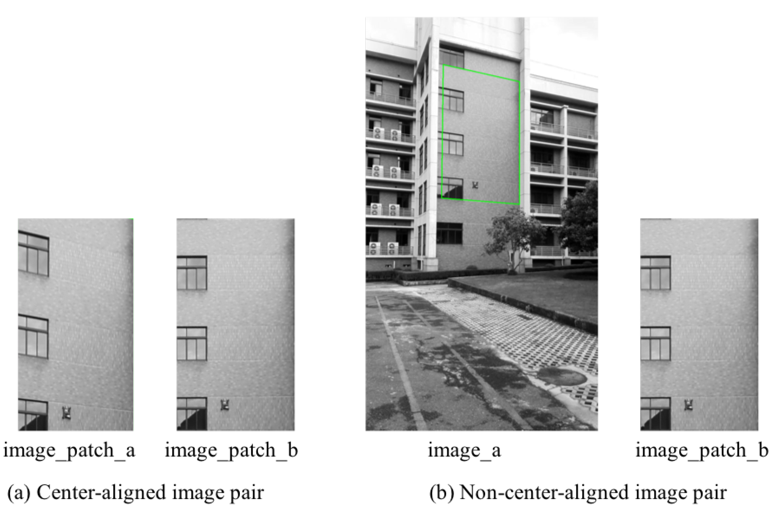
3. Homography Estimation for a Center-Aligned Image Pair

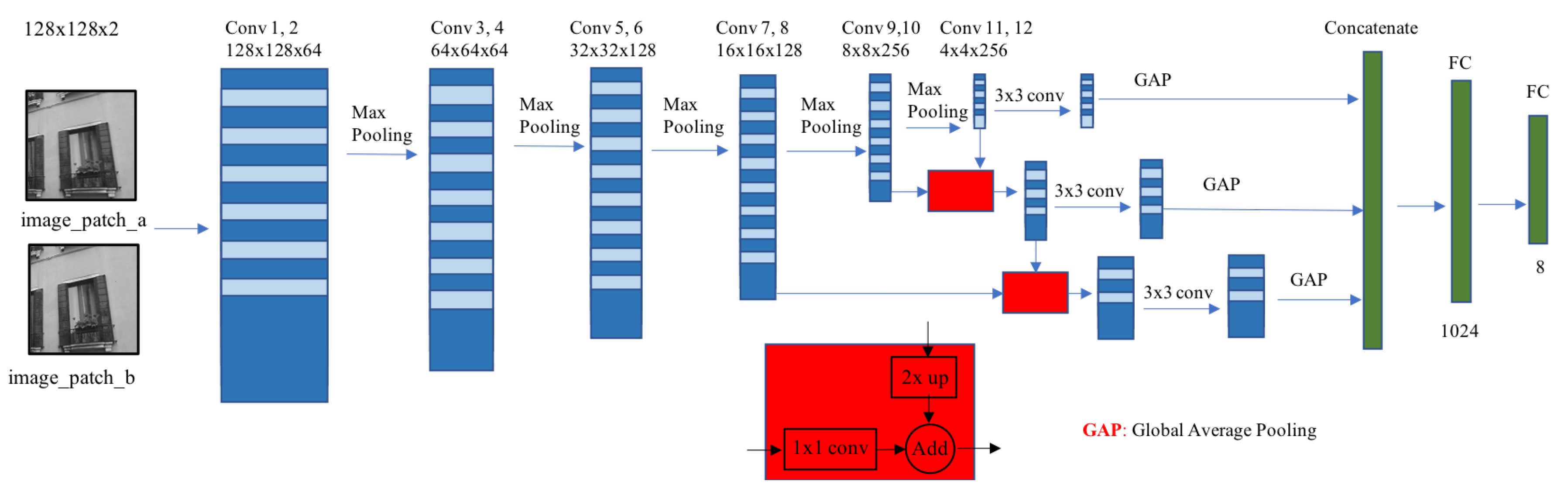
3.1. HomographyFpnNet Structure

Figure 3 shows the structure diagram of our regression-based HomographyFpnNet model for predicting the pixel offsets of the four corners of image_patch_b relative to those of image_patch_a when image_patch_b is warped to image_patch_a. HomographyFpnNet uses the VGG architecture (the deep convolutional network developed by Oxford’s Visual Geometry Group (VGG) for object recognition, which is characterized by its simplicity, using only $3\times 3$ convolutional layers stacked on top of each other to increase the depth of the network and using max pooling layers to reduce the dimensionality of the feature maps) [21], which was also used by HomographyNet [20]. The model input is a two-channel image of size $128\times 128\times 2$ pixels. In other words, the two grayscale input images associated by the homography transformation are stacked in a channel manner and fed into the model network. After extracting features through stacked convolutional layers, HomographyNet [20] uses the features of the last convolutional layer to predict the four-point homography values through two fully connected layers, meaning that HomographyNet only uses single-scale convolutional features. In contrast, the ORB+RANSAC method commonly uses multi-scale ORB features to improve the accuracy of its homography estimation. Inspired by this, we propose the use of multi-scale deep convolution features for the homography estimation. Specifically, as shown in Figure 3, we used Feature Pyramid Network (FPN) [24] to fuse the convolution features of three different scales, and then globally averaged and concatenated these three scale convolution features ($4\times 4$, $8\times 8$, and $16\times 16$) to obtain the final one-dimensional features. That is, the $4\times 4$ feature map of conv12’s output is upsampled to $8\times 8$ and then merged with the $8\times 8$ feature map of conv10’s output (which undergoes a $1\times 1$ convolutional layer to adjust channel number to 256) by element-wise addition to generate new $8\times 8$ feature map. Similarly, the new $8\times 8$ feature map is upsampled and then merged with the $16\times 16$ feature map of conv8’s output to generate new $16\times 16$ feature map. To reduce the aliasing effect of upsampling, each merged map undergoes a $3\times 3$ convolutional layer to generate the final feature map. Finally, as in HomographyNet, two fully connected layers are used for the regression of the four-point homography values.

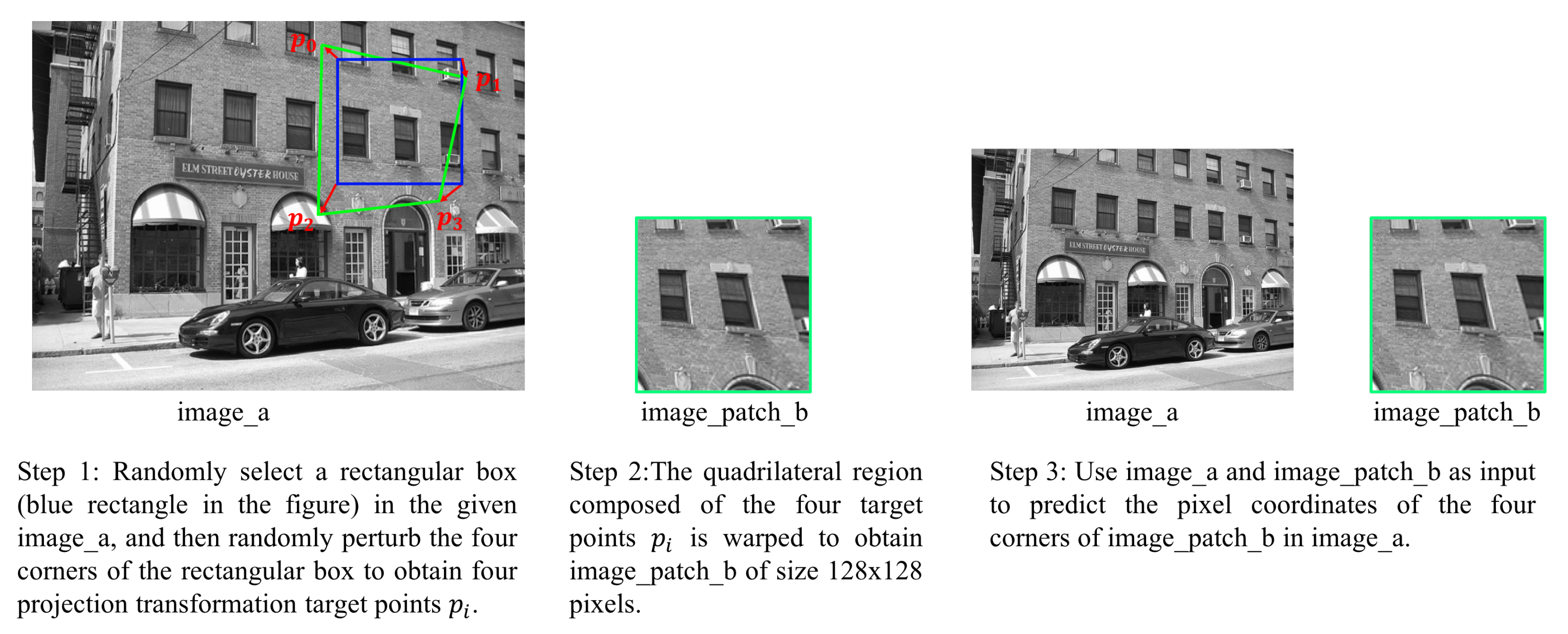
3.2. Dataset of the Center-Aligned Image Pair

Following other researchers [20,22], we also used the MS-COCO 2014 dataset. We selected 118,000 images from the trainval set of the MS-COCO 2014 dataset to prepare training samples and 10,000 images from the test set of the MS-COCO 2014 dataset to prepare test samples. First, we converted all the images selected from the MS-COCO 2014 dataset into single-channel gray-scale images and down-sampled the converted images to a resolution of $320\times 240$ pixels. Then, to increase the capacity of the resulting training set and test set, we generated three samples from each selected image. To achieve this, three rectangles of size $128\times 128$ pixels were randomly selected from the central area of each image (excluding the boundary area of 32 pixels). A random perturbation with a maximum absolute value of 32 pixels was added to the pixel coordinates of each corner of the rectangle, and the perturbation values of the four corners were the target four-point homography values. Then, we used the OpenCV library and the target homography values to warp the original image. Finally, we extracted the patches from the original image and the warped image using the pixel coordinates of the original four corners. The pair of extracted patches together with the target four-point homography values were fed as inputs to the network.

3.3. Training and Results

When training the HomographyFpnNet model, we used a momentum optimizer with a momentum value of 0.9, a batch size of 64, and an initial learning rate of 0.05. During the first 1000 training iteration steps, we linearly increased the learning rate from 0.0 to the initial learning rate of 0.05. We then continued training the model for an additional 90,000 iteration steps and simultaneously updated the learning rate from 0.05 to 0.0 using a cosine decay method [25].

We tested the mean corner error of the trained model on the 30,000 test samples generated from the COCO 2014 test dataset. The mean corner error was obtained based on the calculation of the L2 distance between the estimated and the ground truth corner locations, for the average of the four corners and all test samples. As shown in Figure 4, our HomographyFpnNet model had a mean corner error of 3.22 pixels on the 30,000 test samples generated from the MS-COCO 2014 test set. Compared with HomographyNet, the mean corner error decreased from 9.42 pixels (our own implementation, 9.2 pixels in the published report [20]) to 3.22 pixels, that is, the mean corner error decreased by 65%. Compared with the hierarchical method [22], our HomographyFpnNet model with an error of 3.22 pixels performed better than their four-stage model with an error of 3.91.

Figure 5 shows some of the prediction results of HomographyFpnNet on some MS-COCO 2014 dataset images and the associated wall images of our wall-climbing robots.

4. Homography Estimation for a Non-Center-Aligned Image Pair

We extended our study to estimate the homography for a non-center-aligned image pair and used the MS-COCO 2014 dataset to generate enough training and test samples for network model training and testing. The trained models were used to directly estimate the four-point homography between the camera images and the wall maps of wall-climbing robots in the next section.

4.1. Dataset of Non-Center-Aligned Image Pair

We chose 118,000 images from the trainval set of the MS-COCO 2014 dataset to generate training samples for the homography estimation, and 10,000 images from the test set of the MS-COCO 2014 dataset to generate test samples. As shown in Step 1 in Figure 6, all images selected from the MS-COCO 2014 dataset were converted to single-channel gray-scale images and three samples were generated from each selected image to increase the capacity of the resulting dataset. To do this, three rectangles (blue rectangle in Figure 6) of size $w\times h$ ($w\ge 128,h\ge 128$), excluding a boundary region of $\frac{w}{4}$ pixels in the x-direction and $\frac{h}{4}$ pixels in the y-direction, were randomly selected from each image. A random perturbation in the range of $\frac{w}{4}$ pixels for the x-coordinate and $\frac{h}{4}$ for the y-coordinate was added to the pixel coordinates of each corner of the rectangle, and the perturbation values of the four corners were the target four-point homography values (green quadrilaterals in Figure 6). In Step 2, the target four-point homography was warped to generate image_patch_b of size $128\times 128$ pixels. In Step 3, the image_a (resized to $128\times 128$ pixels) and image_patch_b pair, along with the target four-point homography values, were fed as inputs to the network.

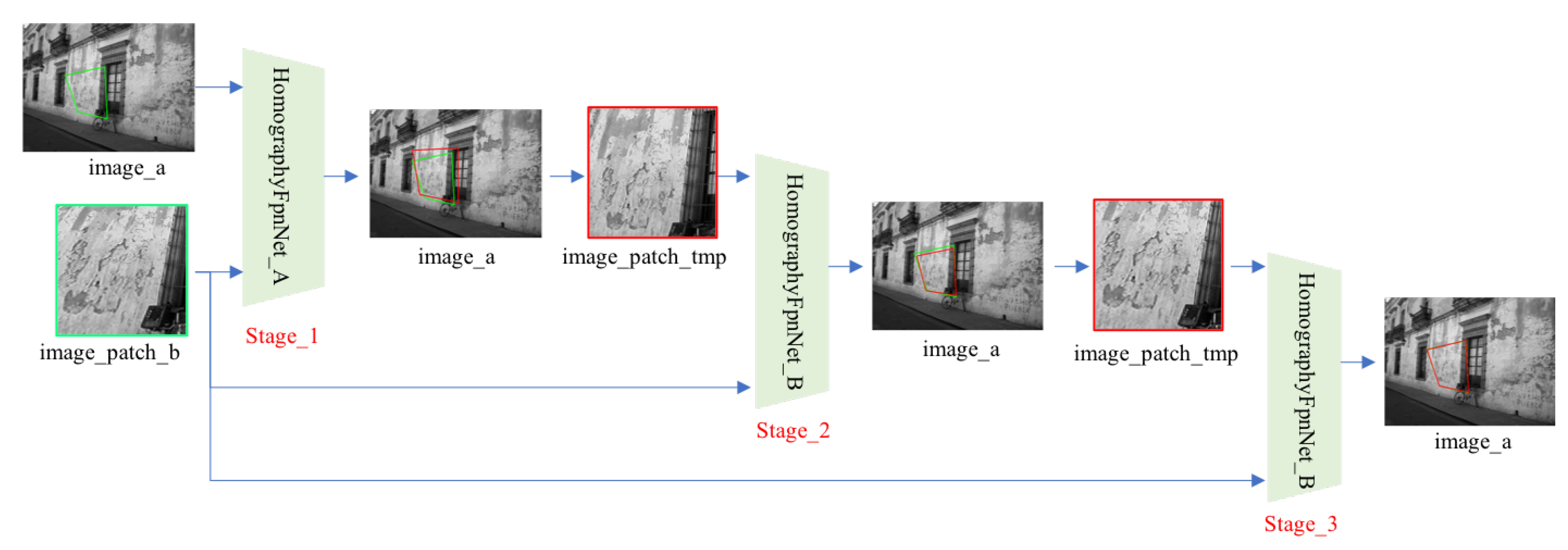
4.2. Hierarchical Homography Estimation

To predict the four-point homography values, the locations of the four corners of image_patch_b were predicted in image_a. To successively reduce the estimation error, we used a hierarchical method, as shown in Figure 7.

In Stage_1, we took the input image pair of image_a and image_patch_b and used the HomographyFpnNet_A model to directly predict the pixel coordinates of the four corners of image_patch_b in image_a. The training triplet sample of Stage_1 was (image_a, image_patch_b, $p_j$), j = 0, 1, 2, 3. In the following Stage_i (i = 2, 3), we first used the prediction result of the preceding stage (Stage_i − 1) to calculate the homography matrix $H_{i-1}$ between image_a and image_patch_b, and then used $H_{i-1}$ to transform the area enclosed by the predicted four corners of Stage_i-1 in image_a (red quadrilaterals in Figure 7) to a new image_patch_tmp of size $128\times 128$ pixels. At the same time, we used $H_{i-1}$ to transform the ground truth four-point homography values to image_patch_tmp to provide target regression values for Stage_i. We then took the input image pair of image_patch_tmp and image_patch_b and used the HomographyFpnNet_B model to predict the pixel offsets of the four corners of image_patch_b in image_patch_tmp relative to the four corners of image_patch_tmp. Finally, we used the inverse of $H_{i-1}$ to transform the predicted four corners of HomographyFpnNet_B back to image_a to get the predicted four corners of image_patch_b in the original image_a for Stage_i. The training triplet sample of stage_i was (image_patch_tmp, image_patch_b, $H_{i-1}{p}_j$), j = 0, 1, 2, 3.

The model structures of HomographyFpnNet_A and HomographyFpnNet_B are exactly the same as that shown in Figure 3. The difference between HomographyFpnNet_A and HomographyFpnNet_B is that, while the output of HomographyFpnNet_A represents the absolute pixel values of the four corners of image_patch_b in image_a, the output of HomographyFpnNet_B represents the pixel offsets of the four corners of image_patch_b in image_patch_tmp relative to the four corners of image_patch_tmp.

Warping using the predicted four-point homography values from each stage (red quadrilaterals in Figure 7) resulted in a more visually similar image_patch_tmp to image_patch_b, as shown in Figure 7. We took the predicted four-point homography values of the last stage as our final result.

4.3. Training

As shown in Figure 7, when training the hierarchical models, the training data of the current stage model depended on the predictions from the previous stage model. When training the three cascade models at the same time, we needed to do some data processing, such as warping image_a to generate image_patch_tmp, in real time, which resulted in a slow training speed. To speed up the training, we adopted a step-by-step training strategy and prepared training data for each stage model offline.

Firstly, the training set generated by the method shown in Figure 6 was taken as Training Set 1 to train the Stage_1 model (a HomographyFpnNet_A model). Secondly, we used the predictions of the trained Stage_1 model to generate Training Set 2 offline, and then Training Set 2 was used to train the Stage_2 model (a HomographyFpnNet_B model). Thirdly, predictions from the trained Stage_2 model were used to generate Training Set 3 offline, and then Training Set 3 was used to train the Stage_3 model (also a HomographyRegNet_B model).

For simplicity, we used the same training parameters or the training of all stage models (i.e., one HomographyFpnNet_A model and two HomographyFpnNet_B models). For the training of each stage model, we used the same training parameters and methods as for the center-aligned image pair case, except that we used 130,000 training iterations rather than 90,000. During the training process, we also adopted the following data enhancement strategies for the image pairs. For image_patch_b (size of $128\times 128$ pixels) in the image pair, we randomly adjusted its brightness and assigned random values to a randomly chosen small rectangle (size: $w\times h,4\le w\le 16,4\le h\le 16$). The main reason for using these two data enhancement strategies was to avoid issues that arise when the wall maps are used, such as illumination changes between the camera image and the wall map, the occlusion of the camera images by the robot, and so on. We used these data enhancement strategies to improve the estimation accuracy of the trained hierarchical HomographyFpnNet model on the test wall images.

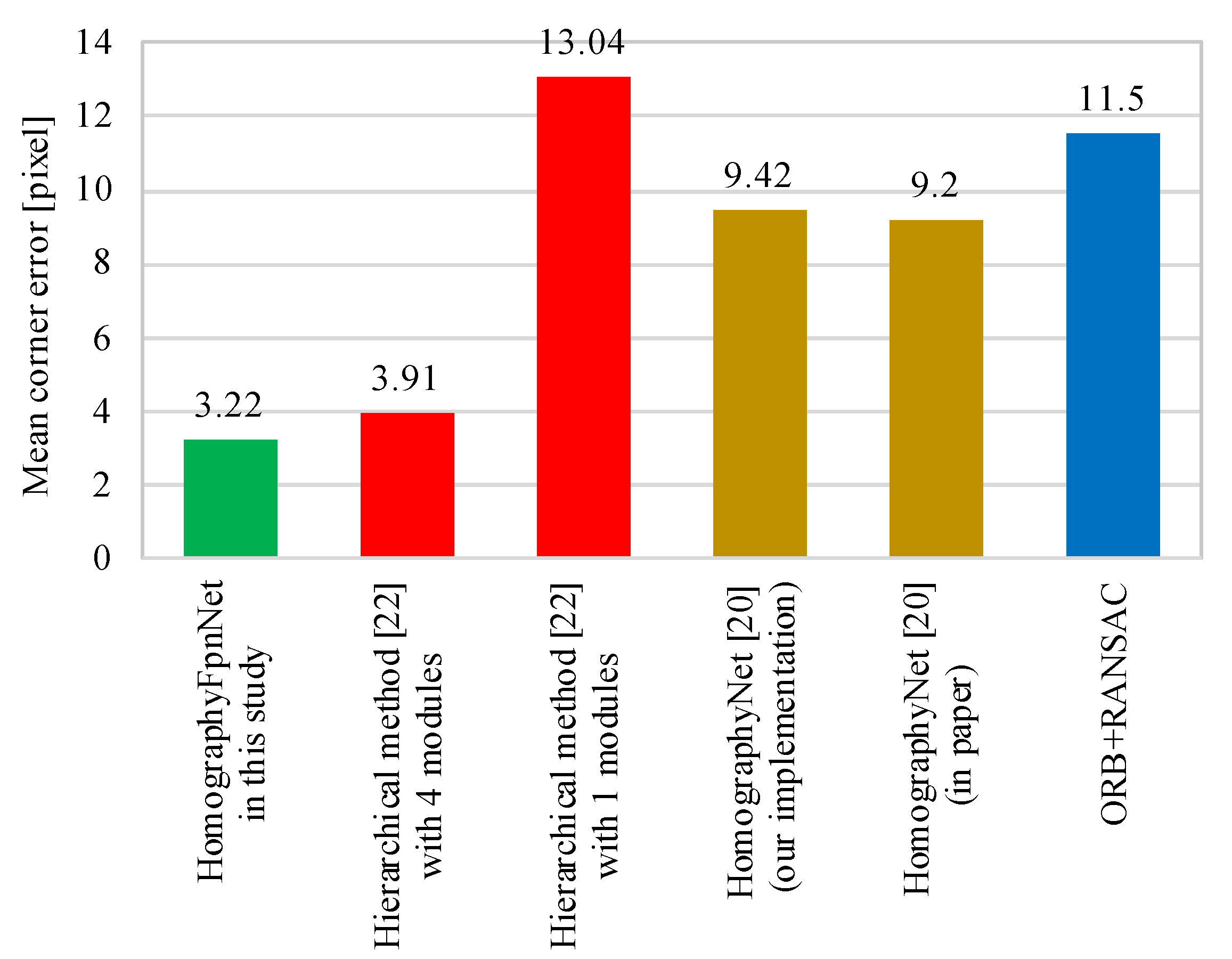
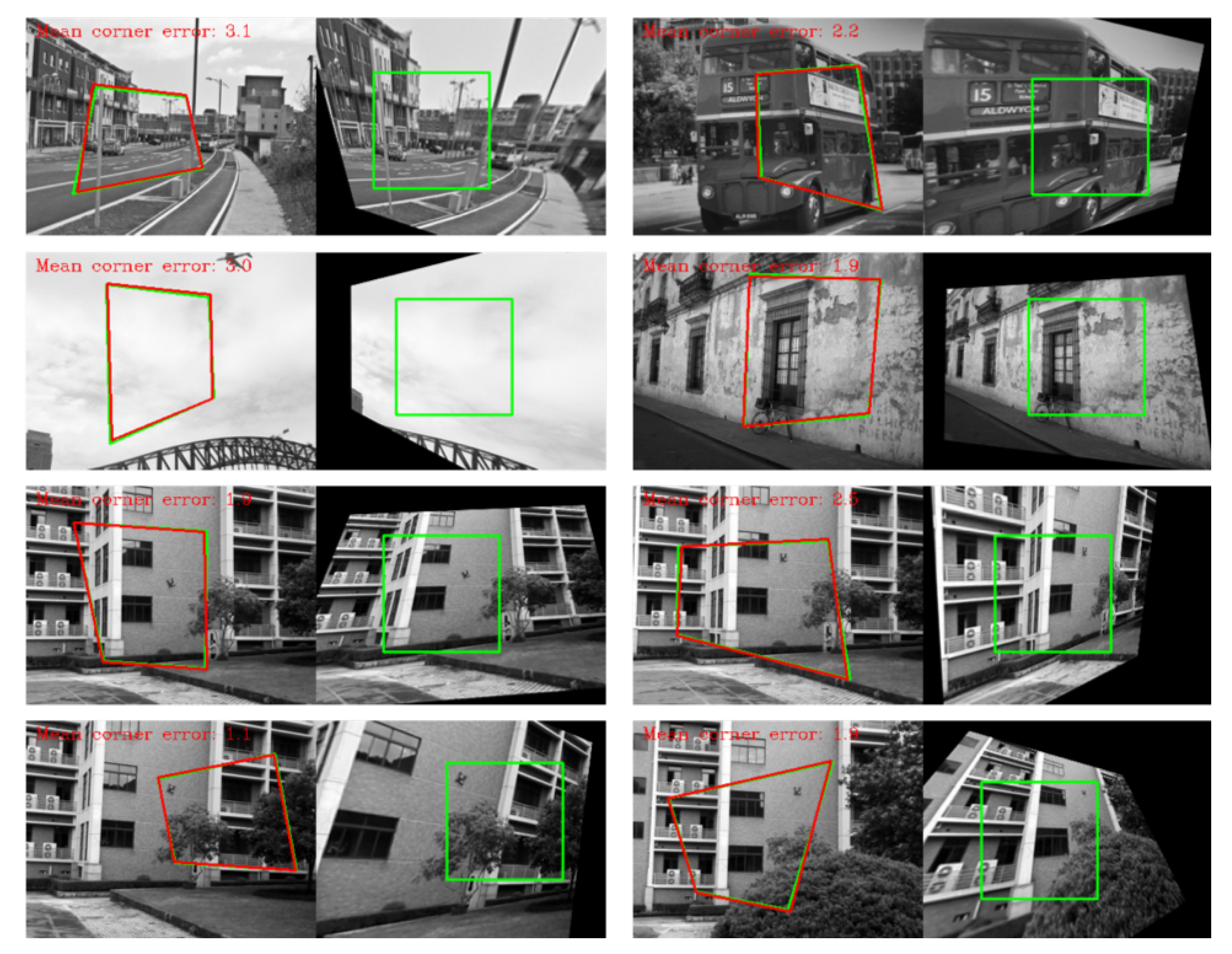
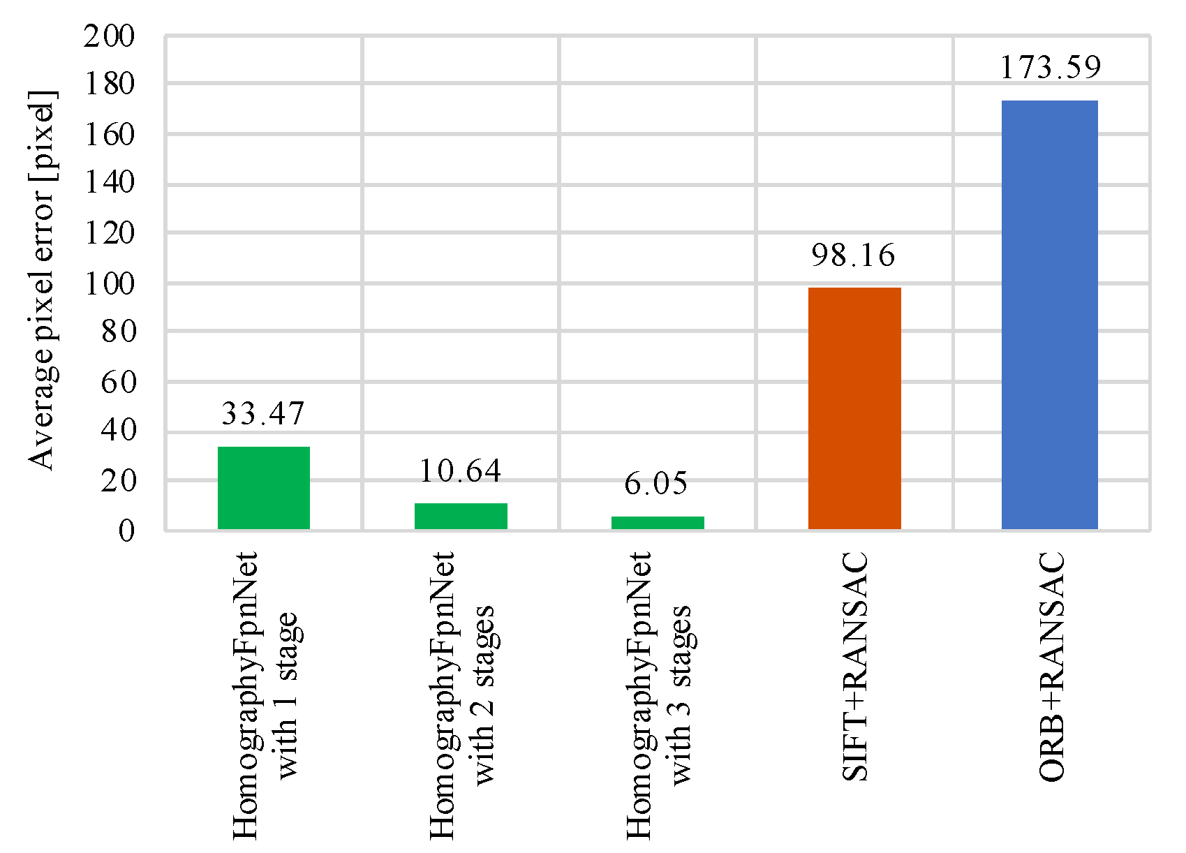
4.4. Results and Discussion

We compared our hierarchical HomographyFpnNet with the baseline of classical ORB/SIFT+RANSAC methods for homography estimation of non-center-aligned image pairs. We report the metric of mean corner error for each approach on the 30,000 test samples generated from the MS-COCO 2014 test set. To measure this metric, we computed the L2 distance between the ground truth corner position and the estimated corner position in the original image_a. In other words, for hierarchical HomographyFpnNet, we first resized image_a to a size of $128\times 128$ pixels for the prediction, and then we resized the predicted corners back to the original image_a size to compute the error in the corner positions. The error was averaged over the four corners of the image, and the mean corner error was computed over the entire test set (30,000 samples). We used the default OpenCV parameters in the traditional ORB/SIFT+RANSAC homography estimator, which computes ORB/SIFT features at multiple scales and uses the top 25 scoring matches as input to the RANSAC estimator. To avoid extremely large corner error, the estimated four-point homography values of ORB/SIFT+RANSAC method were clipped within the shape size of image_a. In scenarios where the ORB/SIFT+RANSAC estimate failed, we ignored the estimate and excluded that test sample.

As shown in Figure 8, the ORB+RANSAC method performed poorly in the homography estimation of non-center-aligned image pairs, with a mean corner error of 173.59 pixels. The method of SIFT+RANSAC performed better and obtained a mean corner error of 98.16 pixels, while the detection speed of SIFT features was much slower than that of ORB features. The reason that ORB/SIFT+RANSAC methods performed poorly in the homography estimation of non-center-aligned image pairs is that the size of image_patch_b is smaller than image_a, causing many mismatches of ORB/SIFT feature points between image_a and image_patch_b. Our hierarchical HomographyFpnNet performed much better in this task, and the mean corner error of the three-stage model was only 6.05 pixels. Figure 9 shows some prediction results obtained with our three-stage hierarchical HomographyFpnNet method compared with those obtained with ORB/SIFT+RANSAC methods, in which the corners of the green boxes are ground truth four-point homography values and the corners of the red boxes are predicted results.

4.5. Time Consumption Analysis

We used Tensorflow [26] to implement our proposed network model. During testing, the average processing time of a single HomographyFpnNet model on a GPU was 3.48 ms. Using the HomographyFpnNet model in each stage of the hierarchical method, the total computational complexity is given by,

$$d_e=(l_m+l_w)\ast n$$

(1)

where $d_e$ is the end-to-end delay of the whole hierarchical model, $l_m$ is the average latency for each HomographyFpnNet model, $l_w$ is the warping over-head to prepare a new image pair, and n is the number of stages used in the hierarchical model.

Table 1. Time consumption of our hierarchical HomographyFpnNet.

Model Name	Time Consumption on a GPU (ms)
One-stage hierarchical HomographyFpnNet	3.48
Two-stage hierarchical HomographyFpnNet	7.03
Three-stage hierarchical HomographyFpnNet	10.8

shows the time consumption of our hierarchical HomographyFpnNet model on a GPU. Our three-stage hierarchical HomographyFpnNet model is shown to have an average processing time of 10.8 ms on a GPU. The real-time processing speed satisfies the requirements of wall-climbing robots.

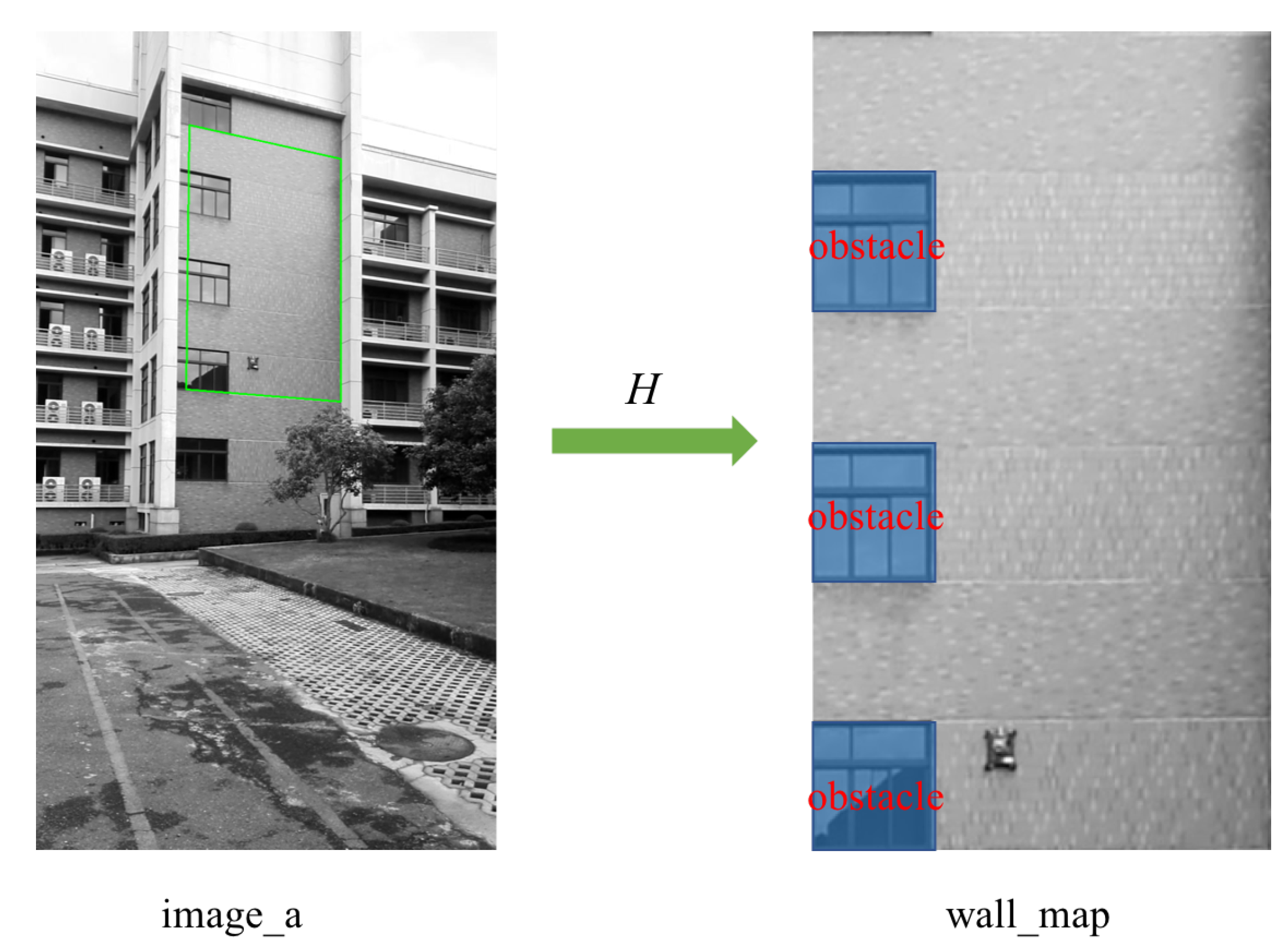
5. Experiment on Wall Images

We conducted a homography estimation on the wall images of our wall-climbing robots using the previously trained three-stage hierarchical HomographyFpnNet model. The test wall images were decoded from the recorded video (one image per 2 s) and there were 52 images ($1280\times 720$ pixels) in total. We selected four fixed points on the wall and manually labeled the pixel coordinates of these four fixed points on each wall image. After conducting the four-point homography prediction with our three-stage HomographyFpnNet model, we resized the predicted four-point values back to the original image size, and then calculated the mean corner error; the mean corner error was computed in the image size of $1280\times 720$ pixels.

In the first experiment, for each image_a of wall image, we first warped the labeled four-point homography values (green box in Figure 10) to get image_patch_b, and then used the trained three-stage hierarchical HomographyFpnNet model and the input image pair (image_a, image_patch_b) to predict the four-point homography values (red box in Figure 10). The four-point homography estimation errors of our three-stage HomographyFpnNet on the 52 test wall images are shown in Figure 11, and the mean corner error of the 52 images was only 2.8 pixels. Figure 10 shows some prediction results on the wall images.

In the second experiment, we conducted a more difficult test. We used a single image_patch_b generated from the first wall image to estimate the four-point homography values between this image_patch_b and all test wall images. Experiment 2 was consistent with the actual use of the wall map of the wall-climbing robot. That is, we usually prepared one wall map image and then estimated the four-point homography between the wall map and all camera images. As can be seen in Figure 12, while the matched region of image_a is occluded by the wall-climbing robot, even though there is no robot in the corresponding image_patch_b, our model could still estimate the four-point homography values well due to the data enhancement strategy we used when training the hierarchical HomographyFpnNet model (described in th e Section 3.3). Figure 13 shows the prediction error when using a single image_patch_b, with a mean corner error of the 52 test wall images of 5.1 pixels. The mean corner error of 5.1 pixels in the second experiment was larger than the 2.2 pixels in the first experiment, and this increased error was mainly caused by the difference between the image_a and the fixed image_patch_b increasing over time. This is a problem that we will solve in the future, for example generating training samples of fixed image_patch_b and a changeable image_a from videos.

6. Conclusions

We proposed HomographyFpnNet, which uses multi-scale deep visual features, and obtained a smaller homography estimation error for center-aligned image pairs compared with the state of the art. The proposed hierarchical HomographyFpnNet for non-center-aligned image pairs significantly outperforms ORB/SIFT+ RANSAC methods. The experiments conducted with a trained three-stage hierarchical HomographyFpnNet model on wall images of climbing robots showed that our proposed hierarchical HomographyFpnNet is suitable for estimating the homography matrix between the wall map and camera images. In future work, we will focus on solving the problem of increasing estimation error of homography caused by the change in illumination, viewpoint, etc. between the camera image and the fixed wall map.

References

1. Armada, M.; Prieto, M.; Akinfiev, T.; Fernandez, R.; González, P.; García, E.; Montes Coto, H.J.; Nabulsi, S.; Ponticelli, R.; Sarria, J.; et al. On the design and development of climbing and walking robots for the maritime industries. J. Marit. Res. 2005, 2, 9–31. [Google Scholar]
2. Armada, M.; de Santos, P.G. Climbing, walking and intervention robots. Ind. Robot Int. J. 1997, 24, 158–163. [Google Scholar] [CrossRef]
3. Akinfiev, T.; Armada, M.; Nabulsi, S. Climbing cleaning robot for vertical surfaces. Ind. Robot Int. J. 2009, 36, 352–357. [Google Scholar] [CrossRef]
4. Zhou, Q.; Li, X. Experimental comparison of drag-wiper and roller-wiper glass-cleaning robots. Ind. Robot Int. J. 2016, 43, 409–420. [Google Scholar] [CrossRef]
5. Kim, T.Y.; Kim, J.H.; Seo, K.C.; Kim, H.M.; Lee, G.U.; Kim, J.W.; Kim, H.S. Design and Control of a Cleaning Unit for a Novel Wall-Climbing Robot. Appl. Mech. Mater. 2014, 541–542, 1092–1096. [Google Scholar] [CrossRef]
6. Huang, H.; Li, D.; Xue, Z.; Chen, X.; Liu, S.; Leng, J.; Wei, Y. Design and performance analysis of a tracked wall-climbing robot for ship inspection in shipbuilding. Ocean Eng. 2017, 131, 224–230. [Google Scholar] [CrossRef]
7. Sayab, M.; Aerden, D.; Paananen, M.; Saarela, P. Virtual Structural Analysis of Jokisivu Open Pit Using `Structure-from-Motion’ Unmanned Aerial Vehicles (UAV) Photogrammetry: Implications for Structurally-Controlled Gold Deposits in Southwest Finland. Remote Sens. 2018, 10, 1296. [Google Scholar] [CrossRef]
8. Arai, Y.; Sekiai, M. Absolute position measurement system for mobile robot based on incident angle detection of infrared light. In Proceedings of the 2003 IEEE/RSJ International Conference on Intelligent Robots and Systems (IROS 2003) (Cat. No.03CH37453), Las Vegas, NV, USA, 27–31 October 2003. [Google Scholar]
9. Yan, C.; Zhan, Q. Real-time multiple mobile robots visual detection system. Sens. Rev. 2011, 31, 228–238. [Google Scholar] [CrossRef]
10. Wang, C.; Fu, Z. A new way to detect the position and orientation of the wheeled mobile robot on the image plane. In Proceedings of the 2014 IEEE International Conference on Robotics and Biomimetics (ROBIO 2014), Bali, Indonesia, 5–10 December 2014. [Google Scholar]
11. Lowe, D.G. Distinctive Image Features from Scale-Invariant Keypoints. Int. J. Comput. Vis. 2004, 60, 91–110. [Google Scholar] [CrossRef]
12. Rublee, E.; Rabaud, V.; Konolige, K.; Bradski, G. ORB: An efficient alternative to SIFT or SURF. In Proceedings of the 2011 International Conference on Computer Vision, Barcelona, Spain, 6–13 November 2011. [Google Scholar]
13. Fischler, M.A.; Bolles, R.C. Random sample consensus: A paradigm for model fitting with applications to image analysis and automated cartography. Commun. ACM 1981, 24, 381–395. [Google Scholar] [CrossRef]
14. Badrinarayanan, V.; Kendall, A.; Cipolla, R. SegNet: A Deep Convolutional Encoder-Decoder Architecture for Image Segmentation. IEEE Trans. Pattern Anal. Mach. Intell. 2017, 39, 2481–2495. [Google Scholar] [CrossRef] [PubMed]
15. He, K.; Gkioxari, G.; Dollár, P.; Girshick, R. Mask R-CNN. In Proceedings of the IEEE International Conference on Computer Vision, Venice, Italy, 22–29 October 2017. [Google Scholar]
16. Cao, Z.; Hidalgo, G.; Simon, T.; Wei, S.E.; Sheikh, Y. OpenPose: Realtime Multi-Person 2D Pose Estimation using Part Affinity Fields. In Proceedings of the IEEE Conference on Computer Vision and Pattern Recognition, Honolulu, HI, USA, 21–26 July 2017. [Google Scholar]
17. Mikolov, T.; Chen, K.; Corrado, G.; Dean, J. Efficient Estimation of Word Representations in Vector Space. arXiv 2013, arXiv:1301.3781. [Google Scholar]
18. Fischer, P.; Dosovitskiy, A.; Ilg, E.; Häusser, P.; Hazırbaş, C.; Golkov, V.; van der Smagt, P.; Cremers, D.; Brox, T. FlowNet: Learning Optical Flow with Convolutional Networks. arXiv 2015, arXiv:1504.06852. [Google Scholar]
19. Ilg, E.; Mayer, N.; Saikia, T.; Keuper, M.; Dosovitskiy, A.; Brox, T. FlowNet 2.0: Evolution of Optical Flow Estimation with Deep Networks. In Proceedings of the IEEE Conference on Computer Vision and Pattern Recognition, Las Vegas, NV, USA, 27–30 June 2016. [Google Scholar]
20. DeTone, D.; Malisiewicz, T.; Rabinovich, A. Deep Image Homography Estimation. arXiv 2016, arXiv:1606.03798. [Google Scholar]
21. Simonyan, K.; Zisserman, A. Very Deep Convolutional Networks for Large-Scale Image Recognition. arXiv 2014, arXiv:1409.1556. [Google Scholar]
22. Nowruzi, F.E.; Laganiere, R.; Japkowicz, N. Homography Estimation from Image Pairs with Hierarchical Convolutional Networks. In Proceedings of the 2017 IEEE International Conference on Computer Vision Workshops, Venice, Italy, 22–29 October 2017. [Google Scholar]
23. Lin, T.-Y.; Maire, M.; Belongie, S.; Hays, J.; Perona, P.; Ramanan, D.; Dollár, P.; Zitnick, C. Lawrence Microsoft COCO: Common Objects in Context. In Proceedings of the European Conference on Computer Vision, Zurich, Switzerland, 6–12 September 2014. [Google Scholar]
24. Lin, T.Y.; Dollár, P.; Girshick, R.; He, K.; Hariharan, B.; Belongie, S. Feature Pyramid Networks for Object Detection. In Proceedings of the IEEE Conference on Computer Vision and Pattern Recognition, Las Vegas, NV, USA, 27–30 June 2016. [Google Scholar]
25. Loshchilov, I.; Hutter, F. SGDR: Stochastic Gradient Descent with Warm Restarts. arXiv 2016, arXiv:1608.03983. [Google Scholar]
26. Abadi, M.; Agarwal, A.; Barham, P.; Brevdo, E.; Chen, Z.; Citro, C.; Corrado, G.S.; Davis, A.; Dean, J.; Devin, M.; et al. TensorFlow: Large-Scale Machine Learning on Heterogeneous Distributed Systems. arXiv 2016, arXiv:1603.04467. [Google Scholar]
Figure 1. Projection transformation from camera image to wall map using homography matrix H: (Left) original camera image, denoted as image_a; and (Right) wall map (front view of the wall), corresponding to the green quadrilateral in image_a.
Applsci 09 02908 g001
Figure 2. Center-aligned and non-center-aligned image pairs. image_patch_a is the rectangle crop of image_a around the ground truth green quadrilateral, and image_patch_b is the warping of the ground truth green quadrilateral.
Applsci 09 02908 g002
Figure 3. Structure of HomographyFpnNet.
Applsci 09 02908 g003
Figure 4. Mean corner pixel error comparison of various methods for homography estimation of a center-aligned image pair.
Applsci 09 02908 g004
Figure 5. HomographyFpnNet results on test images. The corners of the green quadrilaterals are the ground truth and the corners of the red quadrilaterals are the predicted results.
Applsci 09 02908 g005
Figure 6. Dataset generation of a non-center-aligned image pair.
Applsci 09 02908 g006
Figure 7. Estimation process of the hierarchical HomographyFpnNet model. The four corners of the green quadrilateral in image_a are the ground truth four-point homography values; the four corners of the red quadrilateral in image_a are the predicted results.
Applsci 09 02908 g007
Figure 8. Test error comparison of our hierarchical HomographyFpnNet with other methods for non-center-aligned image pairs. Pixel errors are all computed in the original image_a size.
Applsci 09 02908 g008
Figure 9. Homography estimation results of different methods for non-center-aligned image pair. The corners of green box are ground truth four-point homography values and the corners of red box are predicted results.
Applsci 09 02908 g009
Figure 10. Experiment 1. Prediction results of our three-stage hierarchical HomographyFpnNet on test wall images where image_patch_b is warped from each wall image. The corners of the green box are the ground truth four-point homography values and the corners of the red box are the predicted results. Since the error of the homography estimation is very small, the red and green boxes almost overlap.
Applsci 09 02908 g010
Figure 11. Experiment 1. Prediction errors of our three-stage hierarchical HomographyFpnNet on test wall images.
Applsci 09 02908 g011
Figure 12. Experiment 2. Prediction results of our three-stage hierarchical HomographyFpnNet on test wall images where image_patch_b is only warped from the first wall image.
Applsci 09 02908 g012
Figure 13. Experiment 2. Prediction errors of our three-stage hierarchical HomographyFpnNet on test wall images.
Applsci 09 02908 g013