Artificial Neural Network for Vertical Displacement Prediction of a Bridge from Strains (Part 1): Girder Bridge under Moving Vehicles

Abstract

A real-time prediction method using a multilayer feedforward neural network is proposed for estimating vertical dynamic displacements of a bridge from the longitudinal strains of the bridge when vehicles pass across it. A numerical model for an existing five-girder bridge spanning 36 m proved by actual experimental values was used to verify the proposed method. To obtain a realistic vehicle distribution for the bridge, vehicle type and actual headways of moving vehicles were taken, and the measured vehicle distribution was generalized using Pearson Type III theory. Twenty-five load scenarios were created with assumed vehicle speeds of 40 km/h, 60 km/h, and 80 km/h. The results indicate that the model can reasonably predict the overall displacements of the bridge (which is difficult to measure) from the strain (which is relatively easy to measure) in the field in real time.

1. Introduction

Bridges are a critical infrastructure that are used for the movement of goods and people, so the evaluation of their safety is very important. The real-time evaluation of the safety of such structures is called structural health monitoring (SHM). Through SHM, it is possible to quickly address urgent situations, such as the threat of collapse. In addition to extending the life of a structure, SHM can reduce its maintenance costs [1]. SHM can be divided into two categories: safety evaluation to assess the load bearing capacity of a structure and serviceability evaluation to assess the degree of deformation present [2]. In SHM, various physical data are collected. Of these, data on the displacement of structures constitute one of the most basic data types, useful in evaluating both safety and serviceability [2,3]. From the displacements of a structure, the behavior and strength of a structure can be intuitively confirmed. In addition, by observing its long-term displacement history, the degree of deterioration and degree of damage suffered by a structure can be clearly ascertained. For these reasons, many studies have been conducted on methods of measuring the displacements of a structure [1,2,3,4,5,6,7].

Methods for measuring the displacements of a structure can be generally classified as contact or non-contact measurements [1,8,9]. Devices for contact-type measurements include linear variable differential transformers (LVDTs) and cable-type displacement transducers. These contact-type devices generally have a very high accuracy [1]. However, these devices are affected by the installation site because they require contact with the structure. For example, it is very difficult to install equipment for bridges that have very high clearance, such as bridges in valleys or bridges over rivers or oceans. Non-contact devices include laser, radar, GPS, and video or digital cameras [1] and many methods to measure displacement using non-contact devices have been studied [10,11,12,13,14,15,16,17,18,19]. These devices are guaranteed to be accurate within 1 mm owing to advances in technology. However, they usually need complex computer algorithms and are affected by environmental factors such as light. Furthermore, although existing equipment can measure the displacement of a structure at a given time, it is limited in its ability to continuously measure the displacement of a structure in real time.

In addition to methods for directly measuring the displacement of a structure, there are studies for estimating displacement using strain and acceleration, which are relatively easy to measure [20,21,22,23,24,25,26]. According to Euler–Bernoulli beam theory, displacement can be calculated by integrating the strain; however, there are limitations in applying theoretical behavior to actual structures. The displacement can also be obtained by integrating the acceleration twice. When using the boundary condition to obtain the integral constant, an error occurs because the boundary condition of the actual structure does not match the theory.

In this study, an artificial neural network (ANN) was used as an alternative to overcome the limitations of the above displacement estimation method. An ANN is a computer algorithm that simulates the human central nervous system, and ANNs have a strong ability to capture correlations between two variables that are difficult to formulate or have a very complex relationship [27]. An ANN can justify the correlation between the two variables by learning rather than by using conventional mathematical formulas. Due to these advantages, The ANN was used to predict displacements. In general, it is very difficult to define the relationship between longitudinal strain and vertical displacement analytically in a complex real structure. However, using the data mapping capability of ANN, the relationship between strain and displacement can be clearly defined after the training process. Therefore, it is possible to predict the displacement of the structure in real-time with only strain data that is relatively easy to measure in the field. Also, if training is done properly, the displacement of the structure can be predicted quickly and accurately without any extra cost. Because of their capabilities, many studies on data prediction using ANNs have been conducted in various fields [27,28,29,30,31,32,33,34,35,36,37,38,39,40].

In this paper, a method for real-time prediction of the overall vertical displacement distribution of a structure is proposed—particularly, a bridge—from measurements of longitudinal strain, which is relatively easy to measure, using the advantages of ANN. For the training of the ANN, training data was acquired from a finite element model (FEM) verified with experimental values as an alternative to collecting hard-to-obtain actual data. Also, by using various numbers of hidden layers and nodes, the prediction accuracy of ANN by ANN structures was compared.

2. Methodology

In this study, a method of predicting displacements using ANN from strains, which is relatively easy to measure, is proposed. Training data (strains, displacements) is obtained from the verified FEM model. For testing the trained ANN, strains measured from sensors installed on the actual structure should be input to the trained ANN to compare the predicted displacements with the measure displacements. However, since the purpose of this paper is to propose a displacements prediction method, the test data was also obtained from the FEM. The proposed displacements method is demonstrated in the next section.

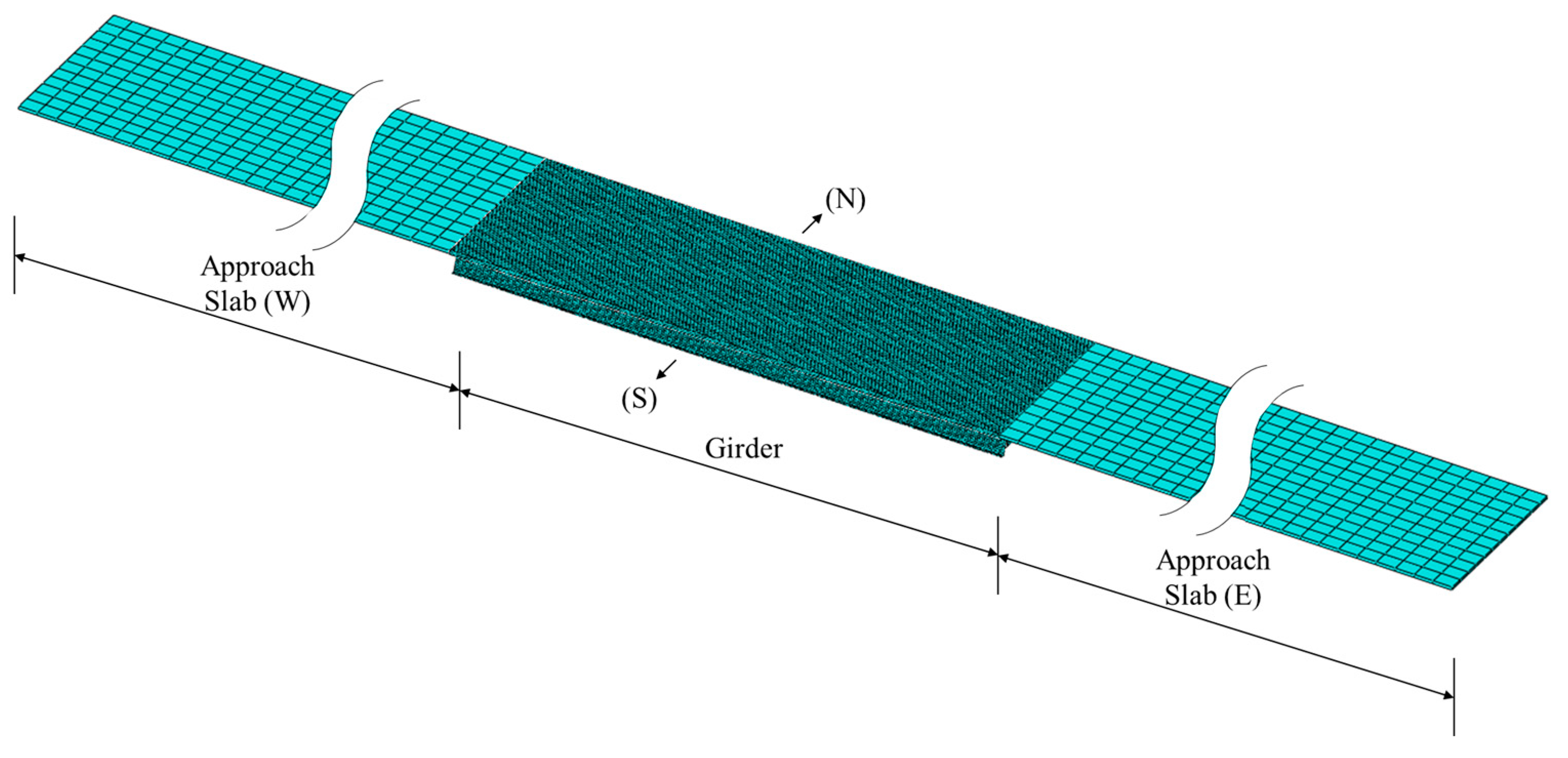
2.1. Numerical Model

In this study, a finite element model (FEM) was used to obtain training and test data for the ANN. If measured data are available, a more realistic prediction will be possible, but as mentioned in Section 1, measuring displacement is not easy. The motivation for this study is developing another method to predict displacement. Therefore, an FEM verified with experimental values was used as an alternative. It is assumed that the results analyzed from the verified FEM correspond to the actual data. In order to carry out the finite element analysis (FEA), a simple supported slab-and-girder bridge was selected. The span of the slab was set to 36 m and the width of the slab to 15 m (Figure 1a). It is assumed that the bridge carried four lanes of traffic, two in each direction. I-shaped steel girders were used (Figure 1b). The unit weight of the concrete slab is 2300 kgf/m³ and the modulus of elasticity is 30 GPa. Also, the unit weight of the steel girder is 8000 kgf/m³ and the modulus of elasticity is 200 GPa. For the loads applied to the bridge, only the vehicle load was considered. Dynamic analysis was performed assuming that all materials are within the elastic range and are homogeneous and isotropic. The commercial program ABAQUS for FEM was used. Three-dimensional solid elements were used for the bottom slab of the bridge, and three-dimensional shell elements were used for the girders. In order to analyze the dynamic behavior due to the passing of the vehicle load over the bridge, it is modeled as shown in Figure 2. At both ends of the bridge, approach portions were modeled to minimize any numerical problems that might occur between the bridge and the entrance as a vehicle moved onto the bridge. The numerical model used was verified by comparing it to experimental values under static and dynamic loads [41,42,43].

The behavior of bridges is affected by these factors, such as vehicle weight, length, suspension, and natural period. Because these interfere with each other in a complex manner, it is difficult to construct a model that considers all variables. Therefore, in this study, it is assumed that the vehicles are limited to three types—passenger cars, buses, and trucks—and that they move at constant speeds. The dynamic performance of structures can be affected by various factors such as loading type, geometry, and so on [44]. In this paper, the dynamic interaction between the bridge and the moving vehicles can have relevant effects. To express these interactions, FE model based on the vehicle model proposed by Zuo and Nayfeh [44] was used. The vehicle model includes the mass, spring, and damper which have different dynamic behavior with bridge. The specifications of the models used for cars, buses, and trucks were used those proposed by Zuo and Nayfeh [45], Ahmed et al. [46], and Li [47].

2.2. Data Collection

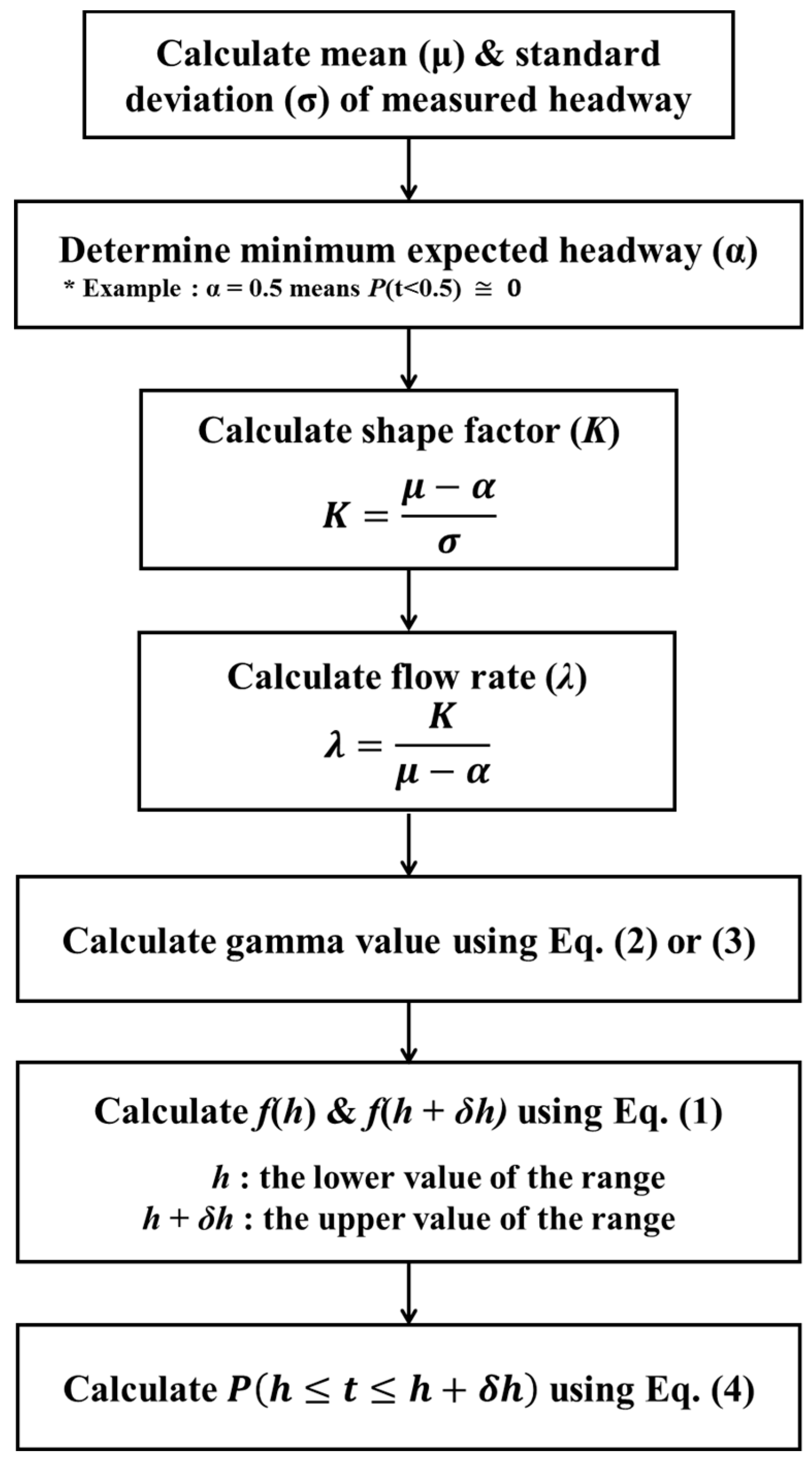
2.2.1. Pearson Type III Distribution

In order to describe the distribution of the vehicles as near to the actual situation as possible when loading the vehicle data into the FEM, a camera was installed in a fixed position in front of the starting point of the actual bridge for measuring (Figure 3), and the actual vehicle types and headways (i.e., interval times) were collected. Although the FEM used in this study and the actual bridge for measuring are not identical, it is assumed that it does not have a significant effect on the prediction result since the measured data was applied to Pearson Type III distribution, a probabilistic theory of general traffic flow. The vehicle types are assumed to be passenger cars, buses, or trucks.

Table 1. Number (percentage) of each vehicle type for each lane during the measurement period (20 min).

	Cars (%)	Buses (%)	Trucks (%)	Total
Lane 1	248 (91.51)	17 (6.27)	6 (2.22)	271
Lane 2	350 (92.59)	27 (7.14)	1 (0.27)	378
Lane 3	223 (84.47)	41 (15.53)	0 (0)	264
Lane 4	174 (94.05)	7 (3.78)	4 (2.17)	185

shows the measured results by lane.

Statistics were also introduced to generalize the measured headway values of the vehicles. The traffic situation was generalized using Pearson Type III theory assuming the most general intermediate flow of traffic [48]. Pearson Type III theory is a generalized function of the gamma distribution and is often used to describe traffic conditions [49]. The Pearson Type III probability density function at arbitrary headway t is given by Equation (1).

$$f\left(t\right)=\frac{\lambda }{\Gamma \left(K\right)}{\left[\lambda \left(t-\alpha \right)\right]}^{K-1}{e}^{-\lambda \left(t-\alpha \right)}$$

(1)

where λ is the flow rate and can be calculated using the mean value (μ) of the measured headway, α, and K; α is the minimum expected headway; and K is the shape factor that can be calculated using μ, α, and the standard deviation (σ) of the measured headway. Γ is the gamma function and is defined as

$$\Gamma \left(K\right)=\left(K-1\right)!$$

(2)

If K is not an integer, the gamma function can be calculated numerically as

$$\Gamma \left(K\right)={{\displaystyle \int }}_0^{\infty }{e}^{-x}{x}^{K-1}dx$$

(3)

Using the probability density function (Equation (1)), the probability (P) that any headway (t) is between h and h + δh can be estimated numerically as

$$P\left(h\le t\le h+\delta h\right)={{\displaystyle \int }}_h^{\infty }f\left(t\right)dt-{{\displaystyle \int }}_{h+\delta h}^{\infty }f\left(t\right)dt\approx \left[\frac{f\left(h\right)+f\left(h+\delta h\right)}{2}\right]\times \delta h$$

(4)

To apply Pearson Type III theory to the measured headway, seven steps are required, as given in Figure 4.

Figure 5 shows the observed headway and the headway generalized using Pearson Type III theory. As seen in the figure, the observed headway shows some differences from the generalized headway because it has characteristics specific to a particular area. Nevertheless, it can be seen that the distribution of the headway generalized by applying Pearson Type III theory represents the measured headway distribution well overall.

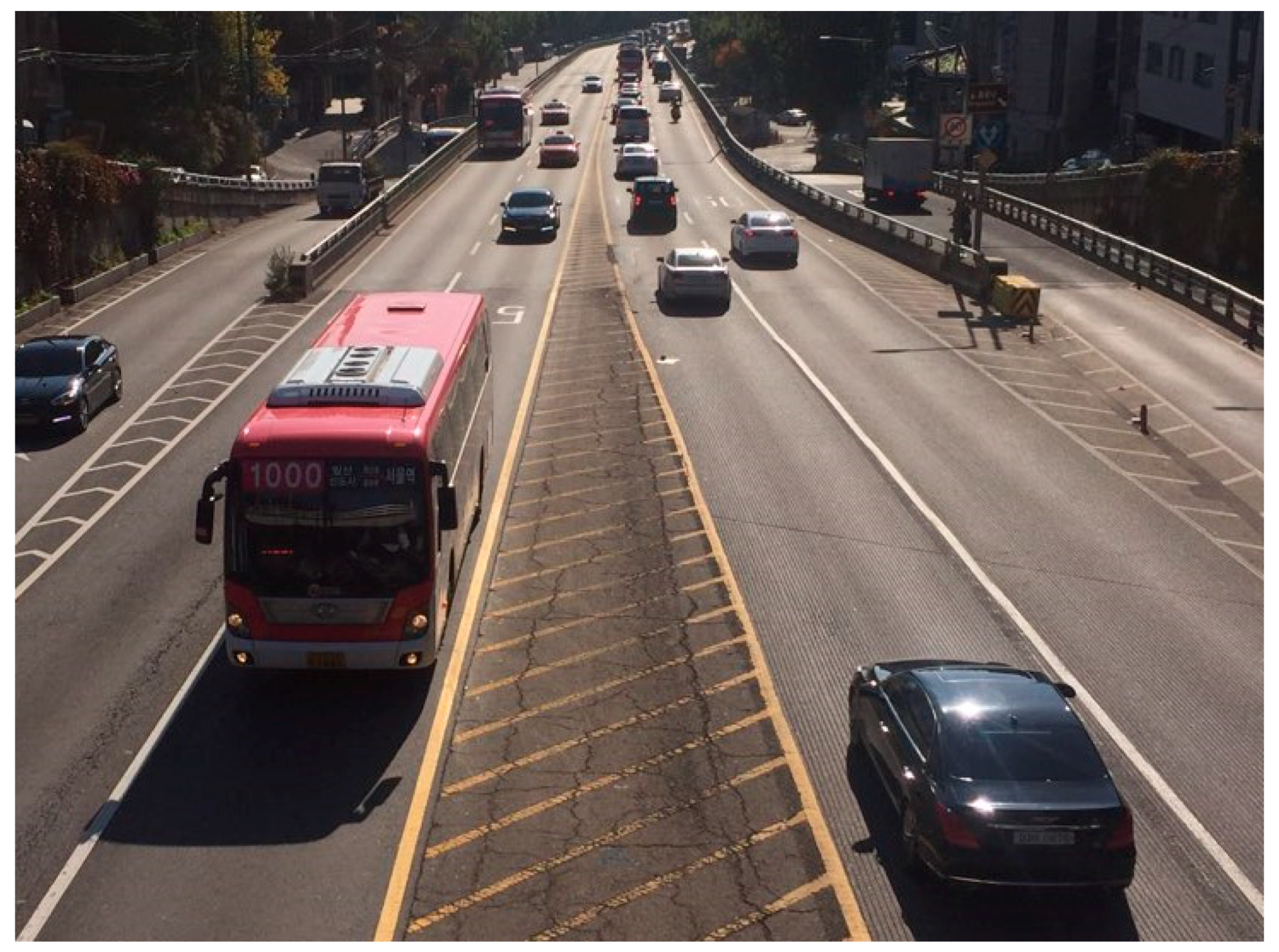
2.2.2. Load Scenarios

In order to create the load scenarios for the FEA, the proportions of the vehicle types in Table 1 and the headways in Figure 5 was used. It is created an algorithm that selects a vehicle type for each lane with the proportions in Table 1, and at the same time, sets the headway of the vehicle to the probability shown in Figure 5. The headway is multiplied by the speed to calculate the distance between the vehicles. For each of three speeds (40 km/h, 60 km/h, and 80 km/h), 25 load scenarios were created using the algorithm. Figure 6 shows one example of the vehicle distribution scenario for 60 km/h.

2.2.3. Data Collection

The load scenarios created as described in Section 2.2.2 were loaded into the FEM, and FEA was performed. Strains and displacement measurements were obtained at 11 locations at uniform intervals of 3.6 m below the flange of each girder, as shown in Figure 7. The center point is included as a measurement point because the largest displacement generally occurs at the center of the girder. Both ends of the beam were included to confirm that the strain and displacement at the support points in the simple supported beam are zero. Thus, a total of 55 strain (11 points × 5 girders, input) and displacement (11 points × 5 girders, output) measurement points were set. That is, one data set contains 55 strains and 55 displacements. The FEA for 25 scenarios for each speed was performed using the load scenarios created as described in Section 2.2.2. The value of Δt was 0.01 s, and the vehicles were loaded for a total of 8 s so that many vehicles could completely pass across the bridge. Thus, 800 data sets per scenario was obtained.

Table 2. Number of training and test data sets.

	Training Data			Test Data
	40 km/h	60 km/h	80 km/h	40 km/h	60 km/h	80 km/h
Number of load scenarios	24	24	24	1	1	1
Number of data sets per scenario	800	800	800	800	800	800
Total number of data sets	24 $\times$ 800 $\times$ 3 = 57,600			1 $\times$ 800 $\times$ 3 = 2400

One data set consists of 55 strains (input) and 55 displacements (output).

shows the amounts of training and test data obtained.

An ANN is significantly less predictive of data beyond the range of the data that were used for training. In other words, if the range of data to be predicted is outside the range of data used for training, the prediction accuracy of the ANN is lowered. Therefore, the range of the test data should be configured to be within the range of the training data [27]. In this study, one scenario was selected such that the strain and displacement values used in the testing for each speed were within the range of values used in the training, as shown in

Table 3. Ranges of strain and displacement values.

Girder		Training Data		Test Data
		Min.	Max.	Min.	Max.
Longitudinal Strain (=input)	S2	−1.9485 × 10−5	20.1969 × 10−5	−4.1586 × 10−6	4.0053 × 10−5
	S1	−1.4692 × 10−5	12.5891 × 10−5	−4.3175 × 10−6	5.3966 × 10−5
	CG	−0.7784 × 10−5	9.0571 × 10−5	−4.7890 × 10−6	4.3134 × 10−5
	N1	−0.7014 × 10−5	9.5812 × 10−5	−2.9181 × 10−6	2.5414 × 10−5
	N2	−2.6651 × 10−5	16.3720 × 10−5	−3.4250 × 10−6	1.5924 × 10−5
Vertical Displacement (=output, unit: mm)	S2	−16.0033	1.0827	−3.4275	0.4020
	S1	−10.2574	0.5583	−3.4660	0.2214
	CG	−6.6549	0.4138	−2.9460	0.2268
	N1	−7.8640	0.5330	−2.1045	0.2295
	N2	−12.0705	2.4387	−1.2924	0.2450

. A total of 57,600 data sets were used as training data, and a total of 2400 data sets were used as test data, with 800 data sets per speed. In general, the quantity of data used for training should be greater than the quantity of data used in the test [34]. The difference between the quantity of training data and test data in this study is considered to be appropriate.

2.3. Multilayer Feedforward Neural Network (MFNN)

ANNs are computer algorithms that simulate human central nervous system information processing. When a human brain receives information, it is processed in the central nervous system and a final decision is made. The nervous system is made up of cells called neurons, and ANNs have neuron-like nodes. ANNs have a special ability to define the correlation of data in nonlinear relationships [33]. The neural network, first introduced by McCulloch and Pitts [50], has since been developed into various types of network models. Among these, the most efficient and widely used model is the multilayer feedforward neural network (MFNN) [51]. The structure of a general MFNN assuming the number of hidden nodes is J is shown in Figure 8. As shown in the figure, the MFNN consists of an input layer for inputting data, a hidden layer for computing with the input data, and an output layer for predicting the target value. Each layer consists of many nodes. The nodes of each layer are mathematically connected to the nodes of adjacent layers (input layer–hidden layer, hidden layer–output layer). Weights are assigned to the connections between layers. In addition, a bias is assigned to each node of the hidden layer and the output layer. In order for the ANN to accurately predict the target value, the optimal weight and bias should be determined, which is done through training. The process of training an artificial neural network is as follows.

First, training data must be prepared for the learning process. These training data consist of input (I) and target output (T) values. In this study, 55 strain values were used as input values and 55 displacement values as output values. The prepared input values are used in a calculation along with the first weight and bias generated randomly, and the calculated values are input to the hidden layer

$$net\_hidde{n}_j={\displaystyle \sum }_{i=1}^{55}{w}_{ij}{I}_i+{\theta }_j$$

(5)

where $I_i$ is the variable input to the $i$th node of the input layer, $w_{ij}$ is the weight assigned between the $i$th node of the input layer and the $j$th node of the hidden layer, and ${\theta }_j$ is the bias assigned to the $j$th node of the hidden layer. The result, $net\_hidde{n}_j$, is the weighted sum of all input variables and the bias and is input to the $j$th node of the hidden layer. The value $net\_hidde{n}_j$ input to the hidden layer is calculated through the transfer function

$$Z_j=f\left(net\_hidde{n}_j\right)$$

(6)

where $f$ is the transfer function in the hidden layer, and $Z_j$ is the output value of the $j$th node of the hidden layer calculated through the transfer function and the variable input to the output layer. The same process is applied between the hidden layer and the output layer. The error is calculated by comparing the predicted output (K) with the target output (T) of the training data (feedforward). If the computed error does not satisfy the user-defined criteria, the ANN goes back to the hidden layer and the input layer and corrects the weight and bias using the training algorithm (backward) [52]. Through this iterative process, the error between the predicted output (K) and the target output (T) is reduced. If the criteria set by the user are met, the training stops and the optimal weights and biases have been determined.

2.4. Modeling of MFNN

The predictive power of ANNs depends heavily on its architecture. In general, the architecture of an MFNN is defined by four elements [53]: number of layers, number of nodes in each layer, type of transfer function in each layer, and type of training function.

Recently, many studies have been undertaken to optimize ANN architecture [53]. However, there is still no scientific method or general rule for finding the optimal architecture of an ANN [34]. Therefore, in this study, the architecture of the ANN was determined through a case study, which is the technique generally followed [34]. The four elements as applied in the case study method are as follows.

• The numbers of input layers and output layers are both fixed at one. Therefore, regarding the total number of layers, the number of hidden layers is the only variable. In general, as the number of hidden layers increases, the computational speed decreases proportionately, and the learning efficiency decreases because of the large amount of computer memory required. With consideration of these points, in this research, the case study was conducted with the number of hidden layers limited to two.
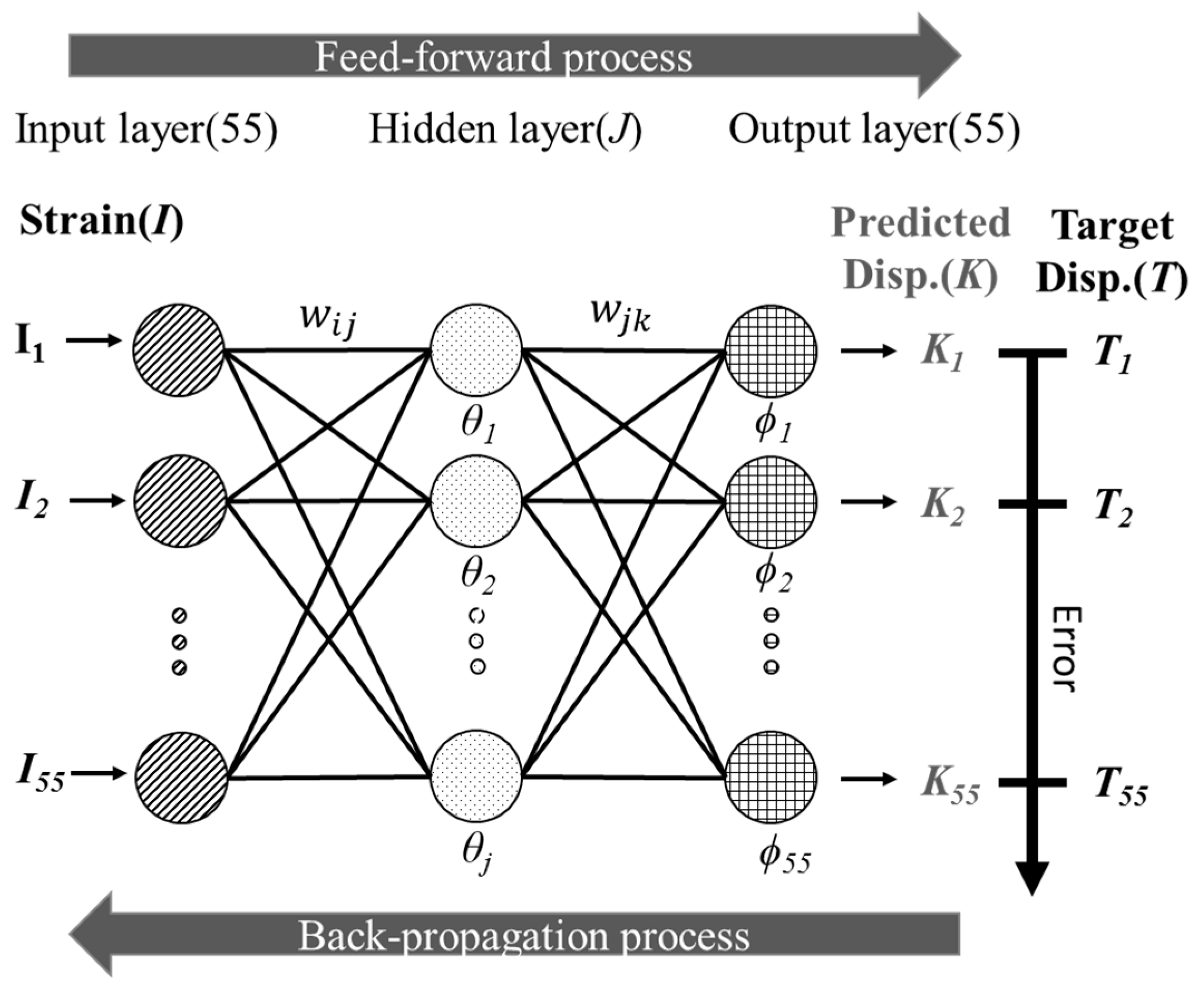
• The number of nodes in the input layer and the output layer is already determined because it is equal to the number of variables that are input and output, respectively, for the problem to be studied [54]. Therefore, the number of nodes in hidden layer is the only variable. There are no general rules for setting the number of hidden nodes [53]. The number of nodes proposed by Zhang et al. was used [55]. In their study, they proposed n/2, n, 2n, and 2n + 1 for the number of hidden nodes, where n is the number of input nodes. In this study, as the number of nodes in the input layer is 55, 28 (n/2), 55 (n), 110 (2n), and 111 (2n + 1) was used as the number of nodes in the hidden layer.
• The transfer function transforms the weighted sum of the input values to the output node and determines the strength of the output value [56]. Nalbant et al. [57] asserted that the transfer function is determined by the nature of the problem to be solved. In this study, a log-sigmoid function (logsig) was used for the hidden layer and a linear function (purelin) for the output layer, which is a commonly used transfer function [33].
• The training function determines the method of calculating the error of the predicted output value and adjusts the weight and bias. The training function is important because it can considerably affect the learning speed and accuracy [53]. The training function is affected by many factors, such as the nature of the problem, amount of data, and the number of weights. That is, even for a given function, the accuracy and the learning time may vary depending on the nature of the problem. In this study, a relatively large quantity of data (57,600) was used for learning. Therefore, trainscg was used as the learning function, which has relatively low memory consumption and low time consumption, as well as high accuracy when there are many data [58].

The above parameters are shown in

Table 4. General information for the artificial neural network (ANN) model.

Number of input nodes (strain values)	55
Number of hidden layers	1 or 2
Number of hidden nodes	28, 55, 110, or 111
Number of output nodes (displacement values)	55
Number of training data	57,600
Number of test data	2400 (800 + 800 + 800)
Training algorithm	Scaled conjugate gradient backpropagation
Transfer function	Logsig (hidden), Purelin (output)
Learning rate	0.01
Momentum	0.9

. With two cases for the number of hidden layers and four cases for the number of nodes in the hidden layers, a total of eight cases were created for the ANN architecture (no. of input nodes-no. of first hidden nodes (-no. of second hidden nodes)–no. of output nodes): 55-28-55, 55-28-28-55, 55-55-55, 55-55-55-55, 55-110-55, 55-110-110-55, 55-111-55, and 55-111-111-55. The log-sigmoid function is set in the hidden layer and the pure linear function in the output layer. The scaled conjugate gradient backpropagation algorithm was used for training. A total of eight case studies were conducted to evaluate the accuracy of the neural network architecture.

3. Results and Discussion

In this section, the training accuracy of the ANN by the various numbers of hidden layers and nodes is compared using the training data obtained, as described in Section 2.2.3 and the parameters presented in Section 2.4. In addition, it is examined the test results according to the architecture of the ANN and compared the displacements at a certain point over time and the displacement distribution at a certain time.

3.1. Training Results by ANN Structure

A MATLAB R2018a toolbox was used to train the artificial neural network. At the beginning of training, initial weights, and biases are generated randomly, so different training results can be obtained for the same structure [59]. In this study, a total of 20 training sessions were performed with each structure, and the average training results are shown in

Table 5. Training results by ANN structure.

Case	No. of Hidden Layers	ANN Structure	Training Performance		Training Time (s)
			MSE (×10−3)	R
1	1	55-28-55	1.31	0.998728	840.30
2		55-55-55	1.20	0.998829	1566.92
3		55-110-55	1.10	0.998927	3403.87
4		55-111-55	1.10	0.998928	3440.74
5	2	55-28-28-55	1.83	0.998225	997.67
6		55-55-55-55	1.48	0.998556	3544.24
7		55-110-110-55	1.28	0.998753	16,852.07
8		55-111-111-55	1.30	0.998734	15,442.72

MSE, mean squared error; R, correlation coefficient.

and Figure 9. The mean squared error (MSE) was used as the training performance function; it is the one most commonly used in MFNN [60]. The mean squared error (MSE) is given by

$$MSE=\frac{1}{N}{\displaystyle \sum }_{i=1}^N{(T_i-K_i)}^2$$

(7)

In Equation (7), T is the target output and K is the predicted output. The closer the MSE is to zero, the smaller the error. As the MSE is affected by the absolute magnitude of the output (displacements), there is a limit to judging training performance by MSE only. Therefore, use of the correlation coefficient (R) value is suggested, and the correlation between the predicted value and the actual value is presented. The closer R is to 1, the higher the prediction accuracy. The training times for each ANN structure are presented in Table 5. From this table, two features can be found. First, the prediction accuracy varies according to the number of hidden layers and the number of nodes in the hidden layer(s). When there was one hidden layer, the minimum and maximum MSE values were 0.001103 (case 4) and 0.001308 (case 1), respectively. The minimum and maximum R values were 0.998728 (case 1) and 0.998928 (case 4), respectively. When there were two hidden layers, the minimum and maximum MSE values were 0.001282 (case 7) and 0.001825 (case 5), respectively. The minimum and maximum R values were 0.998225 (case 5) and 0.998753 (case 7), respectively. From Figure 9, it can be seen that the effect of the ANN architecture on MSE is similar to that on the R value. In general, the greater the number of hidden layers and nodes, the higher the prediction accuracy. However, as the number continues to increase, the accuracy may decrease because of overtraining. In this study, the learning accuracy was higher in the cases of one hidden layer than in the cases of two hidden layers. It is also seen that for a given number of hidden layers, the greater the number of nodes, the higher the prediction accuracy. The second feature found in Table 5 is that the training time varies according to the number of hidden layers and the number of nodes. For cases 1, 2, 3, and 4, the training time was 840.30 s, 1566.92 s, 3403.87 s, and 3440.74 s, respectively. In case 1, the number of hidden nodes was 28, and in case 2, the number of hidden nodes was 55, which is about twice that for case 1, and the training time was also about twice that for case 1. Similarly, the number of hidden nodes for case 3 was twice as large as that for case 2, and the learning time was also about twice that for case 2. For cases 3 and 4, the number of hidden nodes was similar, so there was no notable difference in training time. For cases 5, 6, 7, and 8, the training time was 997.67 s, 3544.24 s, 16,852.07 s, and 15,442.72 s, respectively. In case 5, the number of hidden-layer nodes was 28, and in case 6, the number of hidden-layer nodes was 55, which is about twice that for case 5, and the number of hidden layers was 2. As a result, the training times differed by a factor of about 3.5. For cases 6 and 7, the number of hidden-layer nodes differed by a factor of 2, and the number of hidden layers was 2. As a result, the training times differed by a factor of about 4.7. From these results, it can be seen that the ANN training time is proportional to the number of nodes in the hidden layer(s), but the effect is larger when the number of hidden layers is two.

In general, the number of hidden layers and nodes is the most influential factor in ANN training [34]. However, in this study, it can be confirmed that the learning ability of the ANN is not substantially affected by the number of hidden layers and nodes. In other words, it is considered that, despite the differences among the network structures, fairly high accuracy is shown for all of the ANN structures.

3.2. Test Results by ANN Structure

For the ANN trained with eight different structures having various numbers of hidden layers and nodes, testing was performed using data that were not used for training. The purpose of the test is to determine whether overfitting has occurred during the training process. Overfitting refers to situations in which the ANN is trained well, but the trained ANN do not predict data well. This means that the ANN simply memorized the correlation between the input and output values of the training data rather than defining it well [60]. This is an important process because in order to be practically applicable, an ANN must be able to produce accurate predictions for untrained data.

The test procedure was as follows. The strain obtained from the analysis of a load scenario that was not used for training was input to the ANN trained as described in Section 3.1. The trained ANN can predict displacement (output) immediately, which is one of the advantages of ANN. Then, the displacement predicted by the ANN was compared with the displacement obtained from the analysis. The data used in this test were those for the one load scenario for each of the three velocities (40 km/h, 60 km/h, and 80 km/h) that were not used for training, as mentioned in Section 2.2.3. All ANN architectures trained as described in Section 3.1 were tested, and the test results were reviewed. For testing, as the output value is immediately predicted after the input is entered into the trained neural network, the training time is not indicated separately. The test results are shown in

Table 6. Test results by ANN structure.

Case	No. of Hidden Layers	ANN Structure	Velocity of Vehicles Crossing Bridge (Test)
			40 km/h		60 km/h		80 km/h
			MSE (×10−3)	R	MSE (×10−3)	R	MSE (×10−3)	R
1	1	55-28-55	0.70	0.995533	0.37	0.996351	0.44	0.993415
2		55-55-55	0.68	0.995636	0.35	0.996528	0.43	0.993614
3		55-110-55	0.67	0.995699	0.34	0.996641	0.42	0.993773
4		55-111-55	0.67	0.995705	0.34	0.996645	0.42	0.993755
5	2	55-28-28-55	0.77	0.995058	0.45	0.995594	0.50	0.992507
6		55-55-55-55	0.74	0.995256	0.41	0.995997	0.46	0.993179
7		55-110-110-55	0.70	0.995498	0.38	0.996296	0.44	0.993502
8		55-111-111-55	0.70	0.995519	0.38	0.996282	0.44	0.993464

, and the error for the load scenario at 40 km/h is shown in Figure 10. From the results for 40 km/h, when there was one hidden layer, the minimum and maximum MSE values were 0.67 × 10⁻³ (case 4) and 0.70 × 10⁻³ (case 1), respectively. The minimum and maximum R values were 0.995533 (case 1) and 0.995705 (case 4), respectively. When there were two hidden layers, the minimum and maximum MSE values were 0.70 × 10⁻³ (case 8) and 0.77 × 10⁻³ (case 5), respectively. The minimum and maximum R values were 0.995058 (case 5) and 0.995519 (case 8), respectively. Compared to the training results, the accuracy rankings for the structures with 110 and 111 hidden layers differed. However, as the difference is very small, it is considered that the test results are similar to the training results. Similar results were obtained for 60 km/h and 80 km/h. The test MSE values for 40 km/h and 60 km/h are smaller than the training MSE values, and the test MSE values for 80 km/h are larger than the training MSE values. This is because the MSE is affected by the magnitude of the absolute value. In addition, a comparison of the R values shows that the R value in testing was smaller than that for training for all velocities. Therefore, it is considered that the test results are slightly reduced in accuracy compared to the training results. However, we can see fairly good test results for MSE and R overall. Particularly in the cases with one hidden layer, a higher accuracy is shown. Therefore, it can be confirmed that the ANN was not overfitting, indicating that training and testing progressed very well.

The test results for the case of 55-111-55 (case 4), which showed the highest accuracy among the various ANN architectures, are shown in Figure 11, Figure 12, Figure 13 and Figure 14. Figure 11, Figure 12 and Figure 13 show the dynamic displacement over time for the midpoint, where the largest displacement is expected to occur. Figure 14 shows the overall behavior of the bridge at the time of maximum displacement for each speed. The following observations are made from the graphs.

• The ANN trained using three different velocities predicts the displacement for different speed–load scenarios with remarkably high accuracy. This means that it is possible to predict the displacement of a bridge due to a vehicle moving at various velocities in the field.
• The ANN predicts the overall behavior of all the girders at a given point in time, as well as the change in dynamic displacement of a given point over time.
• The results provide that the proposed method to predict vertical dynamic displacements of bridge from longitudinal strains is feasible.

$$\mathrm{Difference}=\left|\mathrm{Disp}\_\mathrm{FEM}-\mathrm{Disp}\_\mathrm{ANN}\right|$$

(8)

4. Conclusions and Future Work

In this study, a method to predict the vertical displacement (output) of bridges was proposed from the longitudinal strain (input) generated when vehicles pass across bridges by using an ANN. Pearson Type III distribution theory was used to express the actual vehicle distribution, and the training and test data were acquired using the verified FEM as an alternative to the difficulty of obtaining actual data. The proposed method showed the predictability of a bridge’s dynamic displacement, which is relatively difficult to measure. ANN, which has a strong ability to define correlations between data, and a verified FEM for training data were used to predict displacement from strain, which is relatively easy to measure. Displacement is one of the most important types of physical data in the SHM of bridges. In addition, ANN can continuously predict displacement in real time. By using the proposed method, it is expected that the prediction of displacement of bridges and other structures, whether in use or newly constructed, can become easier and economically feasible.

It is also examined the prediction accuracy by ANN structure, which has the greatest influence on the general prediction accuracy of an ANN. The comparison of the prediction accuracy for various numbers of hidden layers and of nodes suggested by Zhang et al. [55] showed a fairly high accuracy for all structures. Although the structure of the ANN does not have a major influence on the prediction accuracy in this study and it is costly and time consuming to find an ANN structure that has high accuracy, it is considered to be one of the processes that the researcher must perform to achieve better prediction.

In the present study, the feasibility of displacement prediction by ANN is confirmed using an FE bridge model, not the real bridge. In future work, an experiment to apply the proposed method to actual bridge will be conducted. Especially, with actual bridges, natural conditions such as temperature and wind load may cause noise to the measured strains and displacements. Future study is intended to quantify the relation between the prediction accuracy and noise by predicting the displacements using measured data with noise. Also, study on determining the minimum number of strain-measurement points required for predicting displacements will be conducted using optimization techniques such as genetic algorithm.

References

1. Ribeiro, D.; Calçada, R.; Ferreira, J.; Martins, T. Non-contact measurement of the dynamic displacement of railway bridges using an advanced video-based system. Eng. Struct. 2014, 75, 164–180. [Google Scholar] [CrossRef]
2. Park, S.W.; Park, H.S.; Kim, J.H.; Adeli, H. 3D displacement measurement model for health monitoring of structures using a motion capture system. Measurement 2015, 59, 352–362. [Google Scholar] [CrossRef]
3. Zhao, X.; Liu, H.; Yu, Y.; Xu, X.; Hu, W.; Li, M.; Ou, J. Bridge displacement monitoring method based on laser projection-sensing technology. Sensors 2015, 15, 8444–8463. [Google Scholar] [CrossRef] [PubMed]
4. Feng, D.; Feng, M.Q. Vision-based multipoint displacement measurement for structural health monitoring. Struct. Control Health Monit. 2016, 23, 876–890. [Google Scholar] [CrossRef]
5. Huang, Q.; Crosetto, M.; Monserrat, O.; Crippa, B. Displacement monitoring and modelling of a high-speed railway bridge using C-band Sentinel-1 data. ISPRS J. Photogramm. Remote Sens. 2017, 128, 204–211. [Google Scholar] [CrossRef]
6. Sekiya, H.; Kimura, K.; Miki, C. Technique for determining bridge displacement response using MEMS accelerometers. Sensors 2016, 16, 257. [Google Scholar] [CrossRef] [PubMed]
7. Vicente, M.A.; Gonzalez, D.C.; Minguez, J.; Schumacher, T. A novel laser and video-based displacement transducer to monitor bridge deflections. Sensors 2018, 18, 970. [Google Scholar] [CrossRef]
8. Lee, J.J.; Cho, S.; Shinozuka, M.; Yun, C.-B.; Lee, C.-G.; Lee, W.-T. Evaluation of bridge load carrying capacity based on dynamic displacement measurement using real-time image processing techniques. Steel Struct. 2006, 6, 377–385. [Google Scholar]
9. Lee, J.J.; Fukuda, Y.; Shinozuka, M.; Cho, S.; Yun, C.-B. Development and application of a vision-based displacement measurement system for structural health monitoring of civil structures. Smart Struct. Syst. 2007, 3, 373–384. [Google Scholar] [CrossRef]
10. Olaszek, P. Investigation of the dynamic characteristics of bridge structures using a computer vision method. Measurement 1999, 25, 227–236. [Google Scholar] [CrossRef]
11. Nakamura, S. GPS measurement of wind-induced suspension bridge girder displacements. J. Struct. Eng. 2000, 126, 1413–1419. [Google Scholar] [CrossRef]
12. Brown, C.; Roertsm, G.; Meng, X. When bridges move: GPS-based deflection monitoring. Sensors 2006, 4, 16–19. [Google Scholar]
13. Lee, J.; Shinozuka, M. A vision-based system for remote sensing of bridge displacement. Ndt E Int. 2006, 39, 425–431. [Google Scholar] [CrossRef]
14. Gonzalez-Aguilera, D.; Gomez-Lahoz, J.; Sanchez, J. A new approach for structural monitoring of large dams with a three-dimensional laser scanner. Sensors 2008, 8, 5866–5883. [Google Scholar] [CrossRef]
15. Fukuda, Y.; Feng, M.; Shinosuka, M. Cost-effective vision-based system for monitoring dynamic response of civil engineering structures. Struct. Control Health Monit. 2009, 17, 918–936. [Google Scholar] [CrossRef]
16. Park, J.W.; Lee, J.J.; Jung, H.J.; Myung, H. Vision-based displacement measurement method for high-rise building structures using partitioning approach. Ndt E Int. 2010, 43, 642–647. [Google Scholar] [CrossRef]
17. Im, S.B.; Hurlebaus, S.; Kang, Y.J. Summary Review of GPS technology for structural health monitoring. J. Struct. Eng. 2013, 139, 1653–1664. [Google Scholar] [CrossRef]
18. Kohut, P.; Holak, K.; Uhl, T.; Ortyl, L.; Owerko, T.; Kuras, P.; Kocierz, R. Monitoring of a civil structure’s state based on noncontact measurements. Struct. Health Monit. 2013, 12, 411–429. [Google Scholar] [CrossRef]
19. Psimoulis, P.A.; Stiros, S.C. Measuring deflections for a short-span railway bridge using a robotic total station. J. Bridge Eng. 2013, 18, 182–185. [Google Scholar] [CrossRef]
20. Li, C.J.; Ulsoy, A.G. High-precision measurement of tool-tip displacement using strain gauges in precision flexible line boring. Mech. Syst. Signal. Proc. 1999, 13, 531–546. [Google Scholar] [CrossRef]
21. Kang, L.H.; Kim, D.K.; Han, J.H. Estimation of dynamic structural displacements using fiber Bragg grating strains sensors. J. Sound. Vib. 2007, 305, 534–542. [Google Scholar] [CrossRef]
22. Tommy, H.T.C.; Demeke, B.A.; Tam, H.Y. Vertical displacement measurements for bridges using optical fiber sensors and CCD cameras-a preliminary study. Struct. Health. Monit. 2009, 8, 243–249. [Google Scholar]
23. Wang, Z.C.; Geng, D.; Ren, W.X. Strain modes based dynamic displacement estimation of beam structures with strain sensors. Smart. Mater. Struct. 2014, 23, 125045. [Google Scholar] [CrossRef]
24. Xia, Y.; Zhang, P.; Ni, Y.Q. Deformation monitoring of a super-tall structure using real-time strain data. Eng. Struct. 2014, 67, 29–38. [Google Scholar] [CrossRef] [Green Version]
25. Xu, H.; Ren, W.X.; Wang, Z.C. Deflection estimation of bending beam structures using fiber Bragg grating strain sensors. Adv. Struct. Eng. 2015, 18, 395–404. [Google Scholar] [CrossRef]
26. Cho, S.; Yun, C.B.; Sim, S.H. Displacement estimation of bridge structure using data fusion of acceleration and strain measurement incorporating finite element model. Smart. Struct. Syst. 2015, 15, 645–663. [Google Scholar] [CrossRef]
27. Chandwani, V.; Agrawal, V.; Nagar, R. Modeling slump of ready mix concrete using genetic algorithms assisted training of Artificial Neural Networks. Expert Syst. Appl. 2015, 42, 885–893. [Google Scholar] [CrossRef]
28. Hamzehie, M.E.; Mazinani, S.; Davardoost, F.; Mokhtare, A.; Najibi, H.; Van der Bruggen, B.; Darvishmanesh, S. Developing a feed forward multilayer neural network model for prediction of CO2 solubility in blended aqueous amine solutions. J. Nat. Gas Sci. Eng. 2014, 21, 19–25. [Google Scholar] [CrossRef]
29. Hemmat Esfe, M.; Hassani Ahangar, M.R.; Rejvani, M.; Toghraie, D.; Hajmohammad, M.H. Designing an artificial neural network to predict dynamic viscosity of aqueous nanofluid of TiO2 using experimental data. Int. Commun. Heat Mass Transf. 2016, 75, 192–196. [Google Scholar] [CrossRef]
30. Ostad-Ali-Askari, K.; Shayannejad, M.; Ghorbanizadeh-Kharazi, H. Artificial neural network for modeling nitrate pollution of groundwater in marginal area of Zayandeh-rood River, Isfahan, Iran. KSCE J. Civ. Eng. 2017, 21, 134–140. [Google Scholar] [CrossRef]
31. Ramasamy, P.; Chandel, S.S.; Yadav, A.K. Wind speed prediction in the mountainous region of India using an artificial neural network model. Renew. Energy 2015, 80, 338–347. [Google Scholar] [CrossRef]
32. Yadav, A.K.; Chandel, S.S. Solar radiation prediction using Artificial Neural Network techniques: A review. Renew. Sustain. Energy Rev. 2014, 33, 772–781. [Google Scholar] [CrossRef]
33. Yan, F.; Lin, L.; Wang, X.; Azarmi, F.; Sobolev, K. Evaluation and prediction of bond strength of GFRP-bar reinforced concrete using artificial neural network optimized with genetic algorithm. Compos. Struct. 2017, 161, 441–452. [Google Scholar] [CrossRef]
34. Zain, A.M.; Haron, H.; Sharif, S. Prediction of surface roughness in the end milling machining using Artificial Neural Network. Expert Syst. Appl. 2010, 37, 1755–1768. [Google Scholar] [CrossRef]
35. Elsheikh, A.H.; Showaib, E.A.; Asar, A.E.M. Artificial neural network based forward kinematics solution for planar parallel manipulators passing through singular configuration. Adv. Robot. Autom. 2013, 2, 2. [Google Scholar]
36. Karabacak, K.; Cetin, N. Artificial neural networks for controlling wind-PV power systems: A review. Renew. Sustain. Energy Rev. 2014, 29, 804–827. [Google Scholar] [CrossRef]
37. Kashyap, Y.; Bansal, A.; Sao, A.K. Solar radiation forecasting with multiple parameters neural networks. Renew. Sustain. Energy Rev. 2015, 49, 825–835. [Google Scholar] [CrossRef]
38. Siami-Irdemoosa, E.; Dindarloo, S.R. Prediction of fuel consumption of mining dump trucks: A neural networks approach. Appl. Energy 2015, 151, 77–84. [Google Scholar] [CrossRef]
39. Jani, D.B.; Mishra, M.; Sahoo, P.K. Application of artificial neural network for predicting performance of solid desiccant cooling system—A review. Renew. Sustain. Energy Rev. 2017, 80, 352–366. [Google Scholar] [CrossRef]
40. Elsheikh, A.H.; Sharshir, S.W.; Elaziz, M.A.; Kabeel, A.E.; Guilan, W.; Haiou, Z. Modeling of solar energy systems using artificial neural network: A comprehensive review. Solar Energy 2019, 180, 622–639. [Google Scholar] [CrossRef]
41. Chun, B.-J. Skewed Bridge Behaviors: Experimental, Analytical, and Numerical Analysis. Doctoral Dissertation, Wayne State University, Detroit, MI, USA, 2010. [Google Scholar]
42. Ok, S.Y. A Study on Estimation Method of Dynamic Bridge Displacement by Using Artificial Neural Network. Master’s Thesis, Yonsei University, Seoul, Korea, 2012. [Google Scholar]
43. Ok, S.Y.; Moon, H.S.; Chun, P.-J.; Lim, Y.M. Estimation of dynamic vertical displacement using artificial neural network and axial strain in girder bridge. J. Korean Soc. Civ. Eng. 2014, 34, 1655–1665. [Google Scholar] [CrossRef]
44. Chiara, B.; Marco, F. Reliability of Field Experiments, Analytical Methods and Pedestrian’s Perception Scales for the Vibration Serviceability Assessment of an In-Service Glass Walkway. Appl. Sci. 2019, 9, 1936. [Google Scholar] [CrossRef]
45. Zuo, L.; Nayfeh, S.A. Structured H2 optimization of vehicle suspensions based on multi-wheel models. Veh. Syst. Dyn. 2003, 40, 351–371. [Google Scholar] [CrossRef]
46. Ahmed, K.A.; Abdelhady, M.B.A.; Abouelnour, A.M.A.A. The improvement of ride comfort of a city bus which is fabricated on a lorry chassis. Eng. Res. J. 1997, 53, 19–35. [Google Scholar]
47. Li, H. Dynamic Response of Highway Bridges Subjected to Heavy Vehicles. Doctoral Dissertation, Florida State University, Tallahassee, FL, USA, 2005. [Google Scholar]
48. Mathew, T.V. Vehicle arrival models: Headway. In Transportation Systems Engineering; Indian Institute of Technology: Bombay, India, 2014. [Google Scholar]
49. May, A.D. Traffic Flow Fundamentals; Prentice Hall: Englewood Cliffs, NJ, USA, 1990. [Google Scholar]
50. McCulloch, W.S.; Pitts, W. A logical calculus of the ideas immanent in nervous activity. Bull. Math. Biophys. 1943, 5, 115–133. [Google Scholar] [CrossRef]
51. Rezaei, M.; Rajabi, M. Vertical displacement estimation in roof and floor of an underground powerhouse cavern. Eng. Fail. Anal. 2018, 90, 290–309. [Google Scholar] [CrossRef]
52. Jha, R.; Rower, J. Experimental investigation of active vibration control using neural networks and piezoelectric actuators. Smart Mater. Struct. 2002, 11, 115–121. [Google Scholar] [CrossRef]
53. Benardos, P.G.; Vosniakos, P.-G. Optimizing feedforward artificial neural network architecture. Eng. Appl. Artif. Intell. 2007, 20, 365–382. [Google Scholar] [CrossRef]
54. Khoshjavan, S.; Mazlumi, M.; Rezai, B.; Rezai, M. Estimation of hardgrove grindability index (HGI) based on the coal chemical properties using artificial neural networks. Orient. J. Chem. 2010, 26, 1271–1280. [Google Scholar]
55. Zhang, G.; Patuwo, B.E.; Hu, M.Y. Forecasting with artificial neural networks: The state of the art. Int. J. Forecast. 1998, 14, 35–62. [Google Scholar] [CrossRef]
56. Basheer, I.A.; Hajmeer, M. Artificial neural networks: Fundamentals, computing, design, and application. J. Microbiol. Methods 2000, 43, 3–31. [Google Scholar] [CrossRef]
57. Nalbant, M.; Gökkaya, H.; Toktaş, I.; Sur, G. The experimental investigation of the effects of uncoated, PVD- and CVD-coated cemented carbide inserts and cutting parameters on surface roughness in CNC turning and its prediction using artificial neural networks. Robot. Comput. Integr. Manuf. 2009, 25, 211–223. [Google Scholar] [CrossRef]
58. Beale, M.H.; Hagan, M.T.; Demuth, H.B. Deep learning toolbox. In R2018b User’s Guide; The MathWorks, Inc.: Natick, MA, USA, 2018. [Google Scholar]
59. Ding, S.; Su, C.; Yu, J. An optimizing BP neural network algorithm based on genetic algorithm. Artif. Intell. Rev. 2011, 36, 153–162. [Google Scholar] [CrossRef]
60. Karul, C.; Soyupak, S.; Çilesiz, A.F.; Akbay, N.; Germen, E. Case studies on the use of neural networks in eutrophication modeling. Ecol. Model. 2000, 134, 145–152. [Google Scholar] [CrossRef]
Figure 1. Dimensions of bridge (unit: mm).
Applsci 09 02881 g001
Figure 2. Three-dimensional finite element models of the bridge.
Applsci 09 02881 g002
Figure 3. Measurement of actual vehicle distribution.
Applsci 09 02881 g003
Figure 4. Procedure for applying a Pearson Type III distribution.
Applsci 09 02881 g004
Figure 5. Probability (%) of headway values for each lane.
Applsci 09 02881 g005
Figure 6. Example of vehicle distribution scenario for 60 km/h (unit: m).
Applsci 09 02881 g006
Figure 7. Measurement points on the girder (unit: mm).
Applsci 09 02881 g007
Figure 8. Structure of MFNN used in this study (architecture 55-J-55).
Applsci 09 02881 g008
Figure 9. Training results by ANN structure.
Applsci 09 02881 g009
Figure 10. Test results for 40 km/h by ANN structure.
Applsci 09 02881 g010
Figure 11. Test results at midpoint of girder for 40 km/h.
Applsci 09 02881 g011
Figure 12. Test results at midpoint of girder for 60 km/h.
Applsci 09 02881 g012
Figure 13. Test results at midpoint of girder for 80 km/h.
Applsci 09 02881 g013
Figure 14. Overall behavior of girder at maximum displacement.
Applsci 09 02881 g014