Article

Estimating PM10 Concentration from Drilling Operations in Open-Pit Mines Using an Assembly of SVR and PSO

1
Department of Surface Mining, Mining Faculty, Hanoi University of Mining and Geology, Duc Thang, Bac Tu Liem, Hanoi 100000, Vietnam
2
Center for Mining, Electro-Mechanical Research, Hanoi University of Mining and Geology, Duc Thang, Bac Tu Liem, Hanoi 100000, Vietnam
3
Department of Energy and Mineral Resources, College of Engineering, Dong-A University, Busan 49315, Korea
4
Institute of Research and Development, Duy Tan University, Da Nang 550000, Vietnam
5
Faculty of Geosciences and Geoengineering, Hanoi University of Mining and Geology, 18 Vien st., Duc Thang Ward, Bac Tu Liem dist., Hanoi 100000, Vietnam
6
Center for Excellence in Analysis and Experiment, Hanoi University of Mining and Geology, 18 Vien st., Duc Thang Ward, Bac Tu Liem dist., Hanoi 100000, Vietnam
7
Department of Mine Surveying, Hanoi University of Mining and Geology, Duc Thang, Bac Tu Liem, Hanoi 100000, Vietnam
8
Faculty of Environmental and Occupational Health, Hanoi University of Public Health, 1A Duc Thang Road, Duc Thang Ward, North Tu Liem District, Hanoi 100000, Vietnam
9
Department for Management of Science and Technology Development, Ton Duc Thang University, Ho Chi Minh City 700000, Vietnam
10
Faculty of Civil Engineering, Ton Duc Thang University, Ho Chi Minh City 700000, Vietnam
*
Authors to whom correspondence should be addressed.
Appl. Sci. 2019, 9(14), 2806; https://doi.org/10.3390/app9142806
Submission received: 7 June 2019 / Revised: 4 July 2019 / Accepted: 5 July 2019 / Published: 12 July 2019
(This article belongs to the Special Issue Meta-heuristic Algorithms in Engineering)

Abstract

:

Featured Application

This study provided a new artificial intelligence system (i.e., PSO-SVR) to predict and control PM10 concentration induced by drilling operations in open-pit mines. By the use of this system, the air quality can be managed as a part of the whole air quality in open-pit mines. Also, occupational diseases can be controlled and minimized by this system.

Abstract

Dust is one of the components causing heavy environmental pollution in open-pit mines, especially PM10. Some pathologies related to the lung, respiratory system, and occupational diseases have been identified due to the effects of PM10 in open-pit mines. Therefore, the prediction and control of PM10 concentration in the production process are necessary for environmental and health protection. In this study, PM10 concentration from drilling operations in the Coc Sau open-pit coal mine (Vietnam) was investigated and considered through a database including 245 datasets collected. A novel hybrid artificial intelligence model was developed based on support vector regression (SVR) and a swarm optimization algorithm (i.e., particle swarm optimization (PSO)), namely PSO-SVR, for estimating PM10 concentration from drilling operations at the mine. Polynomial (P), radial basis function (RBF), and linear (L) kernel functions were considered and applied to the development of the PSO-SVR models in the present study, abbreviated as PSO-SVR-P, PSO-SVR-RBF, and PSO-SVR-L. Also, three benchmark artificial intelligence techniques, such as k-nearest neighbors (KNN), random forest (RF), and classification and regression trees (CART), were applied and developed for estimating PM10 concentration and then compared with the PSO-SVR models. Root-mean-squared error (RMSE) and determination coefficient (R2) were used as the statistical criteria for evaluating the performance of the developed models. The results exhibited that the PSO algorithm had an essential role in the optimization of the hyper-parameters of the SVR models. The PSO-SVR models (i.e., PSO-SVR-L, PSO-SVR-P, and PSO-SVR-RBF) had higher performance levels than the other models (i.e., RF, CART, and KNN) with an RMSE of 0.040, 0.042, and 0.043; and R2 of 0.954, 0.948, and 0.946; for the PSO-SVR-L, PSO-SVR-P, and PSO-SVR-RBF models, respectively. Of these PSO-SVR models, the PSO-SVR-L model was the most dominant model with an RMSE of 0.040 and R2 of 0.954. The remaining three benchmark models (i.e., RF, CART, and KNN) yielded a more unsatisfactory performance with an RMSE of 0.060, 0.052, and 0.067; and R2 of 0.894, 0.924, and 0.867, for the RF, CART, and KNN models, respectively. Furthermore, the findings of this study demonstrated that the density of rock mass, moisture content, and the penetration rate of the drill were essential parameters on the PM10 concentration caused by drilling operations in open-pit mines.

1. Introduction

Open-pit mining is one of the technologies that aim to pick up natural resources underground. However, the impact from the operations of open-pit mines, such as drilling, blasting, loading, transporting, and dumping are significant [1]. Also, a large area of land is occupied for work and dump sites. Other impacts on the property, water, and atmosphere due to open-pit mining activities are also considered to be significant [2,3,4]. Of those, dust concentration has a significant impact on public health and environmental pollution. The particles in the dust with an equivalent aerodynamic diameter smaller than 10 µm (PM10) are considered as a hazardous factor for atmospheric and public health [5,6,7]. This dust is cause-related to lung, respiratory, and ocular diseases [3,8]. The fauna and flora of the surrounding area are also affected by the dust caused by open-pit mining operations [9,10]. In open-pit mines, many activities raise PM10 dust, such as transporting, drilling-blasting, loading/unloading, and dumping [11,12,13,14,15,16]. These activities can be divided into point, line, and area sources [17,18]. Of those activities, drilling is, at 25% of the whole operation, one of the point sources that generates dust in the environment and is one of particular concern. Predicting and controlling PM10 concentration in each operation is the basis of the development of the total predictive model for primary activities in open-pit mines (i.e., drilling, blasting, loading/unloading, transporting). Accurate prediction and strict control of PM10 concentration from drilling operations in open-pit mines are essential to ensuring health and atmospheric safety, as well as providing the significant basis for the total predictive model.
According to the United States Environmental Protection Agency (USEPA), dust concentration and emission can be predicted by various empirical equations. Several scholars have also proposed experimental equations to estimate dust concentration [19,20,21,22,23,24]. However, those equations were not suitable for mining conditions in Vietnam, especially deep mines [25,26]. In open-pit mines with deep mining, the problem of natural ventilation is often complicated due to the impact of mining depth because dust and toxic gases are often not circulated, making it challenging to calculate dust concentration as well as poisonous gases. Ghose [27] proposed several equations for predicting dust concentration in an open-pit coal mine of India; however, dust concentration from drilling operations was not considered in his study. Meanwhile, drilling operations are one of the main factors causing environmental pollution in open-pit mines, especially PM10 emission.
In recent years, quantitative models have been proven as effective methods to predict environmental issues and control atmospheric pollution. Artificial intelligence (AI) and its applications were considered as the robust tools for predicting and controlling environmental issues, especially in mining operations [28,29,30,31,32,33,34,35,36,37,38,39,40,41,42,43,44]. For estimating PM10 concentration, Chelani and Gajghate [45] used an artificial neural network (ANN) based on the back-propagation (BP) algorithm to predict PM10 concentration. The feasibility of ANN was interpreted in their study with promising results. By a similar approach, McKendry [46] also developed an ANN model to predict PM10 and PM2.5 concentration. In another research, Lal and Tripathy [47] successfully developed an ANN model for predicting PM10 concentration in an open-cast coal mine of India with promising results. Alkasassbeh and Sheta [48] also considered and developed two ANN models based on the Autoregressive with external (ANNARX) method for predicting PM10 and total suspended particles (TSP). Their study showed that ANN was a superior technique for predicting PM10 and TSP based on several statistical criteria. Mishra, Goyal [49] also developed a hybrid model using ANN and fuzzy logic, i.e., neuro-fuzzy for predicting TSP. As a result, they found that the neuro-fuzzy model provided a performance better than the ANN model. Nagesha, Chandar [50] also conducted a similar study using the ANN model for predicting PM10 produced by drilling operations in an open-pit mine. Patra, Gautam [51] also developed an ANN model to predict various particulate matter (i.e., PM0.23–0.3, PM0.3–0.4, PM0.4–0.5, PM0.5–0.65, PM0.65–0.8, PM0.8–1, and PM1–1.6) with an excellent result. Table 1 summarizes several AI techniques in predicting PM10 concentration and TSP. Also, similar and relevant work on the prediction of PM10 concentration can be found at the following references [52,53,54,55,56,57,58,59,60,61]. Given the previous work, it can be seen that it is feasible to use AI techniques to predict dust concentration as well as PM10 emissions. It has been demonstrated that AI techniques, especially ANN, are significant in predicting and controlling dust concentration, and can form the basis of development of other models and dust emission monitoring methods.
Our literature review showed that, although the studies of PM10 concentration prediction in open-pit mines had been conducted, they are, however, still very sketchy. Furthermore, the intensity of PM10 concentration in each area/mine/region/country is different due to the characteristics of rock mass as well as the meteorological conditions. Therefore, each area/mine/region needs to be specifically researched in order to have solutions aimed to ensure safety for the health of residents and employees and the surrounding environment. In this study, PM10 concentration from drilling operations in open-pit mines was investigated and considered. The Coc Sau open-cast coal mine in Vietnam was selected as a case study for this aim. To this regard, many AI-related techniques, such as deep learning (DL), reinforcement learning (RL), recurrent neural networks (RNN), convolutional neural networks (CNN), generative adversarial networks (GAN), artificial neural network (ANN), and the adaptive-neuro fuzzy inference system (ANFIS), to name a few, can be applied; however, it is challenging to select which technique is the best for analyzing the concentration of PM10 in open-pit mines. In practical engineering, simple machine learning and the optimization algorithms are often selected as the goal of soft computing models for simple regression problems due to their applicability and effectiveness. Therefore, this study considered the feasibility of a simple machine learning algorithm (i.e., Support Vector Regression (SVR)) and an optimization algorithm (i.e., Particle Swarm Optimization (PSO)), for predicting PM10 concentration in open-pit mines. A new hybrid model based on an assembly of SVR and PSO, i.e., the PSO-SVR model was developed and proposed in this study for estimating PM10 concentration from drilling operations. The obtained results by the proposed PSO-SVR model was compared to and evaluated against the other models, including k-nearest neighbors (KNN), random forest (RF), and classification and regression trees (CART). This study is useful for the environmental science community and practical engineering in minimizing the effect of dust concentration on the surrounding environment.

2. Study Area and Geological Conditions

The Coc Sau open-pit coal mine is one of the largest open-pit coal mines in Vietnam, with the depth of −250 m above sea level (MASL). It is located in Cam Pha city, Vietnam, and it lies within latitudes 106°25′00″E–108°05′00″E and longitudes 20°45′30″N−21°10′00″N (Figure 1). The coal production of the mine reached 2 to 3 million ton/year, overburden reached 30 to 40 million m3/year.
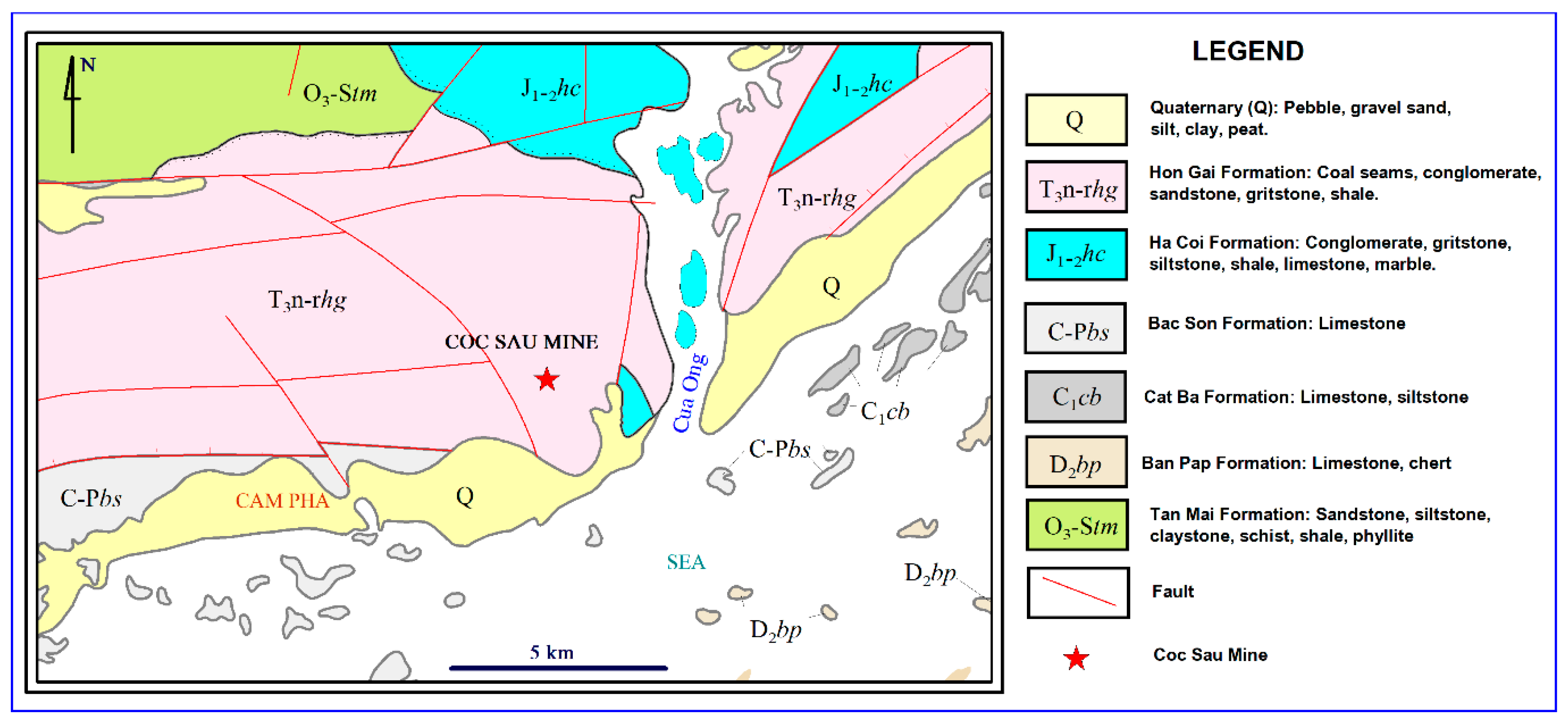
The Coc Sau open-cast coal mine was covered entirely by sedimentary rocks of the Late Triassic Hon Gai Formation (T3n-rhg) (Figure 2). The formation was composed of gritstone, conglomerate, sandstone, claystone, siltstone, shale, and coal seams. In general, these sedimentary rocks are quite hard with the Protodyakonov strength index (f) of 8 to 11 [62]. Therefore, fragmenting rocks by drilling-blasting was considered as an effective method for the exploitation of coal in the mine.
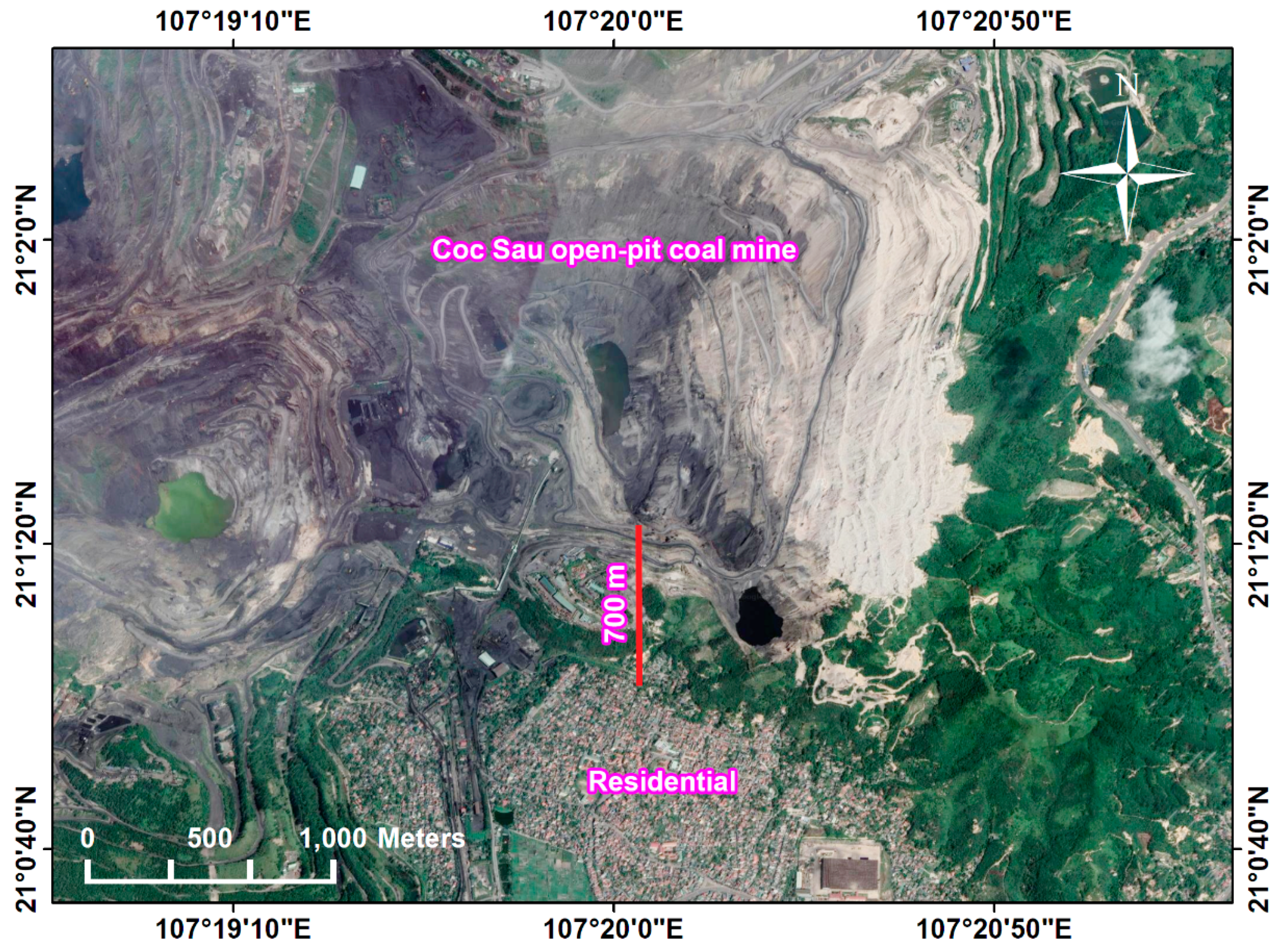
For drilling operations, CБIII-250, D245S, and DML were the favorite drills used in the mine. The borehole diameters used were in the range of 200 to 250 mm. For drilling, the average drilling speed was 10 to 15 m/h, so the amount of PM10 concentration incurred was not small. The drilling contributed to an increase in the impact of dust on the surrounding environment and public health. In this regard, the distance from the mine to the residential area is about 0.42 mile (~700 m); therefore, the effect of dust, especially the PM10 concentration, is significant (Figure 3). Also, the occupational hazard for employees is a particular concern.

3. Data Collection and Its Characteristics

As stated above, CБIII-250, D245S, and DML drills were used at the mine for drilling boreholes, with the diameter of boreholes in the range of 200 mm to 250 mm. For data collection, the drilling diameter/diameter of boreholes (d), the penetration rate of the drill (P), the moisture content (Wtn), the silt content (S), the density of rock mass (ρ), the compressive strength (σc), and the rebound hardness number (R) were used as independent variables to predict PM10 concentration.
As mentioned, CБIII-250, D245S, and DML were the component drills used in the mine with d in the range of 200 to 250 mm. With an average depth in the range of 12 to 15 m, the drills can penetrate the rock with P in the range of 0.16 to 0.41 m/min.
For humidity moisture (Wtn), the core drilling rock samples were carefully preserved and brought to the laboratory. Each drilling hole was collected as a sample by combining representative rock in the drilling core. In the laboratory, a total of 245 samples were used to determine the natural water content of rock (Wtn). The method was conducted by Vietnam’s standard of TCVN 10321:2014 [63]. The equation (1) for calculating the natural water content of the rock is as follows:
W t n = g 1 g 2 g 2 g 0 · 100
where g0, g1, g2 are the weights of the sample box without a rock sample, of the sample box and the natural rock sample, and of the sample box and the dried rock sample, respectively.
For silt content (S), the fine particles present in the drill cutting was determined (in %). For determining the properties of rock mass (ρ, σc), indirect experiments in combination with Protodiakonov’s strength index were used. To determine R, a rebound hardness tester was used, i.e., a Schmidt hammer.
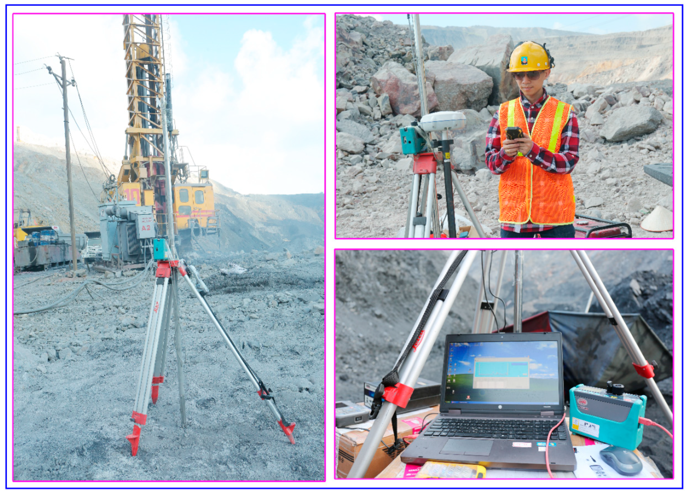
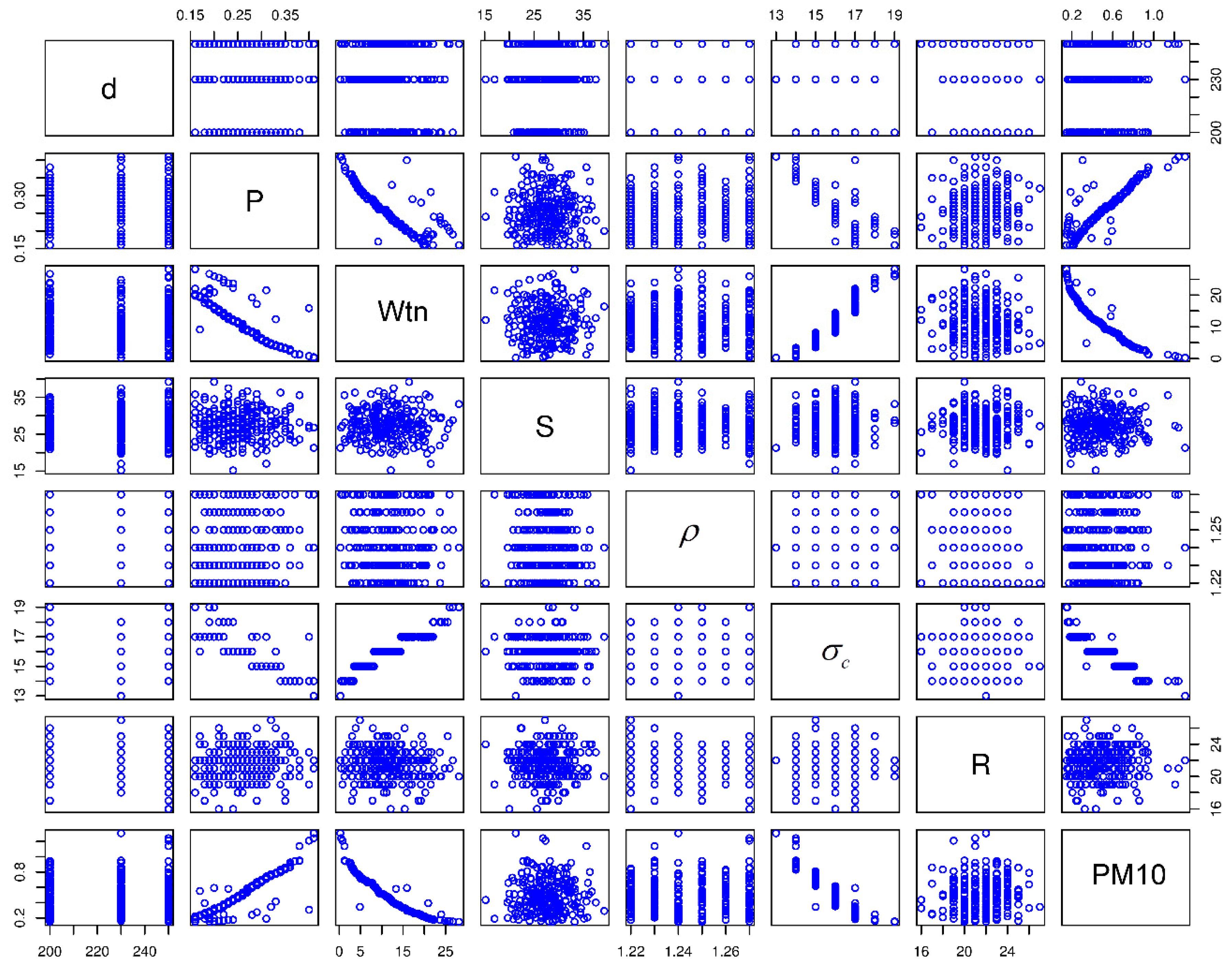
For measuring PM10 concentration, KANOMAX digital dust monitor model 3442 was used in this study (the manual of KANOMAX can be found at the following link https://kanomax.biz/asia/products/dust_monitors/model_3442_3443.html). This instrument (model 3442) is a light scattering portable dust monitor using a semiconductor laser radiation light source [64]. The principle of this method is that when the dust is irradiated, the scattered light intensity from the dust is proportional to the mass concentration. Two monitoring stations with this instrument were installed: One in the upstream and the other in the downstream. To ensure the accuracy of the predictive models, the datasets from independent drilling locations were collected to eliminate the maximum of PM10 concentration from other mining operations. In other words, there were no other activities (e.g., loading/unloading, transporting, blasting) on the same work sites of the drilling operation. Furthermore, the dust monitor was set around the drill with the distance being in the range of 5 to 10 m to ensure a maximum of PM10 concentration from the drilling operation was obtained (Figure 3). With 245 drilling operations, PM10 concentration was measured in the range of 0.148 to 1.306 gm/s. Figure 4 illustrates the data collection process for this study, and the data used is summarized in Table 2. Also, Figure 5 shows the relationship between input and output variables used in this study.
In Figure 5, the spread of the points denotes the relationship between the variables. Each sub-figure means the relationship between two variables. Note that the matrix is symmetrical. The correlated attributes showed good structure in their relationship, such as ρ, Wtn, and P. They are not linear, but good predictable curved relationships. Also, Figure 5 shows that the correlation of most of the input variables was not high. It is a right candidate for AI techniques in finding out the association between the input and output variables.

4. Compositions Analysis of PM10 from Drilling Operations

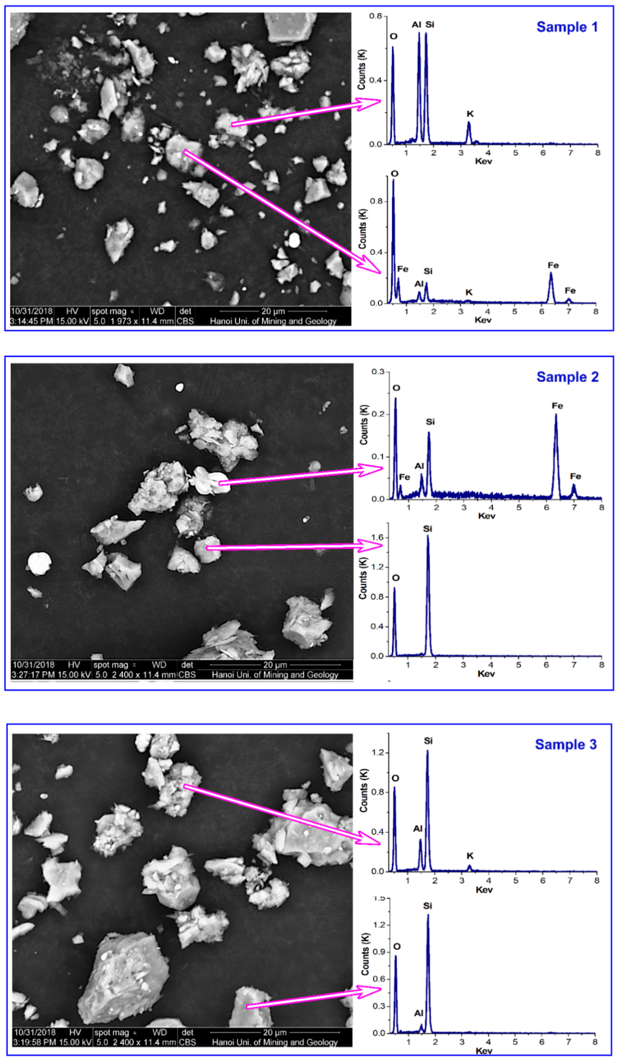
To assess the danger level of PM10 from drilling operations to community health and surroundings, the compositions of PM10 from drilling operations at the Coc Sau open-pit coal mine were analyzed by energy dispersive X-ray spectroscopy (SEM-EDS) (Quanta 450—FEI Company, Hillsboro, OR, USA). Accordingly, three dust samples of different boreholes were collected at the Coc Sau open-pit coal mine for analysis of their size and composition. The results from the scanning electron microscope coupled with SEM-EDS showed that the dust particles from the drilling process in the study area were relatively small with a size of less than ten μm. The composition of the dust consisted of many different elements, such as Al, Si, K, Fe (Figure 6), which are very dangerous for human health when breathed in. Therefore, accurate predictions of PM10 concentration from drilling operations in open-pit mines are necessary to minimize impact on public health and the surrounding environment.

5. The Principle of Intelligence Techniques

5.1. Random Forest (RF)

In this section, the RF is briefly presented. It is well-known as a decision tree algorithm, which was proposed by Breiman [65]. RF is a classification or regression technique using classification or regression trees in a group as a forest. Inspired by the development of the forest, each tree in the forest is treated as a decision. For regression problems (such as estimating PM10 concentration from drilling operations in this study), the average value of voters is selected as the final decision of the RF model as well. In other hands, RF is considered as an ensemble learning method based on the propensity of each tree [66]. It uses the bagging technique and decision tree algorithm like the CART algorithm to build an extensive collection of the correlate-decision trees. In statistics, RF uses the bagging technique as an ensemble tool to improve the accuracy and stability of models. The bootstrap technique with replacement is also used by RF to generate decision trees without prune [67]. For each bootstrap sample, a model is developed as a predictor. An ensemble of predictors and its average value is computed for the final decision of the RF (for regression problems) as follows (Equation (2)):
f ^ ( x ) = 1 N n = 1 N f ^ n ( x )
where N denotes the number of bootstrap samples; b denotes predictor; f ^ ( x ) denotes the prediction of the n model on an observation x.
A literature review showed that the RF algorithm has never been used to estimate PM10 concentration from drilling operations; for this study, it was considered and developed for estimating PM10 concentration from drilling operations. The background of the RF algorithm can be further found in [68,69,70,71].

5.2. Support Vector Regression (SVR)

SVR is one of the branches of the support vector machine (SVM) algorithm, one of the benchmark algorithms used in machine learning first introduced by Vapnik [72]. It has two main categories, including SVR and SVC (support vector classification). Of those, SVR is considered as the most common application form of continuous problems. The details of the SVR is presented in reference [73]. Also, kernel functions can be applied for regression problems (Equations (3)–(6)), including:
Linear function:
T ( a , b ) = a b
Polynomial function:
T ( a , b ) = [ ( a b ) + 1 ] d ; d ( 1 , n )
Radial original kernel function:
T ( a , b ) = exp [ a b 2 σ 2 ]
Two-layer neural function:
T ( a , b ) = tanh [ e ( a b ) δ ]
Like the RF algorithm, a review of previous works showed that the SVR algorithm has never been used to estimate PM10 concentration from drilling operations. Therefore, it was considered and combined with the PSO algorithm for estimating PM10 concentration from drilling operations in this study. More principles of the SVR algorithm can be seen in [72,73,74,75,76,77].

5.3. Classification and Regression Tree (CART)

CART is a statistical technique proposed by Breiman [78]. It can solve both regression and classification problems for exploring as well as modeling data. CART was also developed based on decision trees to explain the variation of the dependent variable by one or more independent variables [79]. As a “white box” algorithm, the relationship between dependent and independent variables is more straightforward with the CART algorithm [80,81]. It does not consider any previous assumptions related to the relationship between variables. Instead, the repeatedly split data process is applied to construct the tree based on an independent variable. The data is separated into two reciprocally exclusive clusters at each split, each of which is as much the same as possible. Then, the separation process is held to each group independently. Yes/no answers concerning the predictor values are the primary basis for generating a binary tree by the CART algorithm.
For developing a CART model for predicting PM10 concentration, the four main steps of the CART algorithm are conducted as below:
  • Applying some rules to exploit data at a node based on a variable value;
  • Using some criteria to prevent the creation of complex trees;
  • Pruning for optimum performance of the model;
  • Calculation and prediction of the output for terminal nodes.
As with the RF and SVR algorithms, a review of previous studies show that the CART algorithm has never been used to estimate PM10 concentration from drilling operations. Therefore, it is considered and developed in this study. More background of the CART algorithm can be referred to at [82,83,84,85,86].

5.4. K-Nearest Neighbors (KNN)

KNN is one of the “learning lazy” algorithms, which can be used/applied for regression as well as classification problems [87]. KNN aims to find the number of nearest neighbors (k) from a functional space. To obtain this goal, the Euclidean distance x y between the input variables and queries is calculated as Equation (7). Then, the k closest input points for the consultation is determined.
d ( a t , a i ) = n = 1 N W n ( a t , n a i , n ) 2
where N is the features number; αi,n is the nth feature value of the training point αi; αt,n; is the nth feature value of the testing point αt; Wn is the weight of the nth feature, 0 W n 1 .
For estimating a regression problem (such as predicting PM10 concentration in this study), a kernel function is often applied to calculate Wn based on its proximity to the testing point (Equation (8)), as follows:
f ^ ( a t ) = i = 1 k ϕ ( a t , a ( i ) ) f ( a ( i ) ) i = 1 k ϕ ( a t , a ( i ) )
Where ϕ ( a t , a ( i ) ) denotes a kernel function at the ith training point αi; f ( a ( i ) ) indicates the response of αi.
Like the RF, SVR, and CART algorithms, a review of the literature showed that the KNN algorithm has never been used to estimate PM10 concentration from drilling operations, and is considered and developed to predict PM10 concentration from drilling operations in this study. More principles of KNN algorithm can be seen in [42,87,88,89].

5.5. Particle Swarm Optimization (PSO) Algorithm

PSO is a swarm algorithm inspired by the behavior of the particles/social animals, such as fish or birds. It was introduced and developed by Eberhart and Kennedy [90] and classified as one of the metaheuristic techniques. It was considered as an evolutionary computation technique in the statistical community [41]. The PSO algorithm implements six steps for optimal searching as the following procedure. In which, the velocity and local positions are continuously updated using Equations (9) and (10), for sharing their experience.
  • Generate the particle swarm size with random locations and speeds on d dimensions in the subject space.
  • Estimate the proper optimization fitness function for each particle in d factors.
  • Compare the fitness evaluation with pbest of the particle. If the present value is better than pbest, then set pbest value equal to the present value, and the pbest position equal to the current position in d-dimensional space.
  • Compare the evaluation of the fitness with the overall previous best of the population. If the current value is better than gbest, then reset gbest to the current population index and value of particle.
  • Change the velocity and local of the particle as Equations (9) and (10) as follow:
    v j i + 1 = w v j ( i ) + ( c 1 × r 1 × ( l o c a l   b e s t j x j ( i ) ) ) + ( c 2 × r 2 × ( global   b e s t j x j ( i ) ) ) , v min v j ( i ) v max
    x j i + 1 = x j ( i ) + v j ( i + 1 ) ; j = 1 , 2 , , n
    where x j ( i ) denote the position of particle j at iteration i; v j ( i ) denote the velocity of particle j at iteration i; w is the inertial weight coefficient; i is the iteration number; r1 and r2 represent a random number uniformly distributed in [0,1] which is randomly generated at iteration and for each particle.
  • Loop to step (2) until a criterion is met. Usually, the maximum number of iterations or sufficiently good fitness, the searching process will stop.
In this study, the PSO algorithm was used/applied to optimize the hyper-parameters of the SVR model with different kernel functions (i.e., radial basis function, polynomial, linear) for predicting PM10 concentration from drilling operations.

5.6. Development of the PM10 Concentration Predictive Models

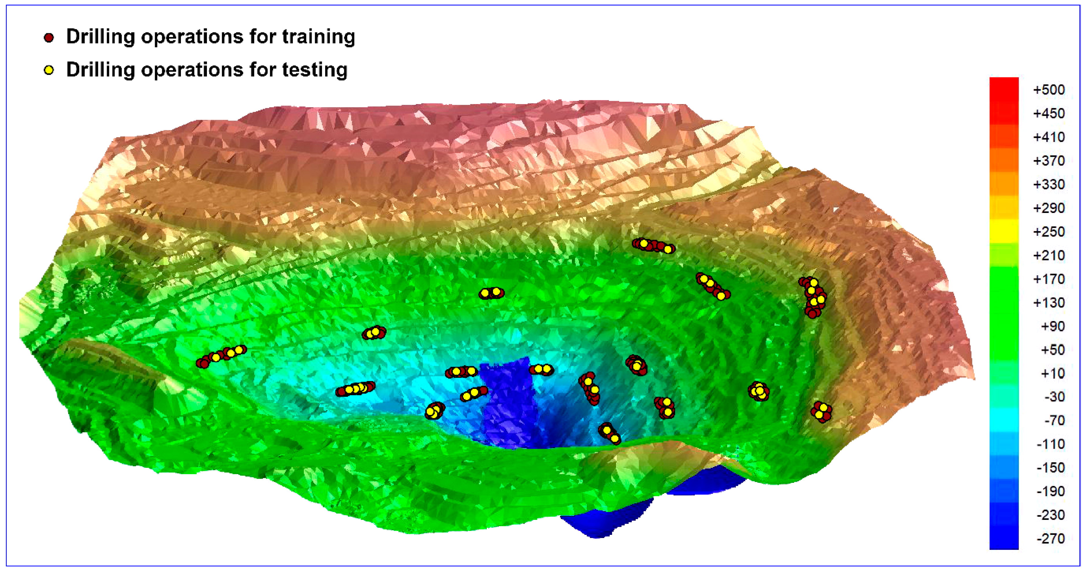
To establish the PM10 concentration predictive models, a database including 245 drilling operations was randomly divided into two phases. In the first phase, ~80% of the data (approximately 221 observations) was used for the development of the models. The remaining ~20% (around 24 observations) in the second phase was used as new data for validating the performance of the developed models. ArcGIS software was used to manage databases with big data query capabilities [91]. The preparation of data for this study is illustrated in Figure 7.
To validate/evaluate the models performances, two performance indicators, the root-mean-squared error (RMSE) and the determination coefficient (R2), were calculated (Equations (11) and (12)):
RMSE = 1 n i = 1 n ( y i y i ^ ) 2
R 2 = 1 i ( y i y ^ i ) 2 i ( y i y ¯ ) 2
where n is a total number of data; y i , y ^ i and y ¯ are measured, predicted, and mean of y i values, respectively. For an optimal model, R2 = 1 and RMSE = 0.

5.7. RF Model

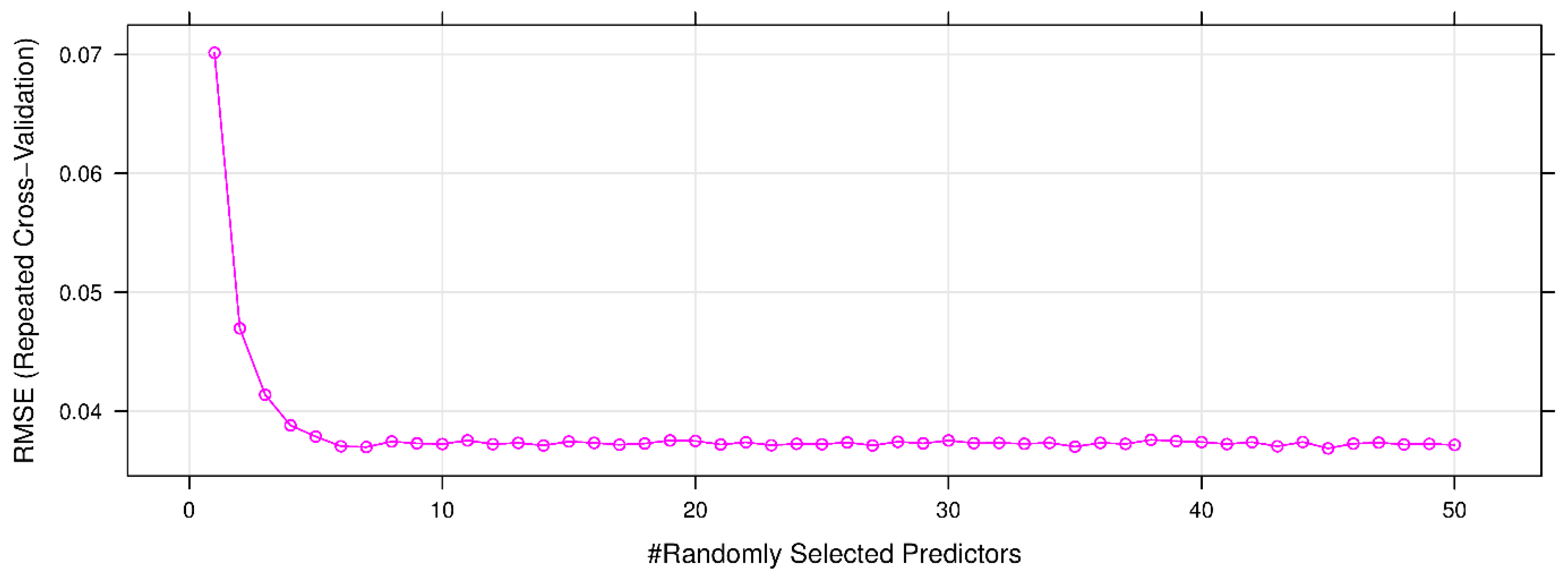
For the RF model, the number of decision trees (ntree) and the random predictor selected (mtry) are considered as the essential criteria for measuring the quality of the model. To ensure the diversity of the forest, ntree was selected equal to 2000 [71] in this study. Each decision tree plays a role as a voter in the RF model. The remaining parameter, i.e., mtry was selected by a grid search technique with mtry in the range of 1 to 50 (Figure 8). Also, k-fold cross-validation resampling technique was applied with k = 10 to avoid overfitting/underfitting. As a result, the optimal values of the RF model for anticipating PM10 concentration was obtained at ntree = 2000 and mtry = 45.

5.8. CART Model

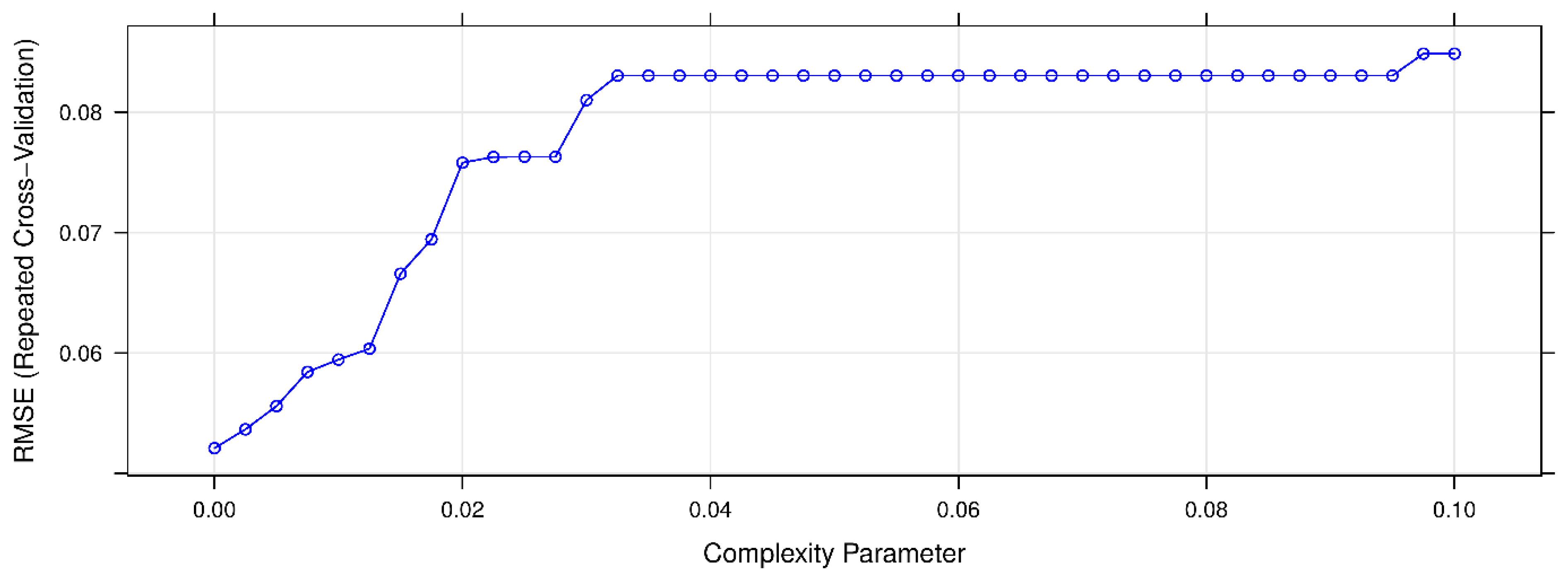
For the CART model, the complexity parameter (cp) was used to tune the performance of the model. Similar to the RF model, a grid search with the cp in the range of 0 to 0.1 was conducted. The 10-fold cross-validation resampling technique was also used to avoid overfitting/underfitting, as those used for the RF model. Eventually, the CART model obtained the best performance at cp = 0 for estimating PM10 concentration, as shown in Figure 9.

5.9. KNN Model

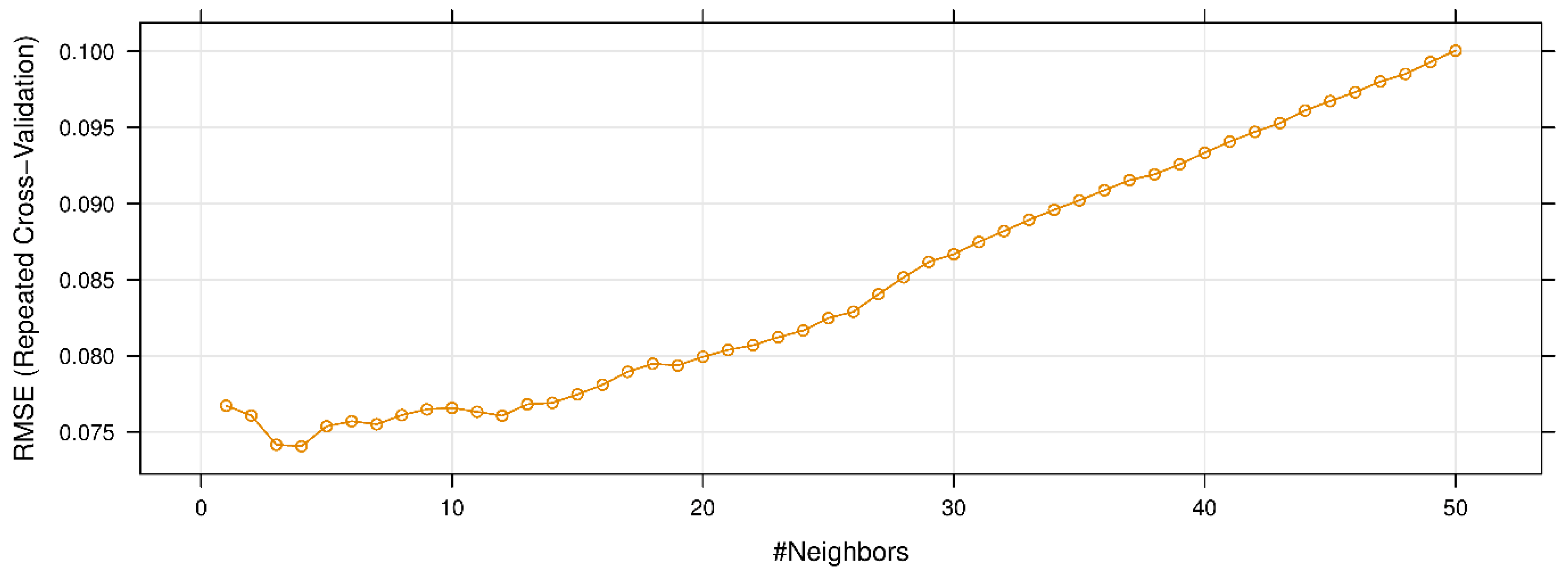
For the KNN model, its performance is controlled by the number of neighbors (k). Similar to the RF and CART models, a grid search with the k in the range of 1 to 50 was conducted to find out the best KNN model. The 10-fold cross-validation technique with three repeats was also used to avoid overfitting/underfitting of the KNN model. Finally, a good KNN model was found at k = 4, as shown in Figure 10.

5.10. PSO-SVR Models for Estimating PM10 Concentration

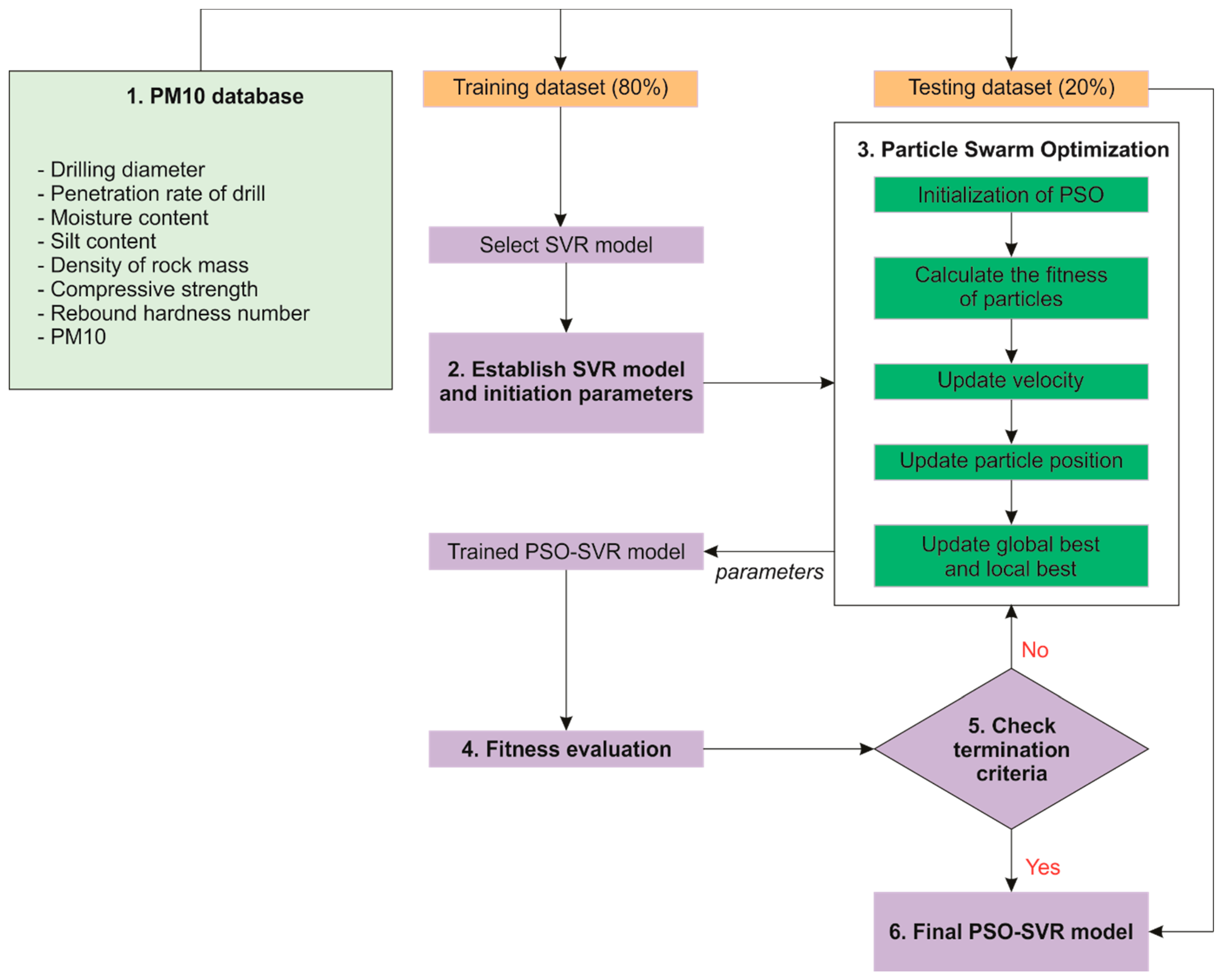
As introduced above, the primary purpose of this study is developing and proposing a new artificial intelligence system for predicting PM10 concentration, i.e., PSO-SVR model. Three forms of kernel function were applied for the development of the PSO-SVR models, abbreviated as PSO-SVR-L, PSO-SVR-P, and PSO-SVR-RBF models. In this procedure, the PSO algorithm performs a global search for the optimal values of SVR models through a fitness function, i.e., RMSE (Equation 11). For each PSO-SVR model, the hyper-parameters are different. Depending on the kernel function used, the hyper-parameters of each PSO-SVR model are different. Table 3 shows the hyper-parameters of the PSO-SVR models with different functions of the kernel. A framework of the PSO-SVR model for estimating concentration in this study is shown in Figure 11.
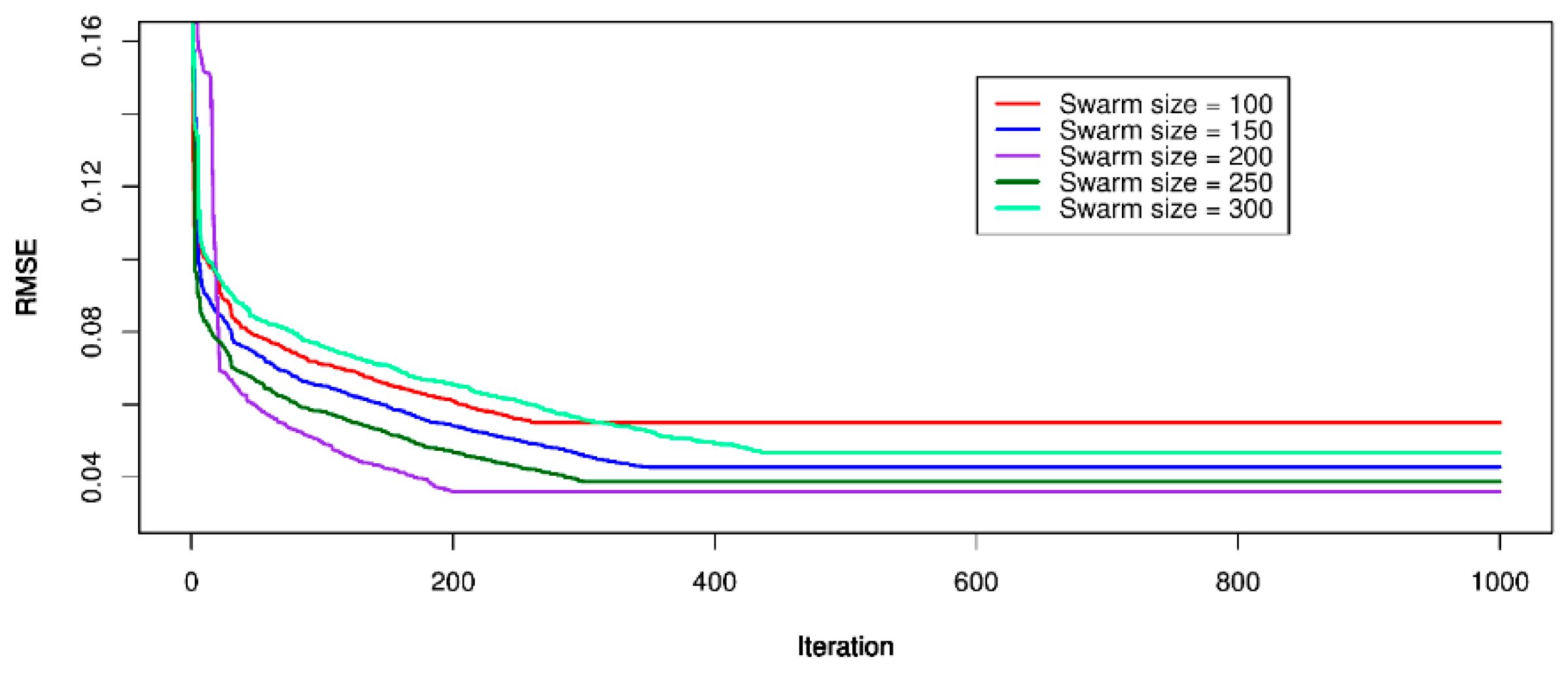
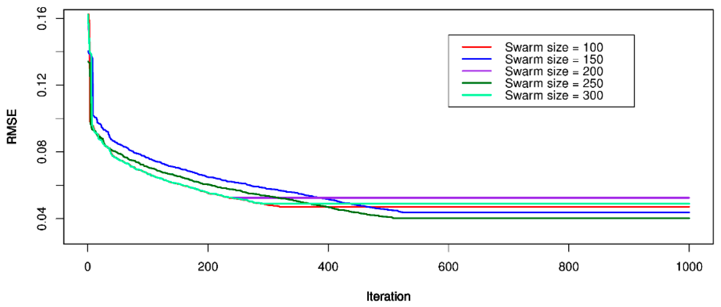
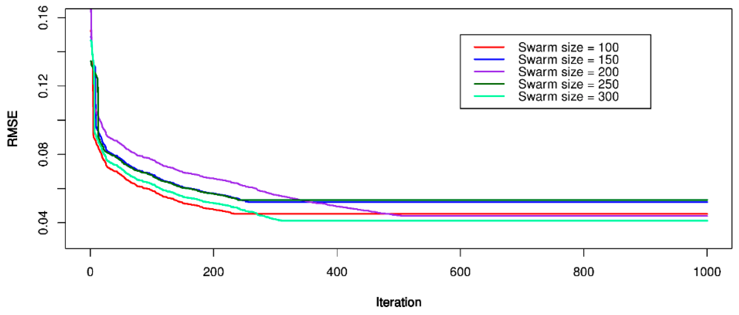
Before proceeding to search for the optimal values of hyper-parameters of the SVR models, the parameters of the PSO algorithm is set as the first step on the training dataset. In the PSO algorithm, the number population (p), maximum number of iteration (mi), maximum particle’s velocity (Vmax), individual cognitive ( ϕ 1 ), group cognitive ( ϕ 2 ), and inertia weight (w) are the parameters used for the optimization process. The sample size should have functional population diversity [92,93,94], therefore, a trial-and-error procedure was employed with the swarm size was 100, 150, 200, 250, 300, respectively (p = 50, 100, 150, 200, 250, 300). For terminating the optimization process in this study, mi was set equal to 1000 to check the fitness of particle positions using the RMSE metric (Equation 11). To ensure the balance between global discovery and local search, w was set equal to 0.9 [95]. According to Kennedy [96] and Clerc and Kennedy [97], ϕ 1 should be equal to ϕ 2 and ϕ 1 + ϕ 2 lie in the range of 0 to 4. Therefore, in this study, ϕ 1 = ϕ 2 = 1.6. To ensure convergence and prevent explosion [98], Vmax was set equal to 2 in this study. Figure 12, Figure 13 and Figure 14 shows the training process of PSO-SVR models (PSO-SVR-L; PSO-SVR-P; PSO-SVR-RBF).
After the optimization process of the PSO algorithm was stopped, the optimal values of the SVR models were extracted for predicting PM10 concentration. Table 4 shows the obtained results by the PSO algorithm for searching the hyper-parameters of the SVR models.

6. Results and Discussion

Once the PM10 concentration predictive models were developed, their performance was evaluated and discussed through RMSE and R2, as mentioned in Equations (11) and (12). Table 5 shows the performance of the developed models on the training and testing datasets.
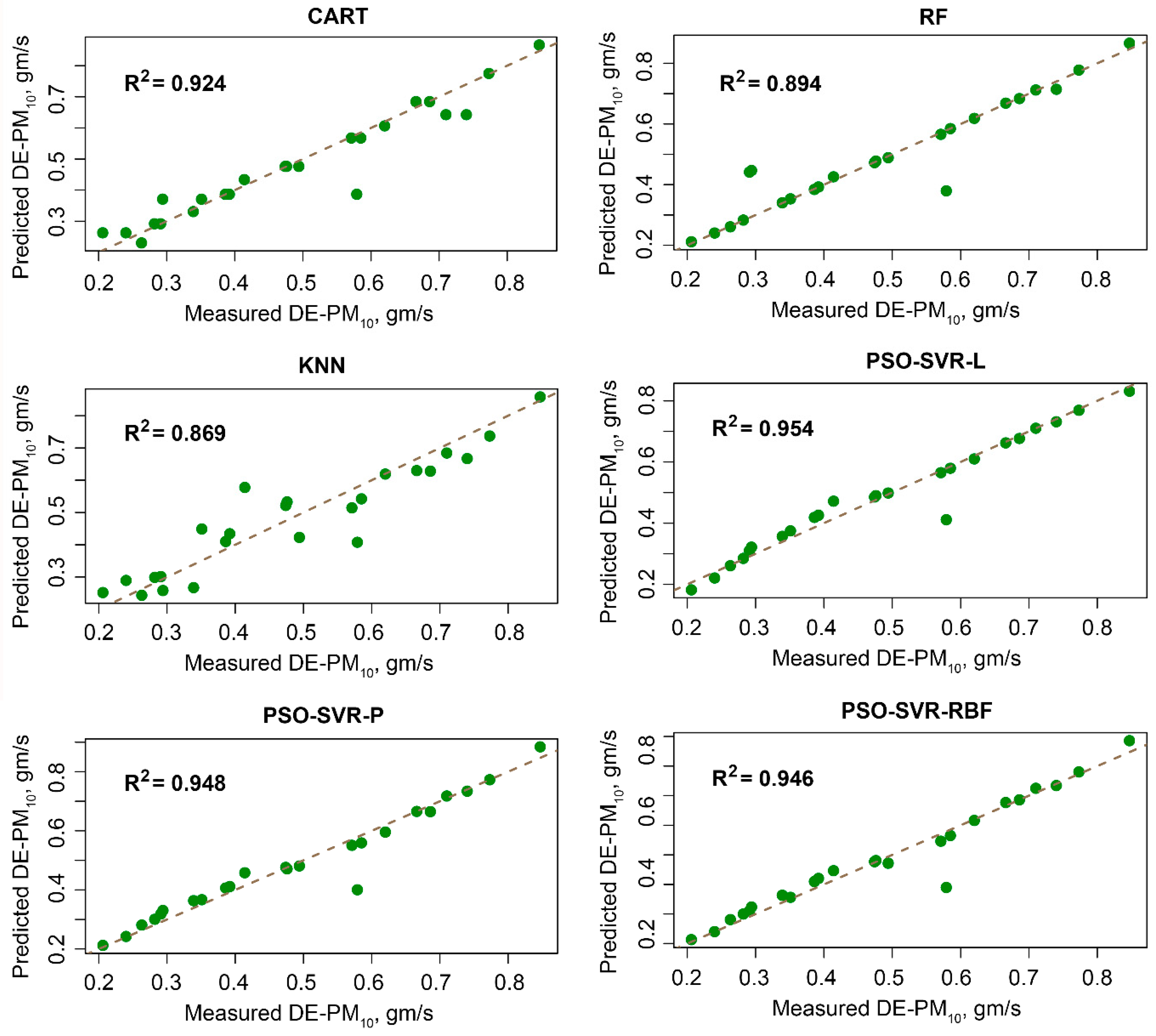
Table 5 showed that the PSO-SVR models performed very well in estimating PM10 concentration from drilling operations in this study with an RMSE in the range of 0.036 to 0.041 on the training dataset, 0.040 to 0.043 on the testing dataset; R2 in the range of 0.962 to 0.963 on the training dataset, 0.946 to 0.954 on the testing dataset. Notable, the PSO-SVR-L model yielded the best performance with an RMSE of 0.036 and 0.040 for the training and testing dataset, respectively; and R2 of 0.963 and 0.954 for the training and testing dataset, respectively. With the highest performance, the PSO-SVR-L model is the most dominant model for estimating PM10 concentration in this study. The remaining AI models (RF, CART, KNN) provided more mediocre performance than those of the PSO-SVR models with an RMSE in the range of 0.057 to 0.074 on the training dataset, 0.052 to 0.067 on the testing dataset; and R2 in the range of 0.904 to 0.963 on the training dataset, 0.867 to 0.924 on the testing dataset. Remarkable, the KNN model yielded the most inferior performance with an RMSE of 0.074 and 0.067 for the training and testing dataset, respectively; and R2 of 0.904 and 0.867 for the training and testing dataset, respectively. Figure 15 shows the measured versus predicted values of PM10 concentration on the testing dataset.
Based on the obtained results from the developed models, it can be seen that machine learning algorithms perform very well in estimating PM10 concentration from drilling operations in open-pit mines. In particular, the PSO algorithm played a significant role in optimizing the hyper-parameters of the SVR models to provide more accurate predictive results. The PSO-SVR-L model was introduced as the most superior model in this study for estimating PM10 concentration that explained the linear relationship of the input variables with PM10 concentration. However, the present study used seven independent/input variables for predicting PM10, and the effectiveness of the models was different. Therefore, an importance analysis procedure of the independent/input variables for each model was performed in this study, i.e., using the Hilbert-Schmidt Independence Criterion (HSIC) [99,100]. An overall picture of performance as well as the ability to explain the relationship between the independent/input variables of the models is illustrated in Table 6.
From Table 6, it is easy to recognize that P, Wtn, and σc are the most importance parameters of all developed AI models. They should be used for estimating PM10 concentration from drilling operations. Taking a closer look at Table 6 shows that the assessment of the importance of input variables has a significant effect on the performance of the model. In the proposed PSO-SVR-L model, the Wtn parameter was most importance parameter with indices of 0.975, whereas the remaining models were only evaluated in the range of 0.896 to 0.957. Likewise, P and σc also received different values from different models. It can be seen that the evaluation of the importance of input variables as too low or too high has a significant impact on the performance of the forecasting model.

7. Conclusions and Recommendations

Drilling-blasting is an essential task in mining operations. Until now, it is still the most efficient method for fragmenting rocks in open-cast mines. However, the impact on the environment caused by drilling operations as well as blasting operations is inevitable, especially in dust concentration. Evidence of the dangers of PM10 has been found in open-pit mines. Therefore, the prediction and strict control of PM10 concentrations is necessary to minimize the harmful impact on the surrounding environment. In this study, PM10 concentration from drilling operations in open-pit mines was considered and evaluated. In this study, some conclusions and remarks were drawn:
  • The dust concentration caused by activities in open-pit mines is high and very dangerous. The dust is the cause of the harmful impact on the environment and public health. In this study, PM10 concentration from drilling operations in open-pit mines was considered and predicted. However, the dust concentration caused by other activities in open-pit mines also needs to be controlled and predicted in the future. Total dust concentration needs to be managed in open-pit mines, and is a challenge for future works.
  • For drilling operations, AI techniques are the advanced methods for predicting drill-induced dust concentration. They provided predictive intelligence models with high accuracy in practical engineering. In addition to the ANN, which was developed by previous researchers, the other machine learning techniques, i.e., RF, CART, KNN, PSO-SVR in this study were also techniques to control air quality in open-pit mines.
  • The PSO algorithm is a robust tool for the optimization of the SVR model for estimating PM10 concentration. With an RMSE of 0.040 and R2 of 0.954, the proposed PSO-SVR-L model was the most dominant model for predicting drill-induced PM10 concentration in this study. It should be applied in practical engineering to control PM10 concentration from drilling operations as well as the other processes. Additionally, the CART, RF, and KNN models should also be considered in other conditions of different sites for predicting dust concentration. They can be good models in other case studies for predicting the environmental issues in open-pit mines.
  • ρ , W t n , and P are the most influential parameters on the PM10 concentration predictive model, especially W t n . They should be of particular interest and carefully collected for predicting drill-induced PM10 concentration.
  • Based on the obtained results of this study, PM10 concentration from drilling operations can be predicted and controlled by the proposed PSO-SVR model. However, there are several operations, such as blasting, transporting, loading/unloading, which are also the causes of dust generation in open-pit mines. Therefore, the feasibility of AI techniques is also needed to investigate and establish a comprehensive air quality control system in open-pit mines.

Author Contributions

Data collection and experimental works: H.-B.B., N.Q.L., Q.-T.L., V.-D.N., N.-B.N.; Writing, discussion, analysis: X.-N.B., C.W.L., H.N., H.M.

Funding

This research received no external funding.

Acknowledgments

This work was financially supported by the Ministry of Education and Training (MOET) in Viet Nam under grant number B2018-MDA-03SP. The authors also thank the Center for Mining, Electro-Mechanical Research of Hanoi University of Mining and Geology (HUMG), Vietnam; the engineers and leaders of the Coc Sau open-pit coal mine, Quang Ninh province, Vietnam for their help and cooperation.

Conflicts of Interest

The authors declare no conflict of interest.

References

  1. Albert, S.; Kvennefors, C.; Jacob, K.; Kera, J.; Grinham, A. Environmental change in a modified catchment downstream of a gold mine, Solomon Islands. Environ. Pollut. 2017, 231, 942–953. [Google Scholar] [CrossRef] [PubMed]
  2. Bascetin, A. A decision support system using analytical hierarchy process (AHP) for the optimal environmental reclamation of an open-pit mine. Environ. Geol. 2007, 52, 663–672. [Google Scholar] [CrossRef]
  3. Huertas, J.I.; Huertas, M.E.; Izquierdo, S.; González, E.D. Air quality impact assessment of multiple open pit coal mines in northern Colombia. J. Environ. Manag. 2012, 93, 121–129. [Google Scholar] [CrossRef] [PubMed]
  4. Alvarenga, P.; Palma, P.; De Varennes, A.; Cunha-Queda, A.C. A contribution towards the risk assessment of soils from the São Domingos Mine (Portugal): Chemical, microbial and ecotoxicological indicators. Environ. Pollut. 2012, 161, 50–56. [Google Scholar] [CrossRef] [PubMed]
  5. Chakraborty, M.; Ahmad, M.; Singh, R.; Pal, D.; Bandopadhyay, C.; Chaulya, S. Determination of the emission rate from various opencast mining operations. Environ. Model. Softw. 2002, 17, 467–480. [Google Scholar] [CrossRef]
  6. Li, J.; Chen, B.; de la Campa, A.M.S.; Alastuey, A.; Querol, X.; Jesus, D. 2005–2014 trends of PM10 source contributions in an industrialized area of southern Spain. Environ. Pollut. 2018, 236, 570–579. [Google Scholar] [CrossRef] [PubMed]
  7. Vicente, A.; Juan, P.; Meseguer, S.; Díaz-Avalos, C.; Serra, L. Variability of PM10 in industrialized-urban areas. New coefficients to establish significant differences between sampling points. Environ. Pollut. 2018, 234, 969–978. [Google Scholar] [CrossRef] [PubMed]
  8. Gautam, S.; Patra, A.K.; Prusty, B.K. Opencast mines: A subject to major concern for human health. Int. Res. J. Geol. Min. 2012, 2, 25–31. [Google Scholar]
  9. Wheeler, A.; Williams, I.; Beaumont, R.; Hamilton, R. Characterisation of particulate matter sampled during a study of children’s personal exposure to airborne particulate matter in a UK urban environment. Environ. Monit. Assess. 2000, 65, 69–77. [Google Scholar] [CrossRef]
  10. Reed, W. Significant Dust Dispersion Models for Mining Operations; National Institute for Accupational Safety and Health: Atlanta, GA, USA, 2005.
  11. Espitia-Perez, L.; da Silva, J.; Espitia-Perez, P.; Brango, H.; Salcedo-Arteaga, S.; Hoyos-Giraldo, L.S.; de Souza, C.T.; Dias, J.F.; Agudelo-Castaneda, D.; Toscano, A.V. Cytogenetic instability in populations with residential proximity to open-pit coal mine in Northern Colombia in relation to PM10 and PM2.5 levels. Ecotoxicol. Environ. Saf. 2018, 148, 453–466. [Google Scholar] [CrossRef]
  12. Chaulya, S. Air quality status of an open pit mining area in India. Environ. Monit. Assess. 2005, 105, 369–389. [Google Scholar] [CrossRef] [PubMed]
  13. Pokorná, P.; Hovorka, J.; Brejcha, J. Impact of Mining Activities on the Air Quality in The Village Nearby a Coal Strip Mine. In IOP Conference Series: Earth and Environmental Science; IOP Publishing: Bristol, England, 2016. [Google Scholar]
  14. Alvarado, M.; Gonzalez, F.; Erskine, P.; Cliff, D.; Heuff, D. A methodology to monitor airborne PM10 dust particles using a small unmanned aerial vehicle. Sensors 2017, 17, 343. [Google Scholar] [CrossRef] [PubMed]
  15. Armaghani, D.J.; Hajihassani, M.; Marto, A.; Faradonbeh, R.S.; Mohamad, E.T. Prediction of blast-induced air overpressure: A hybrid AI-based predictive model. Environ. Monit. Assess. 2015, 187, 666. [Google Scholar] [CrossRef] [PubMed]
  16. Armaghani, D.J.; Hajihassani, M.; Mohamad, E.T.; Marto, A.; Noorani, S. Blasting-induced flyrock and ground vibration prediction through an expert artificial neural network based on particle swarm optimization. Arab. J. Geosci. 2014, 7, 5383–5396. [Google Scholar] [CrossRef]
  17. Ghose, M.K.; Majee, S. Sources of air pollution due to coal mining and their impacts in Jharia coalfield. Environ. Int. 2000, 26, 81–85. [Google Scholar] [CrossRef]
  18. Chaulya, S. Assessment and management of air quality for an opencast coal mining area. J. Environ. Manag. 2004, 70, 1–14. [Google Scholar] [CrossRef]
  19. Dastoor, A.P.; Pudykiewicz, J. A numerical global meteorological sulfur transport model and its application to Arctic air pollution. Atmos. Environ. 1996, 30, 1501–1522. [Google Scholar] [CrossRef]
  20. Binkowski, F.; Ching, J. Modeling Fine Particulate Mass and Visibility Using the EPA Regional Particulate Model; American Meteorological Society: Boston, MA, USA, 1996. [Google Scholar]
  21. Saltbones, J.; Foss, A.; Bartnicki, J. Norwegian Meteorological Institute’s real-time dispersion model SNAP (Severe Nuclear Accident Program): Runs for ETEX and ATMES II experiments with different meteorological input. Atmos. Environ. 1998, 32, 4277–4283. [Google Scholar] [CrossRef]
  22. Cohn, R.D.; Eder, B.K.; Leduc, S.K.; Dennis, R.L. Development of an aggregation and episode selection scheme to support the Models-3 Community Multiscale Air Quality Model. J. Appl. Meteorol. 2001, 40, 210–228. [Google Scholar] [CrossRef]
  23. Vardoulakis, S.; Fisher, B.E.; Pericleous, K.; Gonzalez-Flesca, N. Modelling air quality in street canyons: A review. Atmos. Environ. 2003, 37, 155–182. [Google Scholar] [CrossRef]
  24. Nagesha, K.; Singh, M.; Chandra, G.R. Development of empirical model to predict particulate matter. AIP Conf. Proc. 2018, 1992, 040013. [Google Scholar]
  25. Aneja, V.P.; Isherwood, A.; Morgan, P. Characterization of particulate matter (PM10) related to surface coal mining operations in Appalachia. Atmos. Environ. 2012, 54, 496–501. [Google Scholar] [CrossRef]
  26. Nguyen, H.; Bui, X.-N.; Bui, H.-B.; Mai, N.-L. A comparative study of artificial neural networks in predicting blast-induced air-blast overpressure at Deo Nai open-pit coal mine, Vietnam. Neural Comput. Appl. 2018. [Google Scholar] [CrossRef]
  27. Ghose, M.K. Generation and quantification of hazardous dusts from coal mining in the Indian context. Environ. Monit. Assess. 2007, 130, 35–45. [Google Scholar] [CrossRef] [PubMed]
  28. Asteris, P.; Kolovos, K.; Douvika, M.; Roinos, K. Prediction of self-compacting concrete strength using artificial neural networks. Eur. J. Environ. Civ. Eng. 2016, 20, s102–s122. [Google Scholar] [CrossRef]
  29. Asteris, P.; Roussis, P.; Douvika, M. Feed-forward neural network prediction of the mechanical properties of sandcrete materials. Sensors 2017, 17, 1344. [Google Scholar] [CrossRef] [PubMed]
  30. Asteris, P.G.; Nikoo, M. Artificial bee colony-based neural network for the prediction of the fundamental period of infilled frame structures. Neural Comput. Appl. 2019. [Google Scholar] [CrossRef]
  31. Asteris, P.G.; Nozhati, S.; Nikoo, M.; Cavaleri, L.; Nikoo, M. Krill herd algorithm-based neural network in structural seismic reliability evaluation. Mech. Adv. Mater. Struct. 2019, 26, 1–8. [Google Scholar] [CrossRef]
  32. Asteris, P.G.; Plevris, V. Anisotropic masonry failure criterion using artificial neural networks. Neural Comput. Appl. 2017, 28, 2207–2229. [Google Scholar] [CrossRef]
  33. Asteris, P.G.; Tsaris, A.K.; Cavaleri, L.; Repapis, C.C.; Papalou, A.; Di Trapani, F.; Karypidis, D.F. Prediction of the fundamental period of infilled RC frame structures using artificial neural networks. Comput. Intell. Neurosci. 2016, 2016, 20. [Google Scholar] [CrossRef]
  34. Cavaleri, L.; Chatzarakis, G.E.; Trapani, F.D.; Douvika, M.G.; Roinos, K.; Vaxevanidis, N.M.; Asteris, P.G. Modeling of surface roughness in electro-discharge machining using artificial neural networks. Adv. Mater. Res. 2017, 6, 169–184. [Google Scholar]
  35. Chen, H.; Asteris, P.G.; Jahed Armaghani, D.; Gordan, B.; Pham, B.T. Assessing Dynamic Conditions of the Retaining Wall: Developing Two Hybrid Intelligent Models. Appl. Sci. 2019, 9, 1042. [Google Scholar] [CrossRef]
  36. Plevris, V.; Asteris, P.G. Modeling of masonry failure surface under biaxial compressive stress using Neural Networks. Constr. Build. Mater. 2014, 55, 447–461. [Google Scholar] [CrossRef]
  37. Le, L.T.; Nguyen, H.; Dou, J.; Zhou, J. A Comparative Study of PSO-ANN, GA-ANN, ICA-ANN, and ABC-ANN in Estimating the Heating Load of Buildings’ Energy Efficiency for Smart City Planning. Appl. Sci. 2019, 9, 2630. [Google Scholar] [CrossRef]
  38. Bui, X.-N.; Muazu, M.A.; Nguyen, H. Optimizing Levenberg–Marquardt backpropagation technique in predicting factor of safety of slopes after two-dimensional OptumG2 analysis. Eng. Comput. 2019. [Google Scholar] [CrossRef]
  39. Zhang, X.; Nguyen, H.; Bui, X.-N.; Tran, Q.-H.; Nguyen, D.-A.; Bui, D.T.; Moayedi, H. Novel Soft Computing Model for Predicting Blast-Induced Ground Vibration in Open-Pit Mines Based on Particle Swarm Optimization and XGBoost. Nat. Resour. Res. 2019. [Google Scholar] [CrossRef]
  40. Shang, Y.; Nguyen, H.; Bui, X.-N.; Tran, Q.-H.; Moayedi, H. A Novel Artificial Intelligence Approach to Predict Blast-Induced Ground Vibration in Open-pit Mines Based on the Firefly Algorithm and Artificial Neural Network. Nat. Resour. Res. 2019. [Google Scholar] [CrossRef]
  41. Nguyen, H.; Moayedi, H.; Foong, L.K.; Al Najjar, H.A.H.; Jusoh, W.A.W.; Rashid, A.S.A.; Jamali, J. Optimizing ANN models with PSO for predicting short building seismic response. Eng. Comput. 2019. [Google Scholar] [CrossRef]
  42. Nguyen, H.; Bui, X.-N.; Tran, Q.-H.; Mai, N.-L. A new soft computing model for estimating and controlling blast-produced ground vibration based on hierarchical K-means clustering and cubist algorithms. Appl. Soft Comput. 2019, 77, 376–386. [Google Scholar] [CrossRef]
  43. Armaghani, D.J.; Hajihassani, M.; Monjezi, M.; Mohamad, E.T.; Marto, A.; Moghaddam, M.R. Application of two intelligent systems in predicting environmental impacts of quarry blasting. Arab. J. Geosci. 2015, 8, 9647–9665. [Google Scholar] [CrossRef]
  44. Armaghani, D.J.; Hajihassani, M.; Sohaei, H.; Mohamad, E.T.; Marto, A.; Motaghedi, H.; Moghaddam, M.R. Neuro-fuzzy technique to predict air-overpressure induced by blasting. Arab. J. Geosci. 2015, 8, 10937–10950. [Google Scholar] [CrossRef]
  45. Chelani, A.B.; Gajghate, D.; Hasan, M. Prediction of ambient PM10 and toxic metals using artificial neural networks. J. Air Waste Manag. Assoc. 2002, 52, 805–810. [Google Scholar] [CrossRef] [PubMed]
  46. McKendry, I.G. Evaluation of artificial neural networks for fine particulate pollution (PM10 and PM2.5) forecasting. J. Air Waste Manag. Assoc. 2002, 52, 1096–1101. [Google Scholar] [CrossRef] [PubMed]
  47. Lal, B.; Tripathy, S.S. Prediction of dust concentration in open cast coal mine using artificial neural network. Atmos. Pollut. Res. 2012, 3, 211–218. [Google Scholar] [CrossRef] [Green Version]
  48. Alkasassbeh, M.; Sheta, A.F.; Faris, H.; Turabieh, H. Prediction of PM10 and TSP air pollution parameters using artificial neural network autoregressive, external input models: A case study in salt, Jordan. Middle-East J. Sci. Res. 2013, 14, 999–1009. [Google Scholar]
  49. Mishra, D.; Goyal, P.; Upadhyay, A. Artificial intelligence based approach to forecast PM2.5 during haze episodes: A case study of Delhi, India. Atmos. Environ. 2015, 102, 239–248. [Google Scholar] [CrossRef]
  50. Nagesha, K.; Chandar, K.R.; Sastry, V. Prediction of Dust Dispersion by Drilling Operation Using Artificial Neural Networks. Int. J. Prev. Control Ind. Pollut. 2016, 1, 1–13. [Google Scholar]
  51. Patra, A.K.; Gautam, S.; Majumdar, S.; Kumar, P. Prediction of particulate matter concentration profile in an opencast copper mine in India using an artificial neural network model. Air Qual. Atmos. Health 2016, 9, 697–711. [Google Scholar] [CrossRef]
  52. Vlachogianni, A.; Kassomenos, P.; Karppinen, A.; Karakitsios, S.; Kukkonen, J. Evaluation of a multiple regression model for the forecasting of the concentrations of NOx and PM10 in Athens and Helsinki. Sci. Total Environ. 2011, 409, 1559–1571. [Google Scholar] [CrossRef]
  53. Voukantsis, D.; Karatzas, K.; Kukkonen, J.; Räsänen, T.; Karppinen, A.; Kolehmainen, M. Intercomparison of air quality data using principal component analysis, and forecasting of PM10 and PM2.5 concentrations using artificial neural networks, in Thessaloniki and Helsinki. Sci. Total Environ. 2011, 409, 1266–1276. [Google Scholar] [CrossRef]
  54. Fernando, H.J.; Mammarella, M.; Grandoni, G.; Fedele, P.; Di Marco, R.; Dimitrova, R.; Hyde, P. Forecasting PM10 in metropolitan areas: Efficacy of neural networks. Environ. Pollut. 2012, 163, 62–67. [Google Scholar] [CrossRef] [PubMed]
  55. Antanasijević, D.Z.; Pocajt, V.V.; Povrenović, D.S.; Ristić, M.Đ.; Perić-Grujić, A.A. PM10 emission forecasting using artificial neural networks and genetic algorithm input variable optimization. Sci. Total Environ. 2013, 443, 511–519. [Google Scholar] [CrossRef] [PubMed]
  56. Hur, S.-K.; Oh, H.-R.; Ho, C.-H.; Kim, J.; Song, C.-K.; Chang, L.-S.; Lee, J.-B. Evaluating the predictability of PM10 grades in Seoul, Korea using a neural network model based on synoptic patterns. Environ. Pollut. 2016, 218, 1324–1333. [Google Scholar] [CrossRef] [PubMed]
  57. Meng, X.; Fu, Q.; Ma, Z.; Chen, L.; Zou, B.; Zhang, Y.; Xue, W.; Wang, J.; Wang, D.; Kan, H. Estimating ground-level PM10 in a Chinese city by combining satellite data, meteorological information and a land use regression model. Environ. Pollut. 2016, 208, 177–184. [Google Scholar] [CrossRef] [PubMed]
  58. Franceschi, F.; Cobo, M.; Figueredo, M. Discovering relationships and forecasting PM10 and PM2.5 concentrations in Bogotá, Colombia, using Artificial Neural Networks, Principal Component Analysis, and k-means clustering. Atmos. Pollut. Res. 2018, 9, 912–922. [Google Scholar] [CrossRef]
  59. Ng, K.Y.; Awang, N. Multiple linear regression and regression with time series error models in forecasting PM10 concentrations in Peninsular Malaysia. Environ. Monit. Assess. 2018, 190, 63. [Google Scholar] [CrossRef] [PubMed]
  60. Nieto, P.G.; Lasheras, F.S.; García-Gonzalo, E.; de Cos Juez, F. PM 10 concentration forecasting in the metropolitan area of Oviedo (Northern Spain) using models based on SVM, MLP, VARMA and ARIMA: A case study. Sci. Total Environ. 2018, 621, 753–761. [Google Scholar] [CrossRef]
  61. Gualtieri, G.; Carotenuto, F.; Finardi, S.; Tartaglia, M.; Toscano, P.; Gioli, B. Forecasting PM10 hourly concentrations in northern Italy: Insights on models performance and PM10 drivers through self-organizing maps. Atmos. Pollut. Res. 2018, 9, 1204–1213. [Google Scholar] [CrossRef]
  62. Protodiakonov, M.; Koifman, M.; Chirkov, S.; Kuntish, M.; Tedder, R. Rock Strength Passports and Methods for Their Determination; Nauka: Moscow, Russia, 1964. [Google Scholar]
  63. Standard, V.S. Determination of Moisture Content, Water Absorption in Laboratory; Vietnam Institute of Water Resources Research, Ministry of Agriculture: Hanoi, Vietnam, 2014. [Google Scholar]
  64. Wardoyo, A.Y.; Juswono, U.P.; Noor, J.A. Measurements of PM2.5 motor emission concentrations and the lung damages from the exposure mice. In Proceedings of the International Seminar on Sensors, Instrumentation, Measurement and Metrology (ISSIMM), Malang, Indonesia, 10–11 August 2016. [Google Scholar]
  65. Breiman, L. Random forests. Mach. Learn. 2001, 45, 5–32. [Google Scholar] [CrossRef]
  66. Au, T.C. Random forests, decision trees, and categorical predictors: The Absent levels problem. J. Mach. Learn. Res. 2018, 19, 1737–1766. [Google Scholar]
  67. Liaw, A.; Wiener, M. Classification and regression by randomForest. R News 2002, 2, 18–22. [Google Scholar]
  68. Svetnik, V.; Liaw, A.; Tong, C.; Culberson, J.C.; Sheridan, R.P.; Feuston, B.P. Random forest: A classification and regression tool for compound classification and QSAR modeling. J. Chem. Inf. Comput. Sci. 2003, 43, 1947–1958. [Google Scholar] [CrossRef] [PubMed]
  69. Vincenzi, S.; Zucchetta, M.; Franzoi, P.; Pellizzato, M.; Pranovi, F.; De Leo, G.A.; Torricelli, P. Application of a Random Forest algorithm to predict spatial distribution of the potential yield of Ruditapes philippinarum in the Venice lagoon, Italy. Ecol. Model. 2011, 222, 1471–1478. [Google Scholar] [CrossRef]
  70. Lin, W.; Wu, Z.; Lin, L.; Wen, A.; Li, J. An ensemble random forest algorithm for insurance big data analysis. IEEE Access 2017, 5, 16568–16575. [Google Scholar] [CrossRef]
  71. Nguyen, H.; Bui, X.-N. Predicting Blast-Induced Air Overpressure: A Robust Artificial Intelligence System Based on Artificial Neural Networks and Random Forest. Nat. Resour. Res. 2019, 28. [Google Scholar] [CrossRef]
  72. Vapnik, V. Three remarks on the support vector method of function estimation. In Advances in Kernel Methods; MIT Press: London, UK, 1999. [Google Scholar]
  73. Smola, A.J.; Schölkopf, B. A tutorial on support vector regression. Stat. Comput. 2004, 14, 199–222. [Google Scholar] [CrossRef] [Green Version]
  74. Bui, X.-N.; Nguyen, H.; Le, H.-A.; Bui, H.-B.; Do, N.-H. Prediction of Blast-induced Air Over-pressure in Open-Pit Mine: Assessment of Different Artificial Intelligence Techniques. Nat. Resour. Res. 2019. [Google Scholar] [CrossRef]
  75. Nguyen, H.; Drebenstedt, C.; Bui, X.-N.; Bui, D.T. Prediction of Blast-Induced Ground Vibration in an Open-Pit Mine by a Novel Hybrid Model Based on Clustering and Artificial Neural Network. Nat. Resour. Res. 2019. [Google Scholar] [CrossRef]
  76. Nguyen, H. Support vector regression approach with different kernel functions for predicting blast-induced ground vibration: A case study in an open-pit coal mine of Vietnam. SN Appl. Sci. 2019. [Google Scholar] [CrossRef]
  77. Hasanipanah, M.; Monjezi, M.; Shahnazar, A.; Armaghani, D.J.; Farazmand, A. Feasibility of indirect determination of blast induced ground vibration based on support vector machine. Measurement 2015, 75, 289–297. [Google Scholar] [CrossRef]
  78. Breiman, L. Classification and Regression Trees; Routledge: New York, NY, USA, 2017. [Google Scholar]
  79. De’ath, G.; Fabricius, K.E. Classification and regression trees: A powerful yet simple technique for ecological data analysis. Ecology 2000, 81, 3178–3192. [Google Scholar] [CrossRef]
  80. Tiryaki, B. Predicting intact rock strength for mechanical excavation using multivariate statistics, artificial neural networks, and regression trees. Eng. Geol. 2008, 99, 51–60. [Google Scholar] [CrossRef]
  81. Kisi, O.; Genc, O.; Dinc, S.; Zounemat-Kermani, M. Daily pan evaporation modeling using chi-squared automatic interaction detector, neural networks, classification and regression tree. Comput. Electron. Agric. 2016, 122, 112–117. [Google Scholar] [CrossRef]
  82. Lawrence, R.L.; Wright, A. Rule-based classification systems using classification and regression tree (CART) analysis. Photogramm. Eng. Remote Sens. 2001, 67, 1137–1142. [Google Scholar]
  83. Steinberg, D.; Colla, P. CART: Classification and regression trees. In The Top Ten Algorithms in Data Mining; Taylor & Francis: Boca Raton, FL, USA, 2009; Volume 9, p. 179. [Google Scholar]
  84. Rutkowski, L.; Jaworski, M.; Pietruczuk, L.; Duda, P. The CART decision tree for mining data streams. Inf. Sci. 2014, 266, 1–15. [Google Scholar] [CrossRef]
  85. Nguyen, H.; Bui, X.-N.; Bui, H.-B.; Cuong, D.T. Developing an XGBoost model to predict blast-induced peak particle velocity in an open-pit mine: A case study. Acta Geophys. 2019, 67, 477–490. [Google Scholar] [CrossRef]
  86. Hasanipanah, M.; Faradonbeh, R.S.; Amnieh, H.B.; Armaghani, D.J.; Monjezi, M. Forecasting blast-induced ground vibration developing a CART model. Eng. Comput. 2017, 33, 307–316. [Google Scholar] [CrossRef]
  87. Yao, Z.; Ruzzo, W.L. A regression-based K nearest neighbor algorithm for gene function prediction from heterogeneous data. BMC Bioinform. 2006, 7, S11. [Google Scholar] [CrossRef]
  88. Farahnakian, F.; Pahikkala, T.; Liljeberg, P.; Plosila, J. Energy aware consolidation algorithm based on k-nearest neighbor regression for cloud data centers. In Proceedings of the 2013 IEEE/ACM 6th International Conference on Utility and Cloud Computing (UCC), Dresden, Germany, 9–12 December 2013; pp. 256–259. [Google Scholar]
  89. Hu, C.; Jain, G.; Zhang, P.; Schmidt, C.; Gomadam, P.; Gorka, T. Data-driven method based on particle swarm optimization and k-nearest neighbor regression for estimating capacity of lithium-ion battery. Appl. Energy 2014, 129, 49–55. [Google Scholar] [CrossRef]
  90. Eberhart, R.; Kennedy, J. A new optimizer using particle swarm theory. In Proceedings of the Sixth International Symposium on Micro Machine and Human Science, Nagoya, Japan, 4–6 Octomber 1995; pp. 39–43. [Google Scholar]
  91. Wong, W.; Lee, J. Statistical Analysis of Geographic Information with ArcView GIS and ArcGIS; Wiley: New York, NY, USA, 2005. [Google Scholar]
  92. Marinakis, Y.; Migdalas, A.; Sifaleras, A. A hybrid particle swarm optimization–variable neighborhood search algorithm for constrained shortest path problems. Eur. J. Oper. Res. 2017, 261, 819–834. [Google Scholar] [CrossRef]
  93. Agrawal, A.P.; Kaur, A. A Comprehensive Comparison of Ant Colony and Hybrid Particle Swarm Optimization Algorithms through Test Case Selection; Springer: Singapore, 2018. [Google Scholar]
  94. Nguyen, H.; Moayedi, H.; Jusoh, W.A.W.; Sharifi, A. Proposing a novel predictive technique using M5Rules-PSO model estimating cooling load in energy-efficient building system. Eng. Comput. 2019. [Google Scholar] [CrossRef]
  95. Poli, R.; Kennedy, J.; Blackwell, T. Particle swarm optimization. Swarm Intell. 2007, 1, 33–57. [Google Scholar] [CrossRef]
  96. Kennedy, J. The behavior of particles. In Proceedings of the International Conference on Evolutionary Programming, San Diego, CA, USA, 25–27 March 1998; pp. 581–589. [Google Scholar]
  97. Clerc, M.; Kennedy, J. The particle swarm-explosion, stability, and convergence in a multidimensional complex space. IEEE Trans. Evol. Comput. 2002, 6, 58–73. [Google Scholar] [CrossRef]
  98. Eberhart, R.C.; Shi, Y. Comparing inertia weights and constriction factors in particle swarm optimization. In Proceedings of the 2000 Congress on Evolutionary Computation, La Jolla, CA, USA, 16–19 July 2000. [Google Scholar]
  99. Gretton, A.; Bousquet, O.; Smola, A.; Schölkopf, B. Measuring statistical dependence with Hilbert-Schmidt norms. In Proceedings of the International Conference on Algorithmic Learning Theory, Singapore, 8–10 October 2005. [Google Scholar]
  100. Da Veiga, S. Global sensitivity analysis with dependence measures. J. Stat. Comput. Simul. 2015, 85, 1283–1305. [Google Scholar] [CrossRef]
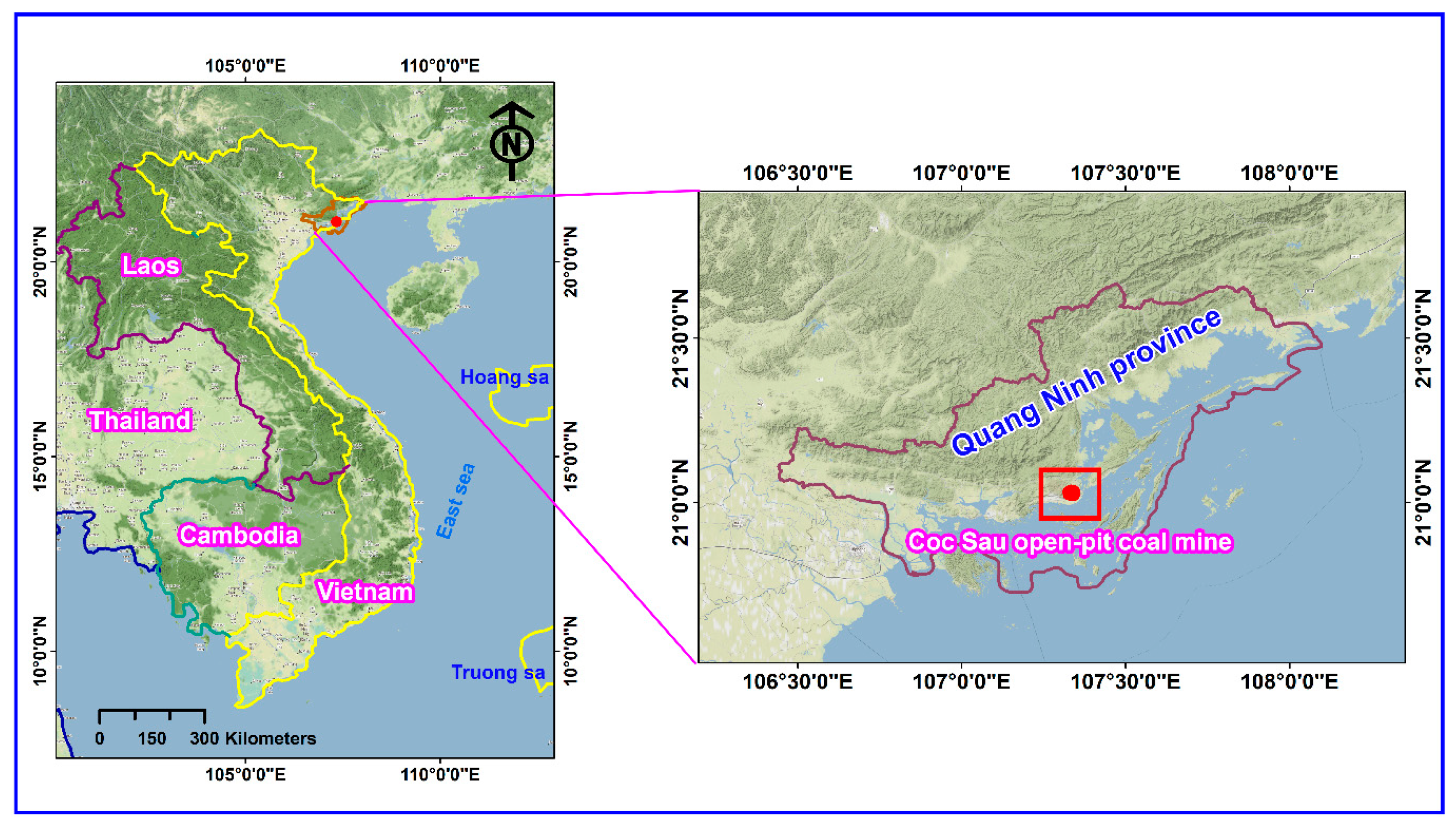
Figure 1. Location of the study site.
Applsci 09 02806 g001
Figure 2. Simplified geological conditions of the Coc Sau open-pit coal mine.
Applsci 09 02806 g002
Figure 3. The distance from the mine to the residential area.
Applsci 09 02806 g003
Figure 4. Data collection at the Coc Sau open-pit coal mine for this study.
Applsci 09 02806 g004
Figure 5. Relationship between input and output variables used in this study.
Applsci 09 02806 g005
Figure 6. The composition of dust particles in drilling operations at the Coc Sau open-pit coal mine. The y-axis depicts the number of counts, and the x-axis represents the energy of the X-rays.
Applsci 09 02806 g006
Figure 7. The database used for predicting drill-induced PM10 concentration in this study.
Applsci 09 02806 g007
Figure 8. Performance of the random forest (RF) model for forecasting PM10 concentration on the training dataset.
Applsci 09 02806 g008
Figure 9. Root-mean-squared error (RMSE) of the classification and regression trees (CART) model with various cp values on the training dataset.
Applsci 09 02806 g009
Figure 10. Performance of the k-nearest neighbors (KNN) model with various k.
Applsci 09 02806 g010
Figure 11. Proposing the PSO-SVR model for estimating PM10 concentration.
Applsci 09 02806 g011
Figure 12. Performance of the PSO-SVR-L model on the training dataset.
Applsci 09 02806 g012
Figure 13. Performance of the PSO-SVR-P model on the training dataset.
Applsci 09 02806 g013
Figure 14. Performance of the PSO-SVR-RBF model on the training dataset.
Applsci 09 02806 g014
Figure 15. Measured versus predicted values of PM10 concentration on the testing dataset.
Applsci 09 02806 g015
Table 1. Summary of works using AI techniques for predicting PM10 concentration and TSP.
No.ReferenceTechniqueObjectiveResult
1Chelani, Gajghate [45]ANNPM10RMSE = 7.9; R2 = 0.89
2McKendry [46]ANNPM10RMSD = 2.21; r = 0.75
3Lal and Tripathy [47]ANNPM10RMSE = 0.0339; d = 0.9969
4Alkasassbeh, Sheta [48]ANNPM10, TSPMSEPM10 = 219.785; MSETSP = 1010.7; MMREPM10 = 0.313; MSETSP = 0.234
5Mishra, Goyal [49]Neuro-fuzzyPM2.5R = 0.72
6Nagesha, Chandar [50]ANNPM10MSE = 0.00606; R2 = 0.96
7Patra, Gautam [51]ANNPM0.23–0.3
PM0.3–0.4
PM0.4–0.5
PM0.5–0.65
PM0.65–0.8
PM0.8–1
PM1–1.6
R = 0.806, 0.852, 0.808, 0.896, 0.698, 0.674, 0.788, respectively
Table 2. Characteristics of the data used.
Elementsd (mm)P (m/min)Wtn (%)S (%)
Min.200.00.16000.2915.20
1st Qua.200.00.21007.8424.70
Median230.00.250011.3827.60
Mean227.30.255811.5727.58
3rd Qua.250.00.290015.3930.10
Max.250.00.410028.1239.20
Elementsρ (gm/cm3)σc (MPa)R (m)PM10 (gm/s)
Min.1.22013.0016.000.148
1st Qua.1.23015.0020.000.329
Median1.24016.0022.000.474
Mean1.24315.9821.630.496
3rd Qua.1.26017.0023.000.646
Max.1.27019.0027.001.306
Note: drilling diameter/diameter of borehole (d), penetration rate of the drill (P), moisture content (Wtn), silt content (S), density of rock mass (ρ), compressive strength (σc), rebound hardness number (R), particulate matter 10 micrometers (PM10).
Table 3. Hyper-parameters of the SVR models with the different kernel functions.
ModelHyper-Parameters
CdγΣ
PSO-SVR-L---
PSO-SVR-P-
PSO-SVR-RBF--
Note: cost (C); degree (d); scale (γ); sigma (σ).
Table 4. The parameters of the PSO-SVR models for estimating PM10 concentration.
ModelHyper-Parameters
Cdγσ
PSO-SVR-L900.792---
PSO-SVR-P509.61120.0014-
PSO-SVR-RBF19.988--0.01
Table 5. Performance indices of the PM10 concentration predictive models.
ModelTrainingTesting
RMSER2RMSER2
RF0.0570.9630.0600.894
CART0.0520.9450.0520.924
KNN0.0740.9040.0670.867
PSO-SVR-L0.0360.9630.0400.954
PSO-SVR-P0.0400.9620.0420.948
PSO-SVR-RBF0.0410.9620.0430.946
Note: The bold type represents the best model. RMSE denotes root-mean-square error; R2 denotes determination coefficient.
Table 6. Important parameters of the models in this study.
ModelPerformanceImportance Parameters
RMSER2dPWtnSρσcR
RF0.0600.8940.0180.8250.9270.0080.0170.7790.013
CART0.0520.9240.0190.8240.9290.0070.0170.7840.012
KNN0.0670.8670.0240.8020.8960.0060.0220.8260.014
PSO-SVR-L0.0400.9540.0180.8250.9750.0060.0180.8170.012
PSO-SVR-P0.0420.9480.0170.8360.9570.0070.0180.8120.013
PSO-SVR-RBF0.0430.9460.0160.8390.9550.0060.0180.8130.013
Note: drilling diameter/diameter of borehole (d), penetration rate of the drill (P), moisture content (Wtn), silt content (S), density of rock mass (ρ), compressive strength (σc), rebound hardness number (R), particulate matter 10 micrometers (PM10), root-mean-squared error (RMSE), determination coefficient (R2).