An Integrated Wildlife Recognition Model Based on Multi-Branch Aggregation and Squeeze-And-Excitation Network

Featured Application

The method proposed in the article can be used for intelligent monitoring and identification of wildlife in the natural environment.

Abstract

Infrared camera trapping, which helps capture large volumes of wildlife images, is a widely-used, non-intrusive monitoring method in wildlife surveillance. This method can greatly reduce the workload of zoologists through automatic image identification. To achieve higher accuracy in wildlife recognition, the integrated model based on multi-branch aggregation and Squeeze-and-Excitation network is introduced. This model adopts multi-branch aggregation transformation to extract features, and uses Squeeze-and-Excitation block to adaptively recalibrate channel-wise feature responses based on explicit self-mapped interdependencies between channels. The efficacy of the integrated model is tested on two datasets: the Snapshot Serengeti dataset and our own dataset. From experimental results on the Snapshot Serengeti dataset, the integrated model applies to the recognition of 26 wildlife species, with the highest accuracies in Top-1 (when the correct class is the most probable class) and Top-5 (when the correct class is within the five most probable classes) at 95.3% and 98.8%, respectively. Compared with the ROI-CNN algorithm and ResNet (Deep Residual Network), on our own dataset, the integrated model, shows a maximum improvement of 4.4% in recognition accuracy.

1. Introduction

Infrared camera-traps are a non-intrusive monitoring method that can monitor wildlife in nature reserves and collect monitoring images without causing disturbance. Fundamental studies, such as rare species detection, species’ distribution evaluation, animal behavior monitoring, and other vital studies [1], are supported by this method. However, traditional analytics of the monitoring images can take a lot of manual labor and time. The automatic wildlife identification method based on deep learning can save time and labor costs, reduce the monitoring cycle of wildlife, and enable timely study of the distribution and living conditions, which can promote effective protection.

The method of automatic learning of represented features from data based on deep learning has effectively improved the performance of target detection [2]. Therefore, deep learning has been used by many researchers for wildlife identification. Kamencay et al. [3] studied the identification methods of principal component analysis, linear discriminant analysis, and local binary mode histogram of wild animal images. The experiment result shows that Local Binary Patterns Histograms (LBPH) are better than Principal Component Analysis (PCA) and Linear Discriminant Analysis (LDA) for small training data sets. Okafor et al. [4] proposed a wildlife identification method based on deep learning and visual vocabulary, which used grayscale color information and different spatial aggregation methods to complete the training process, the accuracy of which reached 99.93%. By incorporating knowledge about object similarities from visual and semantic domains during the transfer process, Tang et al. [5] proposed the object similarity-based knowledge transfer method, which achieved state-of-the-art detection performance using the semi-supervised learning method. Owoeye et al. [6] used the convolutional neural network (CNN) and recurrent neural network (RNN) to recognize the collective activities of a herd of sheep. Despite a deviation in the distribution of herd activity, the collective activities of the herd were accurately identified. Manohar et al. [7] proposed an effective system for animal recognition and classification based on texture features, which obtained the required features from the local appearance and texture of the animals. Furthermore, they classified them by using K nearest neighbor (KNN) and support vector machine. The final accuracy of the KNN algorithm was 66.7%, which was better than Support Vector Machine (SVM). Zhang et al. [8] proposed a method for selecting filters in deep networks using a weak detector and a spatially weighted Fisher vector, and this method achieved superior results in fine-grained identification of birds. However, this method does not adopt an end-to-end structure and it needs to be finely adjusted for the difference of data distribution in the middle part. Liu et al. [9] first used the “you only look once” (YOLO) model to detect wildlife areas, and proposed a two-channel convolutional neural network to identify wildlife, achieving an accuracy of more than 90%. This method needs accurate markings of the positions of the targets, which reduces the efficiency of wildlife recognition. The above studies all detect and identify wildlife under certain conditions, but there are still problems, such as unsatisfactory accuracy, high calibration cost, and high algorithm complexity.

The Deep Residual Network (ResNet) was proposed by He et al. [10]. The 152-layer neural network was successfully trained and won the championship in ILSVRC2015, the error rate of which on Top-5 (when the correct class is within the five most probable classes) was 3.57%, which was an outstanding effect. To simplify the calculation process and reduce the structure parameters, Xie et al. [11] improved the structure of ResNet and proposed a new structure, ResNeXt. Thanks to its excellent performance, it is widely used in target detection, image recognition [12], and other applications [13]. Niki et al. [14] combined the depth residual block with the slice convolution to generate a classification score for a particular food category, achieving an accuracy of 90.27% on the Food-101 data set. Based on the residual block concept, Peng et al. [15] added a branch of attention to the last convolutional layer of each block of the network, which aims to focus on finger micro-gestures and reduce noise from the wrist and background. A better recognition effect was achieved on the holographic 3D micro-gesture database (HoMG). Researchers Nigati et al. [16] used Visual Geometry Group Network (VGGNet) and ResNet to automatically classify high-resolution remote sensing plant community images. The highest classification accuracy of the ResNet model and the VGGNet model were 91.83% and 89.56%, respectively. The ResNet50 model presented better classification results. Koné et al. [17] designed a layered residual network model to address the problem of large histological images and error-prone analysis, and an accuracy of 0.99 in pathological segmentation tests was achieved. Most importantly, the training based on ResNeXt or ResNet is a weakly supervised learning method, which only need image-level annotations. Tang et al. [18] proposed a model enhancing the weakly supervised deformable part-based models (DPMs) by emphasizing the importance of location and size of the initial class-specific root filter, using only image-level annotations. Extensive experimental results proved that the model has competitive final localization performance in weakly supervised object detection.

In summary, weakly supervised training can improve the efficiency of target detection and recognition. As a mature deep convolutional neural network, the deep residual network is widely used in various image classification applications, and it has achieved satisfactory recognition effects. Therefore, an integration model combining Squeeze-and-Excitation network (SENet) and ResNext was utilized to improve the efficiency and accuracy of recognizing large volumes of monitoring images. The rest of this paper is organized as follows. Section 1 reviews the related work of automatic wildlife recognition. Section 2 introduces the structure of a multi-branch aggregation transformation residual network and SENet. Section 3 shows the structure of SE-ResNeXt for wildlife recognition. Section 4 evaluates the performance of the SE-ResNeXt on two different datasets. The conclusions are drawn in Section 5.

2. Related Work

The residual network is a structure based on a convolutional neural network [19]. Compared with the traditional neural network, the key difference of ResNet is the “shortcut connection”, which is realized by directly adding the input to the output. This is equivalent to the fusion of the underlying feature information to the top level, which makes it possible to retain some of the characteristic information of small receptive wild targets. In addition, the problem of “degeneration” of deep neural networks is addressed. When the number of the layers increases, the error rate is correspondingly improved, and the Stochastic Gradient Descent (SGD) optimization becomes more difficult, affecting the learning efficiency of the model. At the same time, the higher the number of layers in the network, the more likely the network can lead to serious gradient disappearance problems. To some extent, this problem can be solved by normalizing initialization and intermediating normalization to ensure the normal convergence of the deeper networks. However, in deeper networks, degradation still exists. In response to the above situation, a residual module is introduced to the deep network to perform “residual learning”. The entire network is simplified to learn the direct residuals of input and output, which greatly reduces the learning objectives and the training complexity.

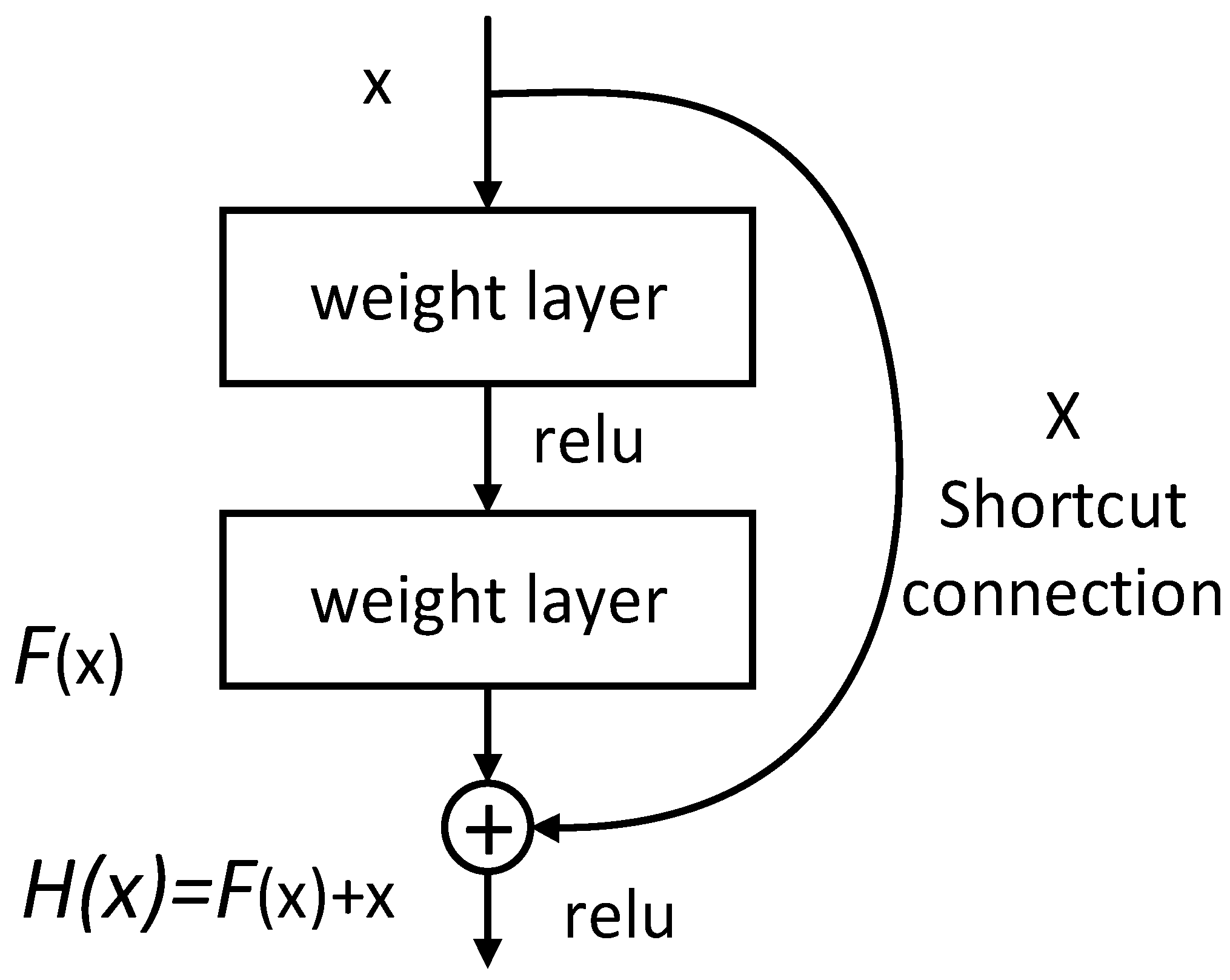
2.1. The Construction of Residual Block

The basic structure of the residual module is shown in Figure 1.

In this figure, x denotes the input and H(x) denotes the desired underlying mapping. The stacked nonlinear layers is expected to fit another mapping of F(x) = H(x) − x. The original mapping is recast into F(x) + x. It is easier to optimize the residual mapping than to optimize the original, unreferenced mapping. In the extreme, if an identity mapping is optimal, it would be easier to push the residual to zero than to fit an identity mapping by a stack of nonlinear layers. The formulation of F(x) + x can be realized by feedforward neural networks with “shortcut connections”. Shortcut connections are those skipping one or more layers. The simple addition can greatly increase the training speed of the model and improve the training results without adding extra parameters or computational complexity.

The residual learning is adopted to each stacked layer. The module is defined as follows.

$$y=F\left(x,\left\{W_i\right\}\right)+x$$

(1)

where x and y denote the input and output of the module respectively. The function $F\left(x,\left\{W_i\right\}\right)$ represents the residual mapping to be learned. The operation F + x is performed by a shortcut connection and element-wise addition. The dimensions of x and F must be equal in Equation (1). If the dimensions are inconsistent, a linear projection Ws shall be performed by the shortcut connections to match the dimensions.

$$y=F\left(x,\left\{W_i\right\}\right)+W_{s}x$$

(2)

The square matrix W_s is only used when matching dimensions.

This residual hopping structure breaks the convention that the output of the traditional neural network n − 1 layer can only give the n layer as an input, so that the output of a certain layer can directly cross several layers as the input of a later layer. In this way, the error rate of the whole learning model will not be improved after superimposing the multi-layer network, which provides feasibility for the extraction and classification of high-level semantic features.

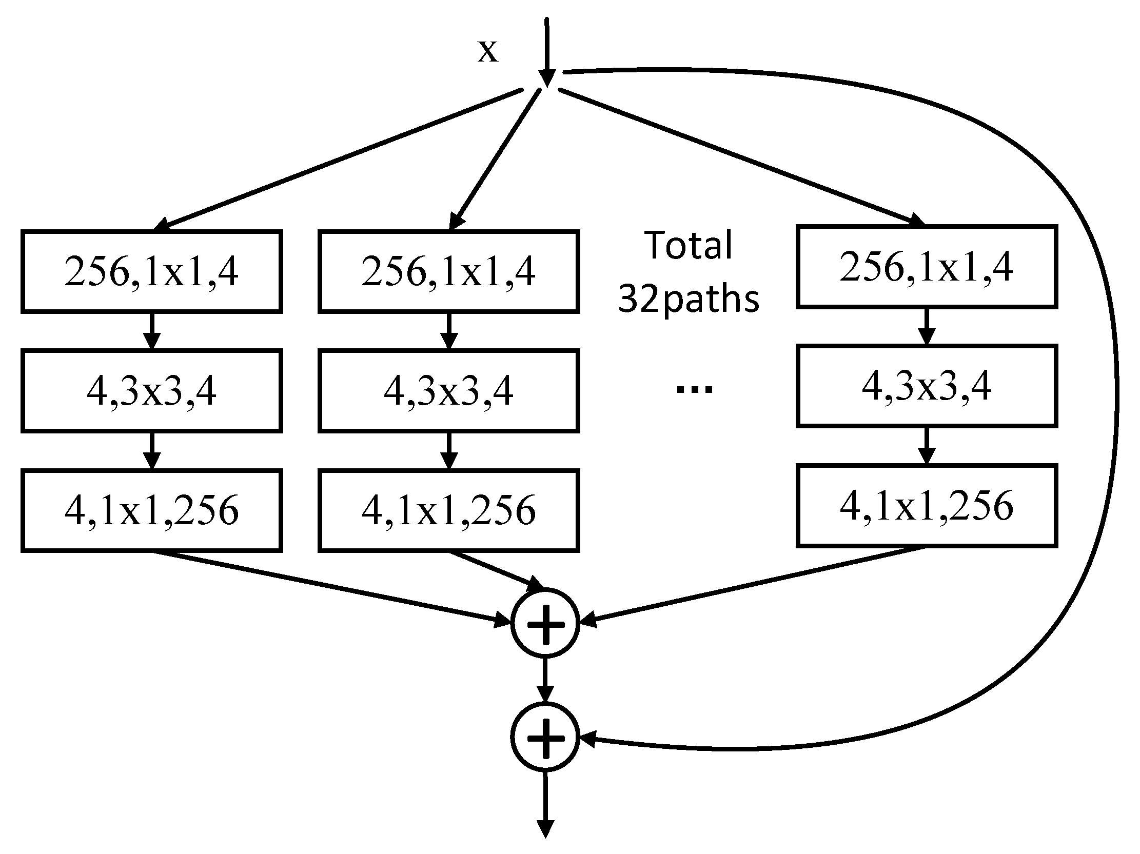
2.2. Multi-Branch Aggregation Transformation Residual Network

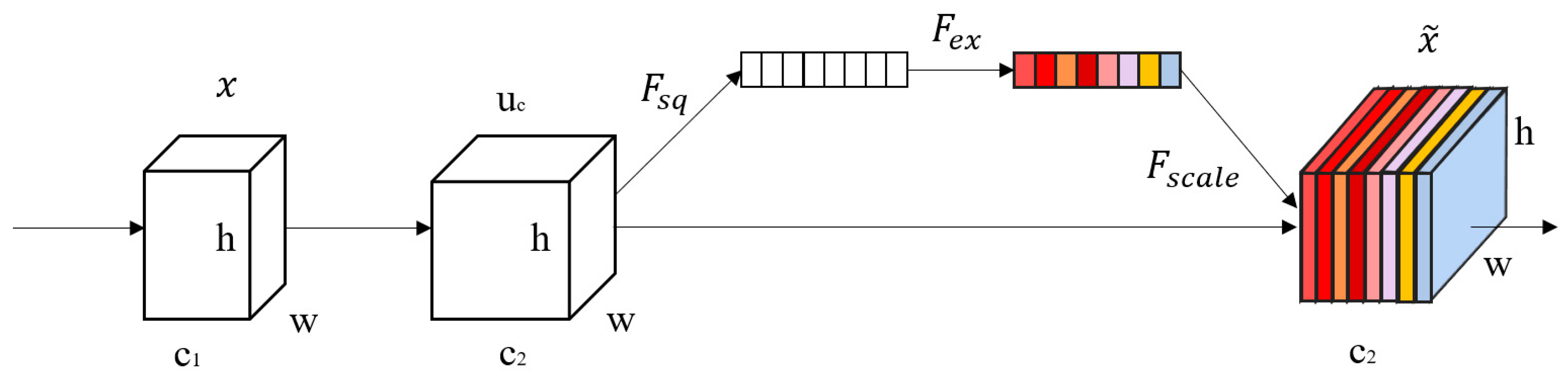
While depth and width keep increasing, they start to induce diminishing returns for existing models. To avoid this problem, this paper adopts a multi-branch aggregation transform residual network called ResNext. The architecture adopts strategy of repeating layers, while exploiting the split-transform-merge strategy in an easy, extensible way. A module in the network performs a set of transformations, each on a low-dimensional embedding, whose outputs are aggregated by summation. This design allows us to extend to any large number of transformations without specialized designs.

The basic unit structure is shown in Figure 2.

Each unit is a bottleneck. Firstly, 1 × 1 convolution is used to compute reductions before other operations. The input feature map is converted into a four-channel feature map. Then a 3 × 3 convolution operation is performed, and next through the 1 × 1 convolution to increase the input channel number to 256. Finally, the feature maps of the 32 branches are aggregated. The structure is a 32 × 4 d structure, where 32 is the new degree of freedom introduced by ResNeXt, called cardinality.

2.3. SENet

SENet is a convolutional neural network structure proposed by Hu et al. [20] in 2017. The structure consists of Squeeze, Excitation, and Reweight. Different from the traditional method of introducing a new spatial dimension for the fusion of feature channels, the network structure adopts a “feature recalibration” strategy to explicitly construct the interdependence between feature channels.

Figure 3 is the structural diagram of the SENet. The number of characteristic channels of input x is c₁, and a feature of the feature channel number c₂ is obtained by a general transformation such as a series of convolutions. Different from the traditional CNN, the following three functions are used to “recalibrate” the previously obtained features.

The first operation is Squeeze. Feature maps obtained by the previous operations are aggregated to produce a channel descriptor. Through this operation, each two-dimensional feature map is compressed by a global average pooling to become a real number, and the output of the c feature maps is a real number column of 1 × 1 × c, which is expressed as in Equation (3) given in [18]:

$${\mathrm{z}}_c=F_{sq}(u_c)=\frac{1}{W\times H}{\displaystyle \sum _{i=1}^W{\displaystyle \sum _{j=1}^H{u}_c(i,j)}}$$

(3)

The next operation is excitation also known as adaptive recalibration. Hu et al. [18] employ a simple gating mechanism with a sigmoid activation to fully capture channel-wise dependencies. This operation makes the model obtain a collection of per-channel modulation weights which are vital for SENet. As follows given in [18]:

$$s=F_{ex}(z,W)=\sigma (g(z,W))=\sigma (W_2\delta (W_{1}z))$$

(4)

where $\sigma$ refers to the Rectified Linear Units (ReLU) [21] function, $W_1\in R^{\frac{C}{\mathrm{r}}\times C}$ and $W_2\in R^{C\times \frac{C}{\mathrm{r}}}$.

Firstly, the feature dimension is reduced by a fully connected layer and activated by ReLU. Then it is brought back to the original dimension by a fully connected layer.

The final operation is to re-scale the feature maps. The $s_c$ obtained through excitation is weighted to the corresponding feature map by multiplication and then the model gets the final output of the block, that is c₂ in Figure 3. The re-calibration of the original feature is completed as in Equation (5) given in [18]:

$${\tilde{x}}_c=F_{scale}(u_c,s_c)=s_c\cdot u_c$$

(5)

where $\tilde{x}=\left[{\tilde{x}}_1,{\tilde{x}}_2,\dots ,{\tilde{x}}_c\right]$ and $F_{scale}(u_c,s_c)$ refers to channel-wise multiplication between the scalar $s_c$ and the feature map $u_c\in R^{H\times W}$.

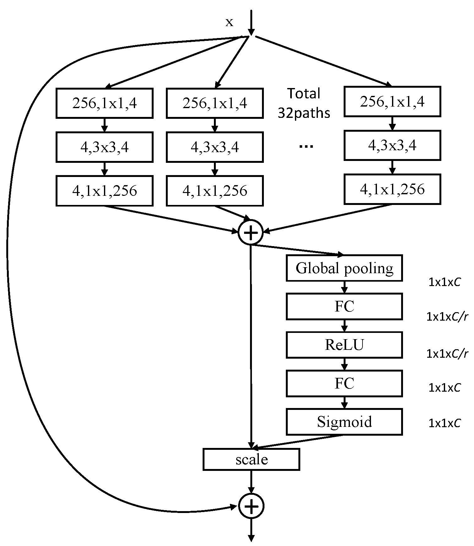
3. The Design of SE-ResNeXt

To conclude the monitoring image features more accurately and adequately, then achieve higher accuracy and efficiency of the automatic recognition, the SENet and multi-branch aggregation transformation are merged and improved to form the SE-ResNeXt structure in this section.

The basic module is shown in Figure 4.

Firstly, the feature of x is extracted and merged by the convolution group in the module, and the feature map, whose channel number is c, is obtained. A Squeeze operation on the feature map is compressed by using global average pooling to obtain a real number column of 1 × 1 × c. Then, the interdependencies between the channels are captured to obtain scale factors through an adaptive recalibration process. Finally, the features are recalibrated through the scale operation.

Table 1. Configuration of the network structure (adapted from a previous study [18]).

Output	ResNet-50 a	SE-ResNeXt-50 a
112 × 112	Conv b, 7 × 7, 64, stride 2
56 × 56	Max pool, 3 × 3, stride 2
	$\left[\begin{array}{l}\mathrm{conv},1\times 1,64\\ \mathrm{conv},3\times 3,64\\ \mathrm{conv},1\times 1,256\end{array}\right]\times 3$	$\left[\begin{array}{l}\mathrm{conv},1\times 1,128\\ \mathrm{conv},3\times 3,128 \mathrm{C}=32\\ \mathrm{conv},1\times 1,256\\ fc,[16,256]\end{array}\right]\times 3$
28 × 28	$\left[\begin{array}{l}\mathrm{conv},1\times 1,128\\ \mathrm{conv},3\times 3,128\\ \mathrm{conv},1\times 1,512\end{array}\right]\times 4$	$\left[\begin{array}{l}\mathrm{conv},1\times 1,256\\ \mathrm{conv},3\times 3,256 \mathrm{C}=32\\ \mathrm{conv},1\times 1,512\\ fc,[32,512]\end{array}\right]\times 4$
14 × 14	$\left[\begin{array}{l}\mathrm{conv},1\times 1,256\\ \mathrm{conv},3\times 3,256\\ \mathrm{conv},1\times 1,1024\end{array}\right]\times 6$	$\left[\begin{array}{l}\mathrm{conv},1\times 1,512\\ \mathrm{conv},3\times 3,512 \mathrm{C}=32\\ \mathrm{conv},1\times 1,1024\\ fc,[64,1024]\end{array}\right]\times 6$
7 × 7	$\left[\begin{array}{l}\mathrm{conv},1\times 1,512\\ \mathrm{conv},3\times 3,512\\ \mathrm{conv},1\times 1,2048\end{array}\right]\times 3$	$\left[\begin{array}{l}\mathrm{conv},1\times 1,1024\\ \mathrm{conv},3\times 3,1024 \mathrm{C}=32\\ \mathrm{conv},1\times 1,2048\\ fc,[128,2048]\end{array}\right]\times 3$
1 × 1	Global average pool, 1000-d fc, softmax

^a ResNet and SE-ResNeXt represent the model structure, 50 represents the number of layers. ^b Conv represents convolutional layer.

shows the network structure configuration of ResNet-50 and SE-ResNeXt-50.

The numbers following the fc indicate C/r and C, respectively. In Table 1, all basic modules of two network structures consist of three convolution layers with 16 modules. The first and the last are 1 × 1 convolution layers and the middle one is a 3 × 3 convolution layer. The difference between the two network structures is that a convolution group rather than a single convolution block exists in the SE-ResNeXt-50 module. Additionally, each module has a full connection operation. This paper will evaluate the SE-ResNeXt model based on the above network structure in the following section.

4. Results and Discussion

Experiments for our study are performed on the paddlepaddle platform. The experiment system environment is Ubuntu 16.04 and the programming language is python. The hardware configuration encompasses an E5-2620 Central Processing Unit (CPU) and GTX1080ti Graphics Processing Unit (GPU).

4.1. Comparative Experiments of Different Models on our Own Dataset

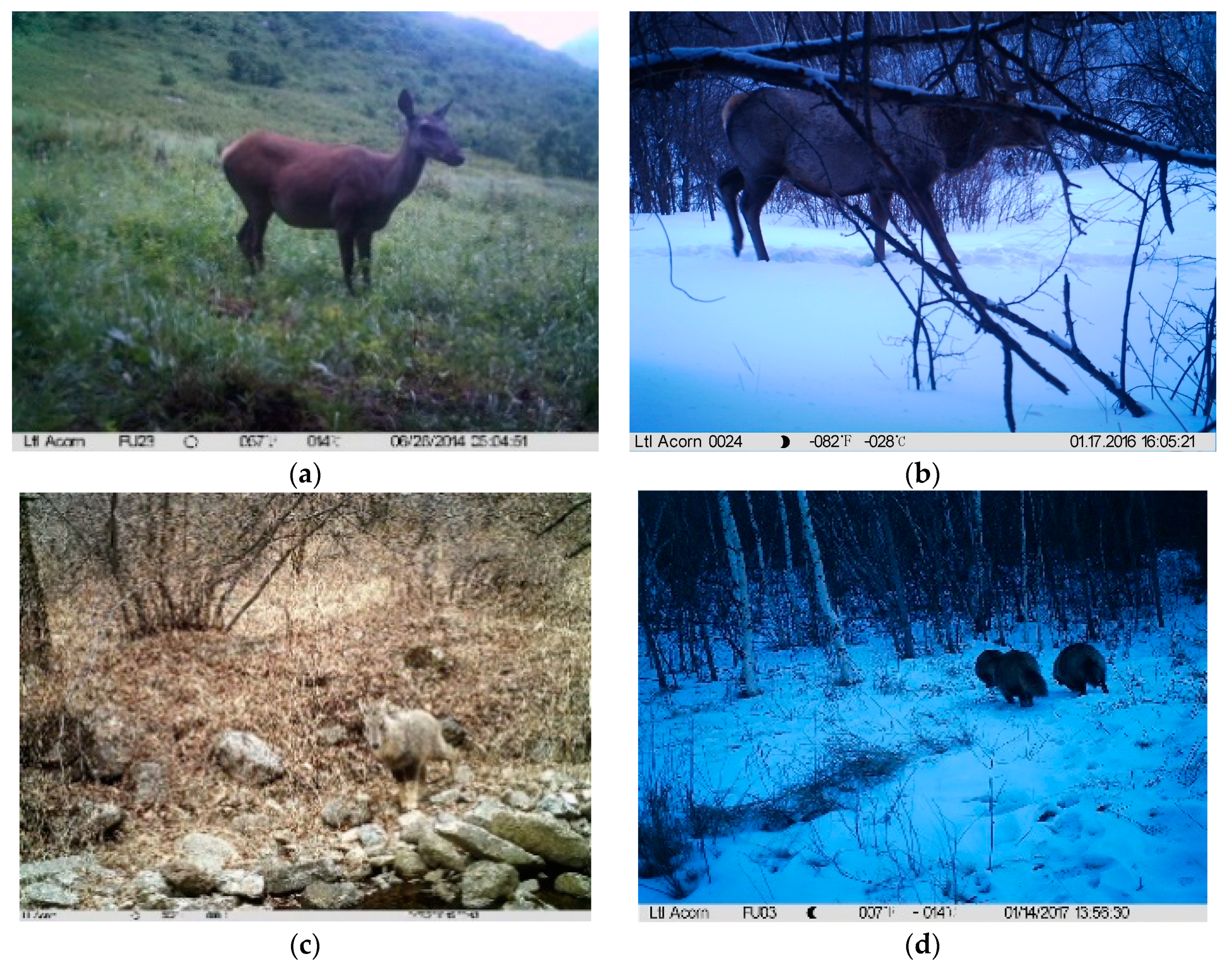
4.1.1. Our Own Dataset

In this section, the images of wildlife were acquired by infrared camera in the Saihanwula National Nature Reserve in Inner Mongolia from 2010 to 2019 [22]. Thousands of wildlife monitoring images were obtained and a sample library of wildlife monitoring images was established. The monitoring images consist of 24-bit RGB true color images with a resolution of 2560 × 1920. In this paper, five common terrestrial protected species [23] were selected, including Red Deer, Goral, Roe Deer, Lynx, and Badger.

Table 2. Wildlife image sample database.

Species	Red Deer	Goral	Roe Deer	Lynx	Badger
Daytime	2822	1027	1698	301	292
Dark	1782	639	839	120	146
Number of Images	4604	1666	2537	421	438

shows the image numbers for the five species in the image sample library. Figure 5 shows a sample of wildlife monitoring images.

Figure 5a shows the monitoring image of the red deer, in which the individual target is complete and its outline is clear. However, high-quality images are few in the dataset, as most images have various defects, such as obstructions (Figure 5b), indistinguishable backgrounds (Figure 5c), and targets being too far away (Figure 5d). When such images are artificially marked, subjectivity will affect the accuracy of feature extraction, affecting the characteristic learning ability of the model.

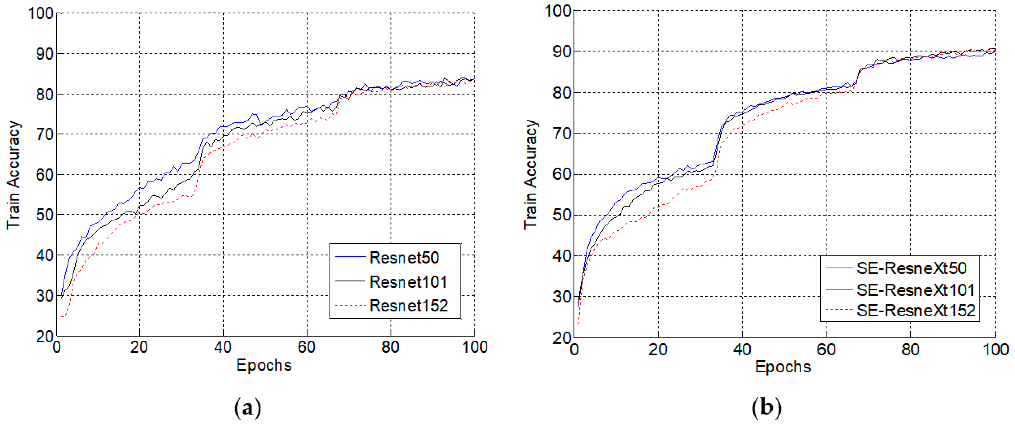
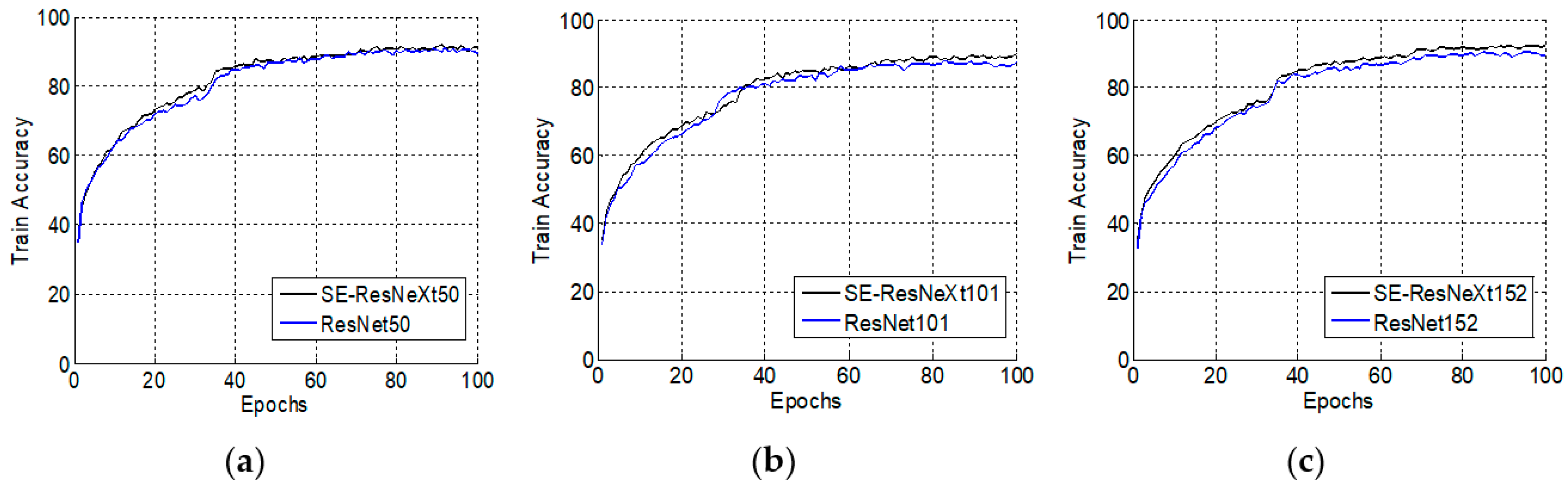
4.1.2. Comparison Experiments of ResNet and SE-ResNeXt in Different Numbers of Layers

Based on our own dataset, ResNet and SE-ResNeXt with layers of 50, 101, and 152 were used for comparison experiments. The experimental learning rates in this section were set to 0.1 and 0.01, respectively. The comparison work is conducted by analyzing the training results from two groups of experiments. One group is set with the same number of layers under different structures. The other is set with different numbers of layers under the same structure. Figure 6 shows the results of the comparison experiments where the number of layers is different.

As shown in the above figures, the maximum training accuracy of ResNet is approximately 83.6%, regardless of the number of layers, which is the same as the SE-ResNeXt with different layers. The difference is that the maximum accuracy of SE-ResNeXt training is higher than ResNet, which is close to 90.6%, indicating that the training of SE-ResNeXt has better recognition performance. Even if the final accuracy is similar, the training process is different for models with different layers. Before 70 epochs, the higher the number of layers, the lower the accuracy of training when the number of iterations is the same. This is because the model has more parameters when the number of layers increases, so it needs more iterations to obtain higher precision.

Figure 7 and Figure 8 show the training accuracy variations with epoch changes when the learning rates are 0.1 and 0.01, respectively. When the learning rate is 0.1, the train accuracy of SE-ResNeXt is higher than that of ResNet throughout the training process, regardless of the number of layers. Moreover, as the epoch increases, the difference in accuracy also increases. When the learning rate is reduced to 0.01, the difference decreases. In the process of training, there is almost no difference between the SE-ResNeXt and the ResNet when the number of layers is 50. As the number of layers increases, the difference between SE-ResNeXt and ResNet increases marginally.

Table 3. Test accuracy of six models.

Layers	50		101		152
Model	ResNet [10]	SE-ResNeXt	ResNet [10]	SE-ResNeXt	ResNet [10]	SE-ResNeXt
lr = 0.01	0.906	0.935	0.898	0.935	0.908	0.921
lr = 0.1	0.879	0.919	0.899	0.929	0.881	0.925

displays the test accuracy of the six models in the two sets of experiments. It can be observed that the accuracy of 0.01 learning rate is higher than that of 0.1 learning rate for all six models. In addition, the learning rate has a significantly greater impact on ResNet than the impact on SE-ResNeXt. In two experiments with different learning rates, the accuracy differences of ResNet50 and ResNet152 both reached 2.7%, while the accuracy difference of SE-ResNeXt was only 1.6%. This shows that reducing the learning rate is beneficial for improving the recognition accuracy. At the same time, it can be seen intuitionally from the table that the test accuracy of SE-ResNeXt is always higher than that of ResNet when the models have the same number of layers. The maximum difference reaches 4.4%. From the table, it can be concluded that the training of SE-ResNeXtn101 achieves the best test results when the learning rate is 0.01.

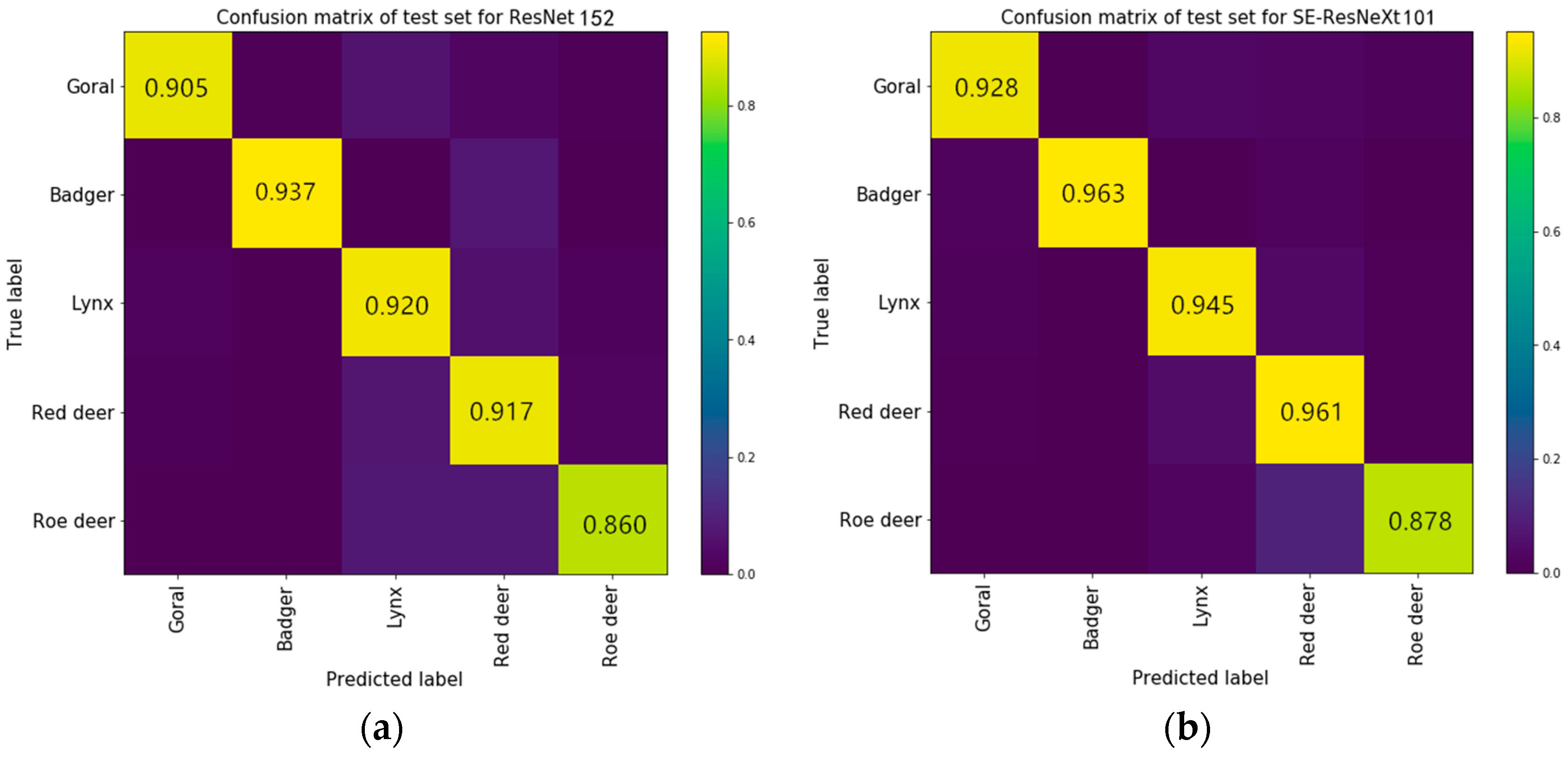
4.1.3. Comparison Experiments of Accuracy for Each Category

To further validate the advantages of the integrated model, the accuracy of each category is compared in this section. According to the above experiments, ResNet152 and SE-ResNeXt101, which achieve the highest test accuracy in the corresponding structures, were compared. The confusion matrix is used to compare the accuracy for each category of the two models.

Figure 9a,b are the confusion matrices of test sets for ResNet152 and SE-ResNeXt101, respectively. The values on the diagonal represent the accuracy of the model for recognizing Goral, Badger, Lynx, Red Deer, and Roe Deer. The more yellow the color of the matrix, the better the model recognizes the corresponding species.

SE-ResNeXt101 has higher recognition accuracy for five species than ResNet152 and the maximum difference is 4.4%. For the two models, the performance of recognizing Roe Deer is worse than other categories. This is because Roe Deer resembles Red Deer, but the number of Roe Deer images is only half the number of Red Deer and the image quality is lower than that of Red Deer. When identifying Red Deer, with the help of so many high-quality images, the accuracy of SE-ResNeXt101 is much higher than that of ResNet152. The results prove that SE-ResNeXt can achieve better performance in recognition tasks on our own dataset.

4.2. Comparative Experiment with Existing ROI-CNN Algorithm

Liu et al. proposed an automatic recognition algorithm for wildlife based on ROI-CNN [9], which achieved a recognition accuracy of 91.2%. The algorithm firstly extracts the region of interest from the images and obtains the ROI image. Then, the model is imported for the training process. There is a large amount of work in the image labeling step, which is regarded as a strong supervision study. To verify the advantages of the integration model, the same training samples are used and the test accuracy of each network structure is shown in

Table 4. Comparison of Test accuracy.

Model	ROI-CNN [9]	ResNet-50 [10]	ResNet-101 [10]	ResNet-152 [10]	SE-50 *	SE-101	SE-152
Test acc	0.912	0.902	0.870	0.835	0.906	0.902	0.914

* SE represents SE-ResNeXt which was proposed.

.

From Table 4, ResNet50, SE-ResNeXt50, and SE-ResNeXt101 perform slightly worse on the same sample than the ROI-CNN algorithm, but the accuracies are all above 90%. The test accuracy of SE-ResNeXt152 reaches 91.4%, which is slightly higher than Liu’s recognition algorithm. Considering the labor and time cost, manual does is not need to be performed during using our integrated model, so the recognition efficiency of the model is better than that of Liu.

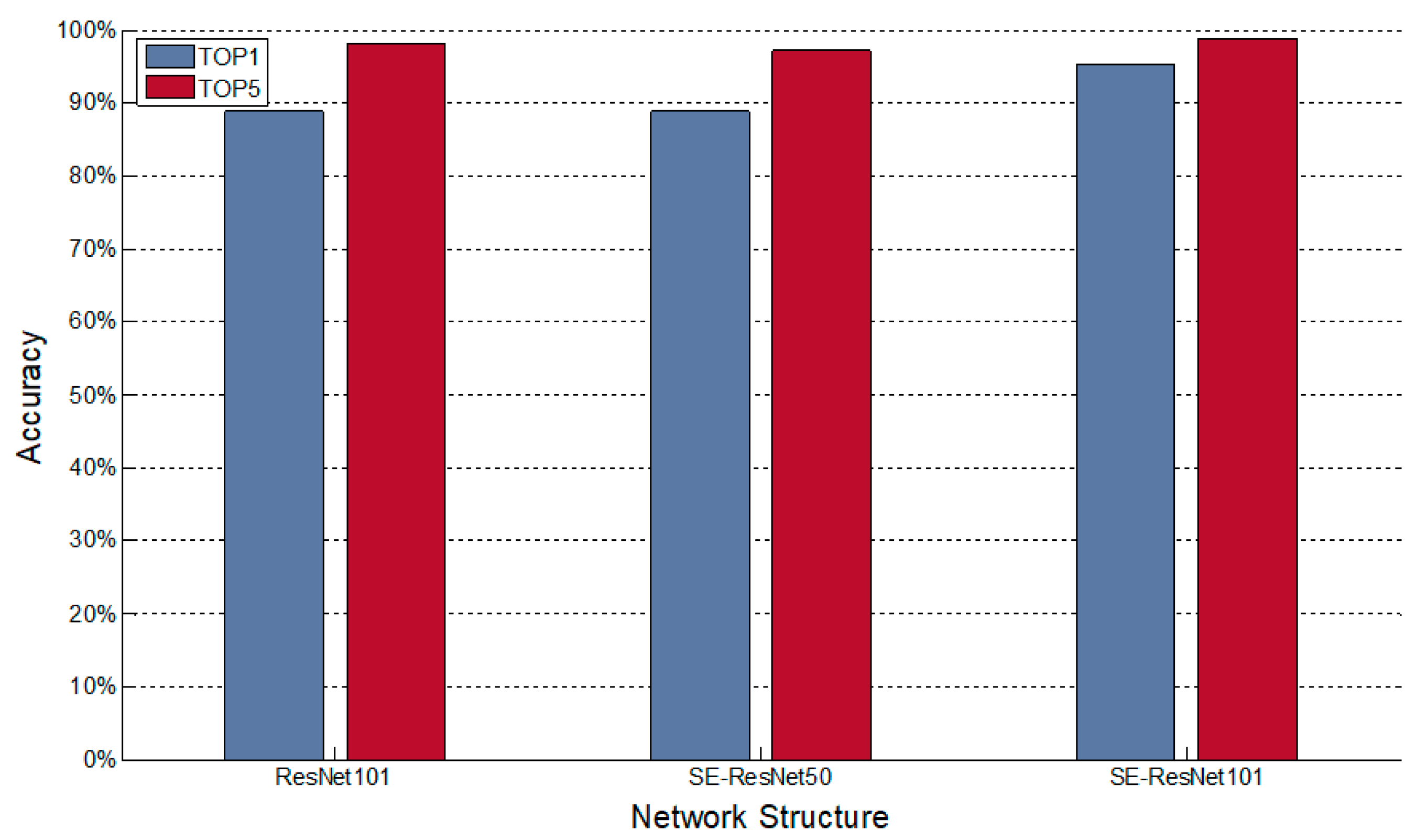
4.3. Comparative Experiments with Snapshot Serengeti Dataset

To further validate the validity of the model, the experiments on a public dataset called Snapshot Serengeti dataset [24] was conducted. It was acquired with 225 camera-traps placed in Serengeti National Park, Tanzania. More than one million sets of pictures were acquired, and each set contains 1–3 photographs. This dataset allows the computer science community to study and overcome the challenges presented in camera trapping frameworks. Additionally, it also helps ecology researchers and educators in their camera-trap studies. In this work, 26 classes were selected form the dataset for recognition (they are listed in

Table 5. Set of species selected from the Snapshot Serengeti dataset.

Species	# Images	Species	# Images
Wildebeest	212,973	Lion, female and cub	8773
Zebra	181,043	Eland	7395
Thomson’s gazelle	116,421	Topi	6247
Buffalo	34,684	Baboon	4618
Human	26,557	Reedbuck	4141
Elephant	25,294	Dik dik	3364
Guinea fowl	23,023	Cheetah	3354
Giraffe	22,439	Hippopotamus	3231
Impala	22,281	Lion male	2413
Warthog	22,041	Kori Bustard	2042
Grants gazelle	21,340	Ostrich	1945
Hartebeest	15,401	Secretary bird	1302
Spotted hyena	10,242	Jackal	1207

).

Gomez-Villa et al. [25] adopted six very deep convolutional neural networks (ConvNets) to train the Snapshot Serengeti dataset and obtained satisfactory results. The six models are AlexNet [26], VGG Net [27], GoogLenet [28], ResNet-50, ResNet-101, and ResNet-152, which are the state-of-the-art in object recognition. Accuracy in the validation set is used as a performance metric. Top-1 (when the correct class is the most probable class) and Top-5 (when the correct class is within the five most probable classes) accuracies are presented to show how well the model performs in ranking possible species.

The best results in Gomez-Villa’s experiments were obtained using ResNet-101, showing 88.9% for Top-1 and 98.1% for Top-5. Using the same dataset, this paper employs SE-ResNeXt50 and SE-ResNeXt101 to compare with Gomez-Villa’s best results. Figure 10 shows the results of experiments, including Top-1 and Top-5 results alongside each experiment.

The results reach an accuracy of 88.8% and 97.1% for Top-1 and Top-5 respectively when the model is SE-ResNeXt50. When the model is SE-ResNeXt101, the results are 95.3% and 98.8% for Top-1 and Top-5 respectively.

Figure 10 shows that the Top-1 and Top-5 of SE-ResNeXt50 have a very subtle difference from those of ResNet101. When trained with SE-ResNeXt101, the accuracy of Top-1 reaches 95.3%, 6.4% higher than that of ResNet101. The value of Top-5 is also slightly higher than that of ResNet101, which proves that SE-ResNeXt performs better than other state-of-the-art models in object recognition, when using the same dataset.

Table 6. The accuracy results of each species.

Species	SE-ResNeXt101	ResNet-101	Species	SE-ResNeXt101	ResNet-101
Wildebeest	91.7	93.1	Lion, female and cub	92.8	83.3
Zebra	96.3	99.5	Eland	97.5	87.5
Thomson’s gazelle	94.5	71.6	Topi	93.1	95.8
Buffalo	97.7	83.3	Baboon	94.8	98.3
Human	99.8	99.1	Reedbuck	93.3	95.0
Elephant	96.8	90.4	Dik dik	94.6	75.8
Guinea fowl	94.1	99.5	Cheetah	94.7	97.0
Giraffe	94.8	96.6	Hippopotamus	97.6	94.1
Impala	98.3	92.0	Lion male	93.5	77.0
Warthog	95.0	98.0	Kori Bustard	94.9	97.9
Grants gazelle	96.2	65.0	Ostrich	92.4	94.1
Hartebeest	93.8	97.5	Secretary bird	92.9	95.4
Spotted hyena	98.9	85.4	Jackal	97.8	92.4

compares the accuracy of each species using the ResNet-101 in Alexander Gomez Villa’s experiments and the SE-ResNeXt101 in this paper.

Table 6 shows that SE-ResNeXt101 has an accuracy of more than 90% for all 26 species. The lowest accuracy is 91.7% on Wildebeest and the highest is 99.8% on Human. As for ResNet-101, the lowest accuracy is 65% on Grants gazelle and the highest is 99.5% on Guinea fowl. For Grants gazelle, the accuracy of SE-ResNeXt101 reaches 96.2%, surpassing that of ResNet-101. According to statistics, the average recognition accuracies of SE-ResNeXt101 and ResNet-101 for 26 species are 95.3% and 88.9%, respectively. It is shown that when the species characteristics are obvious, for example Giraffe and Human, the performance of the two models is similar. In thirteen classes, the SE-ResNeXt101 outperformed the ResNet-101 and the maximum difference reached 31.2% when recognizing Grants gazelle. The color of the Grants gazelle’s hide is similar to that of the background, which makes the recognition more difficult. Similarly, when an identification problem is related to fine-grained classification, for example Lion female and male, the performance of ResNet-101 is obviously poor and the accuracy of SE-ResNeXt101 is still above 90%.

From the above results and discussions, it is concluded that the SE-ResNeXt can obtain the differential characteristics of the wildlife monitoring images through the multi-branch aggregation and “feature recalibration” strategy, which can improve recognition performance without marking the locations of wildlife. Better experimental results are obtained on different datasets, which indicates that the integrated model has better generalization capabilities and performs more stably in recognition.

5. Conclusions

In this paper, an integrated model based on ResNeXt and SENet is employed to realize automatic identification of wildlife. This model combines multi-branch aggregation and a Squeeze and Excitation structure, which can automatically acquire the importance of the feature channel and extract the important features more efficiently, without increasing computational complexity. The model is evaluated on two different datasets in three sets of experiments, with the results showing that the performance of SE-ResNeXt is the best. In the identification experiments of our own wildlife database, the highest recognition accuracy of SE-ResNeXt reached 93.5%. In the experiment on the Serengeti dataset, SE-ResNeXt also outperformed ResNet101, especially in species without or lacking obvious characteristics. Compared with the existing recognition algorithm based on marking locations of wildlife, the SE-ResNeXt can slightly improve the recognition accuracy without labeling images. To conclude, SE-ResNeXt outperforms other state-of-the-art methods in automatic recognition of wildlife monitoring images. Moreover, it improves the efficiency of automatic recognition of wildlife by reducing the location marking workload, which greatly shortens the processing cycle of monitoring data and improves the intelligence level of wildlife protection.

References

1. O’Connell, A.F.; Nichols, J.D.; Karanth, K.U. Camera Traps in Animal Ecologym; Springer: Tokyo, Japan, 2011. [Google Scholar]
2. Jiang, J.; Xu, H.; Zhang, S. Object Detection Algorithm Based on Multiheaded Attention. Appl. Sci. 2019, 9, 1829. [Google Scholar] [CrossRef]
3. Kamencay, P.; Trnovszky, T.; Benco, M.; Hudec, R.; Sykora, P.; Satnik, A. Accurate wild animal recognition using PCA, LDA and LBPH. In Proceedings of the 2016 IEEE ELEKTRO, Strbske Pleso, Slovakia, 16–18 May 2016; pp. 62–67. [Google Scholar]
4. Okafor, E.; Pawara, P.; Karaaba, F. Comparative Study Between Deep Learning and Bag of Visual Words for Wild-Animal Recognition. In Proceedings of the IEEE Symposium Series on Computational Intelligence, Athens, Greece, 6–9 December 2016; pp. 1–8. [Google Scholar]
5. Tang, Y.; Wang, J.; Gao, B.; Dellandréa, E.; Gaizauskas, R.; Chen, L. Large scale semi-supervised object detection using visual and semantic knowledge transfer. In Proceedings of the IEEE Conference on Computer Vision and Pattern Recognition, Las Vegas, NV, USA, 27–30 June 2016; pp. 2119–2128. [Google Scholar]
6. Owoeye, K.; Hailles, S. Online Collective Animal Movement Activity Recognition. In Proceedings of the Workshop on Modeling and Decision-Making in the Spatiotemporal Domain. 32nd Conference on Neural Information Processing Systems, Montreal, QC, Canada, 7 December 2018. [Google Scholar]
7. Manohar, N.; Subrahmanya, S.; Bharathi, R.K.; YH, S.K.; Kumar, H. Recognition and classification of animals based on texture features through parallel computing. In Proceedings of the 2016 Second International Conference on Cognitive Computing and Information Processing, Mysore, India, 12–13 August 2016; pp. 1–5. [Google Scholar]
8. Zhang, X.; Xiong, H.; Zhou, W.; Lin, W.; Tian, Q. Picking deep filter responses for fine-grained image recognition. In Proceedings of the IEEE Conference on Computer Vision and Pattern Recognition, Las Vegas, NV, USA, 27–30 June 2016; pp. 1134–1142. [Google Scholar]
9. Liu, W.; Li, A.; Zhang, J. Automatic identification of terrestrial wildlife in Saihanwula National Nature Reserve based on ROI-CNN. J. Beijing For. Univ. 2018, 40, 124–131. [Google Scholar]
10. He, K.; Zhang, X.; Ren, S.; Sun, J. Deep residual learning for image recognition. In Proceedings of the IEEE Conference on Computer Vision and Pattern Recognition, Las Vegas, NV, USA, 27–30 June 2016; pp. 770–778. [Google Scholar]
11. Xie, S.; Girshick, R.; Dollár, P.; Tu, Z.; He, K. Aggregated residual transformations for deep neural networks. In Proceedings of the IEEE Conference on Computer Vision and Pattern Recognition, Honolulu, HI, USA, 21–26 July 2017; pp. 1492–1500. [Google Scholar]
12. Mcallister, P.; Zheng, H.; Bond, R. Combining deep residual network features with supervised machine learning algorithms to classify diverse food image datasets. Comput. Biol. Med. 2018, 95, 217–233. [Google Scholar] [CrossRef] [PubMed]
13. Zhang, K.; Zhang, H.; Zhou, H. Zebrafish Embryo Vessel Segmentation Using a Novel Dual ResUNet Model. Comput. Intell. Neurosci. 2019, 2019, 8214975. [Google Scholar] [CrossRef]
14. Martinel, N.; Foresti, G.L.; Micheloni, C. Wide-slice residual networks for food recognition. In Proceedings of the IEEE Winter Conference on Applications of Computer Vision, Lake Tahoe, NV, USA, 12–15 March 2018; pp. 567–576. [Google Scholar]
15. Peng, M.; Wang, C.; Chen, T. Attention Based Residual Network for Micro-Gesture Recognition. In Proceedings of the IEEE International Conference on Automatic Face & Gesture Recognition, Xi’an, China, 15–19 May 2018; pp. 790–794. [Google Scholar]
16. Nigati, K.; Shi, Q.; Liu, S.; Biloli, Y.; Li, H. Automatic classification method of oasis plant community in desert hinterland based on VGGNet and ResNet model. J. Agric. Mach. 2019, 50, 217–225. [Google Scholar]
17. Koné, I.; Boulmane, L. Hierarchical ResNeXt Models for Breast Cancer Histology Image Classification. In Proceedings of the International Conference Image Analysis and Recognition, Póvoa de Varzim, Portugal, 27–29 June 2018; pp. 796–803. [Google Scholar]
18. Tang, Y.; Wang, X.; Dellandréa, E. Weakly supervised learning of deformable part-based models for object detection via region proposals. IEEE Trans. Multimed. 2016, 19, 393–407. [Google Scholar] [CrossRef]
19. Yunlong, Y.; Fuxian, L. A Two-Stream Deep Fusion Framework for High-Resolution Aerial Scene Classification. Comput. Intell. Neurosci. 2018, 2018, 8639367. [Google Scholar]
20. Hu, J.; Shen, L.; Sun, G. Squeeze-and-excitation networks. In Proceedings of the IEEE Conference on Computer Vision and Pattern Recognition, Salt Lake City, UT, USA, 19–21 June 2018; pp. 7132–7141. [Google Scholar]
21. Nair, V.; Hinton, G.E. Rectified linear units improve restricted boltzmann machines. In Proceedings of the 27th International Conference on Machine Learning, Haifa, Israel, 21–24 June 2010; pp. 807–814. [Google Scholar]
22. Chen, S.; Hu, C.; Zhang, J. Design of Wildlife Image Monitoring System Based on Wireless Sensor Networks. Mod. Manuf. Technol. Equip. 2017, 3, 64–66. [Google Scholar]
23. Na, L. Nature Monitoring on Wildlife Biodiversity at Saihanwula National Nature Reserve; Beijing Forestry University: Beijing, China, 2011. [Google Scholar]
24. Swanson, A.; Kosmala, M.; Lintott, C. Snapshot Serengeti, high-frequency annotated camera trap images of 40 mammalian species in an African savanna. Sci. Data 2015, 2, 150026. [Google Scholar] [CrossRef] [PubMed] [Green Version]
25. Villa, A.G.; Salazar, A.; Vargas, F. Towards automatic wild animal monitoring: Identification of animal species in camera-trap images using very deep convolutional neural networks. Ecol. Inform. 2017, 41, 24–32. [Google Scholar] [CrossRef] [Green Version]
26. Krizhevsky, A.; Sutskever, I.; Hinton, G.E. Imagenet classification with deep convolutional neural networks. In Advances in Neural Information Processing Systems; Massachusetts Institute of Technology Press: Cambridge, MA, USA, 2012; pp. 1097–1105. [Google Scholar]
27. Simonyan, K.; Zisserman, A. Very Deep Convolutional Networks for Large-Scale Image Recognition. In Proceedings of the 2015 International Conference on Learning Representations (ICLR 2015), San Diego, CA, USA, 7–9 May 2015. [Google Scholar]
28. Szegedy, C.; Liu, W.; Jia, Y.; Sermanet, P.; Reed, S.; Anguelov, D.; Erhan, D.; Vanhoucke, V.; Rabinovich, A. Going deeper with convolutions. In Proceedings of the IEEE Conference on Computer Vision and Pattern Recognition, Boston, MA, USA, 7–12 June 2015. [Google Scholar]
Figure 1. A basic block of ResNet (adapted from a previous study [9]).
Applsci 09 02794 g001
Figure 2. A block of ResNext with cardinality = 32 (adapted from [10]).
Applsci 09 02794 g002
Figure 3. Structure diagram of SE block (adapted from [18]).
Applsci 09 02794 g003
Figure 4. Structure diagram of SE-ResNeXt block.
Applsci 09 02794 g004
Figure 5. Wildlife monitoring image: (a) Red deer; (b) Red deer; (c) Goral; (d) Badger.
Applsci 09 02794 g005
Figure 6. Variations of train accuracy with epoch changes (lr = 0.1). (a) The model of ResNet; (b) The model of SE-ResNeXt.
Applsci 09 02794 g006
Figure 7. Variations of train accuracy with epoch changes (lr = 0.1). (a) The number of layers is 50; (b) The number of layers is 101; (c) The number of layers is 152.
Applsci 09 02794 g007
Figure 8. Variations of train accuracy with epoch changes (lr = 0.01). (a) The number of layers is 50; (b) The number of layers is 101; (c) The number of layers is 152.
Applsci 09 02794 g008
Figure 9. Confusion matrices of different models: (a) Confusion matrix of ResNet-152; (b) Confusion matrix of SE-ResNeXt-101.
Applsci 09 02794 g009
Figure 10. Experiments for the Snapshot Serengeti dataset.
Applsci 09 02794 g010