Maximization of Eigenfrequency Gaps in a Composite Cylindrical Shell Using Genetic Algorithms and Neural Networks

Abstract

This paper presents a novel method for the maximization of eigenfrequency gaps around external excitation frequencies by stacking sequence optimization in laminated structures. The proposed procedure enables the creation of an array of suggested lamination angles to avoid resonance for each excitation frequency within the considered range. The proposed optimization algorithm, which involves genetic algorithms, artificial neural networks, and iterative retraining of the networks using data obtained from tentative optimization loops, is accurate, robust, and significantly faster than typical genetic algorithm optimization in which the objective function values are calculated using the finite element method. The combined genetic algorithm–neural network procedure was successfully applied to problems related to the avoidance of vibration resonance, which is a major concern for every structure subjected to periodic external excitations. The presented examples illustrate a combined approach to avoiding resonance through the maximization of a frequency gap around external excitation frequencies complemented by the maximization of the fundamental natural frequency. The necessary changes in natural frequencies are caused only by appropriate changes in the lamination angles. The investigated structures are thin-walled, laminated one- or three-segment shells with different boundary conditions.

1. Introduction

For many years, composites have been used for a variety of applications, such as mechanical, aerospace, and civil engineering structures [1,2,3]. However, the dynamic behavior of composite structures has not been widely investigated: composite structures are slender and light compared with steel and concrete structures, and their dynamic behavior may be entirely different. Understanding this behavior is crucial to the effective application of composite materials in structural engineering [1,4,5,6]. Thus, it is very important to study the dynamic behavior of composite structures in response to changes in material-specific factors (e.g., lamination fiber angles). The structural design process, demand, and the reliability of numerical analysis usually require the optimization of the shape, size, and/or placement of fibers within the material. However, this approach increases the difficulty and complexity of the design process [7] since the design of optimized composite laminate is combined with the search for the best fiber orientation in each layer of composite material. The optimization procedure of laminated composite structures is usually more complex than the one associated with isotropic material structures because of the large number of variables involved and the intrinsic anisotropic behavior of individual layers [8,9].

In optimization problems associated with the design of a composite structure, two scenarios are possible [7,10]: (i) a constant–stiffness design in which the lamination parameters are constant over the whole domain; (ii) a variable–stiffness design in which the lamination parameters may vary in a continuous manner over the domain. The constant–stiffness design scenario is simpler than the variable–stiffness design since there are generally fewer design variables involved [7]. In this study, a constant–stiffness design is applied for a one-segment shell structure, in which the same stacking layup is used over the whole structure, and a variable–stiffness design is applied for a three-segment shell, in which a different stacking layup is used in segments.

In many engineering problems involving dynamic phenomena, the optimization of selected parameters is necessary. Such optimization is usually performed through the minimization or maximization of a carefully selected objective function that describes the distance of particular structure parameters from their desired values (e.g., overall mass, strength, or fundamental natural frequency). The objective function is usually repeatedly solved during the optimization procedure. Moreover, the application of first-order optimization algorithms also involves derivatives of the objective function. In composite laminate design, the precise calculation or even approximation of objective function derivatives is often computationally costly or, in some cases, even impossible. One of the advantages of direct search algorithms (or zero-order optimization algorithms, e.g., Genetic Algorithms, GAs) is that they require only objective function values; no information about the gradient of the objective function is necessary. The single calculation of the objective function is neither difficult nor time-consuming. However, it is extremely computationally demanding when it has to be repeated thousands of times (e.g., when a zero-order search algorithm is applied). Artificial Neural Networks (ANNs) are employed to reduce this demand [11,12]. The task of objective function calculation is herein improved and accelerated by using ANN as a tool to replace the Finite Element Method (FEM) for the prediction of dynamic parameters. The authors of [13] considered a reliability problem for laminated four-ply composite plates in free vibration. The design variables were the material properties, stacking sequence, and thickness of the plies, and the goal of the procedure was to obtain a fundamental natural frequency that was higher than the assumed excitation frequency. The application of neural networks shortened the computation time in the considered problem by more than 40%. Neural networks, trained and tested in advance with FE data almost instantly provide their precise prediction from a big set of candidate solutions, and a GA optimization procedure involving ANNs is thus highly efficient and robust.

In the proposed technique, GA was included to solve the optimization task because functions that describe the dynamic parameters to be optimized have several variables and usually a great number of minima. GA ignores potential local minima and leads to the best solution. This paper presents the maximization of the fundamental natural frequency by determining the optimal fiber orientation in a cylindrical shell’s layers of composite material. The lamination fiber angles are treated as constrained variables that are either continuous or discrete. In the context of improving anti-resonance performance, the maximization of the natural frequency of a structure is a primary task in engineering dynamics because it provides the optimal solution to the resonance problem for all external excitation frequencies between zero and the particular optimum fundamental eigenfrequency. Optimization with respect to higher-order eigenfrequencies produces a considerable gap between the specified excitation frequency and the adjacent lower and upper eigenfrequencies. In the offshore oil and gas exploitation industry, risers are indispensable components that are vulnerable to vortex-induced vibration. Vortex-induced vibration strictly depends on the natural frequencies of the risers, so there is a need for optimizing the design of fiber reinforced polymer composite risers by considering different laminate stacking sequences and different lamina thicknesses [14,15]. This approach grants the possibility of avoiding resonance if external excitation frequencies are confined to a large interval with finite lower and upper limits [16].

The optimization of the layer stacking sequence of composite structures (plates, panels, cylinders, beams) for the maximization of their fundamental frequency has been analyzed by many authors. Using the weighted summation method, the authors in [11] presented a multi-objective optimization strategy for the optimal stacking sequence of laminated cylindrical panels with respect to the first natural frequency and critical buckling load. In order to improve the speed of the optimization process, ANNs were used to reproduce the behavior of the structure in both free vibration and buckling conditions. In [17], the authors reported the optimization of laminated cylindrical panels based on the fundamental natural frequency.

In [18], a study of layer optimization was carried out for the maximum fundamental frequency of laminated composite plates under a combination of three classical edge conditions. The optimal stacking sequences of laminated composite plates were found by means of a GA and ANN procedure. The procedure successfully predicted the natural frequencies of the composite plates, and the predicted frequencies and optimal layered sequences corresponded with those of the Ritz-based layerwise optimization method.

The usual goal in the design of vibrating structures is to avoid resonance of the structure in a given interval of external excitation frequencies. This was discussed in [16], in which the design objective was the maximization of specific eigenfrequencies and distances (gaps) between two consecutive eigenfrequencies of the structures. The results demonstrated that the creation of structures with multiple optimum eigenfrequencies is the rule rather than the exception in topology optimization of vibrating structures. The study emphasized that this feature needs special attention.

The structural optimization problem of laminated composite materials with a reliability constraint was addressed in [19] by using GA and two types of ANNs. The optimization process was performed using GA, and a Multilayer Perceptron or Radial Basis ANNs were applied to overcome high computational costs. This methodology can be used without loss of accuracy and with large computational time-savings (even when dealing with nonlinear behavior).

As a new concept, a Layerwise Optimization Approach (LOA) to optimizing vibration behavior for the maximum natural frequency of laminated composite plates was proposed in [20]. As design variables, the fiber orientation angles in all layers were selected, and the search for the optimum solution in N-dimensional space was replaced by N repetitions of the optimization, with each repetition in one-dimensional space. This idea is based on the physical consideration of bending plates, during which the outer layer has a greater influence on the structure stiffness than the inner layer and is more important in the determination of the natural frequency. The Layerwise Optimization (LO) scheme was also used in [21] to determine the optimum fiber orientation angles for the maximum fundamental frequency of cylindrically curved laminated panels under general edge conditions.

In [22], differential evolution optimization was used to find stacking sequences for the maximization of the natural frequency of symmetric and asymmetric laminates. Optimized stacking sequences for eight-ply asymmetric laminates were presented.

The authors in [23] dealt with the maximization of the fundamental frequency of laminated plates and cylinders by finding the optimal stacking sequence for symmetric and balanced laminates with neglected bending–twisting and torsion–curvature couplings. Vosoughi et al. [24] introduce a combined method to obtain the maximum fundamental frequency of thick laminated composite plates by finding the optimum fiber orientation. To find the optimum fiber orientation of a thick plate, a mixed implementable evolutionary algorithm was used, and the particle swarm optimization (PSO) method was added to improve the specified percent of the GA population. Excellent reviews of techniques applied to the optimization of stacking sequence are given in [7,25].

The use of ANNs in optimization problems in civil engineering have been documented in several other publications. In the vast majority of them, ANNs were applied to reduce the time-consuming evaluations of objective functions that occur in iterative global search algorithms, such as GAs or other evolution strategies [26,27,28]. The authors in [27] examined the application of ANNs to reliability-based structural optimization of large-scale structural systems.

In [26], a critical assessment of three metaheuristic optimization algorithms—differential evolution, harmony search, and particle swarm optimization—was used to find the optimum design of real-world structures. Furthermore, a neural network-based prediction scheme of the structural response, which is required to assess the quality of each candidate design during the optimization procedure, was introduced. In [28], ANN approximation of the limit–state function was proposed in order to find the most efficient methodology for performing reliability analysis in conjunction with the performance-based optimum design under seismic loading. The non-uniqueness of the optimum design of cylindrical shells for vibration requirements was presented in [29], and its implications were discussed in depth. Authors have shown that the design optimization of cylindrical shells for modal characteristics is often non-unique. In the above-mentioned paper, some selected issues, such as the new mode sequence, mode crossing, repeated natural frequencies, and stationary modes, were demonstrated and discussed. The numerical results were compared with the analytically obtained ones.

This paper presents a novel method for the maximization of eigenfrequency gaps around external excitation frequencies through stacking sequence optimization in laminated structures. The proposed procedure makes it possible to create an array of suggested lamination angles to avoid resonance for each excitation force frequency within the considered range. The main task (the maximization of frequency gaps) is preceded by an auxiliary task, namely, the maximization of the first natural frequency of considered structures. The aim of the initial step is to test the proposed procedure by comparing the obtained results with the results of the classical optimization approach, which involves FEM, and the results of an optimization example from the literature that used a different evolutionary optimization algorithm. The results of the comparison verified the proposed procedure. The results obtained using the proposed method are more accurate and significantly less time-consuming—which should be emphasized—because so-called “deep networks” were applied, enabling the use of very large sets, with the number of patterns reaching at least 10,000.

2. Formulation of the Problem

2.1. Optimization of the Selected Dynamic Parameters of Laminate Structures

The dynamic behavior of structures whose numerical model is known can be described by the following equation:

$$\mathbf{M}\ddot{\mathbf{x}}+\mathbf{C}\dot{\mathbf{x}}+\mathbf{K}\mathbf{x}=\mathbf{P},$$

(1)

where

$\mathbf{M}$

is a mass matrix,

$\mathbf{C}$

is a damping matrix,

$\mathbf{K}$

is a stiffness matrix,

$\mathbf{x}$

is a vector of nodal displacements, and

$\mathbf{P}$

is a vector of external forces at nodes,

while $\ddot{\mathbf{x}}$ and $\dot{\mathbf{x}}$ indicate the second and the first derivative of $\mathbf{x}$ after time t, respectively. For linear models, such as those considered in this paper, matrices $\mathbf{M}$, $\mathbf{C}$, and $\mathbf{K}$ are constant over time t, while the vector of external forces (excitations) $\mathbf{P}$ and, obviously, the vector of nodal displacements $\mathbf{x}$ are variable. If excitation forces do not occur, i.e., $\mathbf{P}\equiv (0)$, and the damping is neglected, i.e., $\mathbf{C}\equiv (0)$, then Equation (1) is simplified to

$$\mathbf{M}\ddot{\mathbf{x}}+\mathbf{K}\mathbf{x}=\mathbf{0}.$$

(2)

This equation leads to the generalized eigenproblem [30],

$$\mathbf{K}\mathsf{\Phi }=\mathbf{M}\mathsf{\Phi }{\mathsf{\Omega }}^2,$$

(3)

where matrix $\mathsf{\Phi }$ consists of eigenvectors ${\varphi }_i$ (in columns), and $\mathsf{\Omega }$ is a diagonal matrix with natural frequencies $f_i$ adequate for the vectors ${\varphi }_i$.

Knowing the values of natural frequencies $f_i$ is crucial to avoiding the resonance phenomenon, which occurs when, for any i, $f_i\approx p$ (p is the frequency of an excitation load). Resonance is an extremely dangerous phenomenon for engineering structures since it leads to structure oscillations with increasing amplitude (theoretically, amplitude can increase to infinity where undamped systems are concerned). In turn, these oscillations cause serious structural failures.

One of the most popular methods used to avoid resonance is to change the structure’s geometry, stiffness, and/or mass (see Equation (3)) in order to offset the natural frequencies from the excitation force frequency p. For engineering structures made of laminates, there is a unique approach that cannot be applied to isotropic materials. The stiffness $\mathbf{K}$ can be altered without any change to the structure’s geometry or mass, and the stiffness can be changed by changing the lamination fiber angles.

As described by Miller and Ziemiański in [31], changes in the lamination angles have a serious impact on natural frequencies. Although some natural frequencies increase and others decrease, in both cases, the changes are relatively big [31].

The avoidance of resonance for a known frequency of the excitation force should, therefore, be possible only by changing the stacking sequence. However, although it would be relatively easy to choose a lamination angle for one or two layers, it is not a trivial matter for three, four, or more layers. This paper presents a novel method for selecting lamination angles to prevent the appearance of the resonance phenomenon using the optimization approach.

The optimization task described above can be written as

$${\mathsf{\Lambda }}^{\ast }=\underset{\mathsf{\Lambda }\in {\mathbb{L}}^n}{argmin}\left\{\mathrm{g}(\mathsf{\Lambda })\right\},$$

(4)

where $\mathsf{\Lambda }$ is a vector of lamination angles, $\mathsf{\Lambda }=\{{\lambda }_1,{\lambda }_2,\cdots ,{\lambda }_n\}$; ${\mathbb{L}}^n$ is an n-dimensional space of possible values of $\mathsf{\Lambda }$ (herein defined by ${\lambda }^{min}$ and ${\lambda }^{max}$, the lower and upper limits of ${\lambda }_i$); and $\mathrm{g}(\mathsf{\Lambda })$ is an objective function to be minimized over the possible values of lamination angles ${\lambda }_i$. In this paper, two cases are discussed in detail, i.e., the maximization of the fundamental natural frequency $f_1$ and the maximization of the distance (in frequency space) between an arbitrarily selected excitation frequency p and the neighboring natural frequencies. In both cases, the presented approach enables the avoidance of a dangerous overlap between the frequency of the external force and any of the natural frequencies, thus avoiding the resonance phenomenon. The objective function is expressed by one of the following equations:

$$\mathrm{g}(\mathsf{\Lambda })=-f_1(\mathsf{\Lambda })$$

(5)

for the maximization of $f_1$, where $f_1(\mathsf{\Lambda })$ shows a relation between the fundamental natural frequency $f_1$ and the set of lamination angles $\mathsf{\Lambda }$, and

$$\mathrm{g}(\mathsf{\Lambda })=-min|f_i(\mathsf{\Lambda })-p|\mathrm{for}i=\{1,\cdots ,10\}$$

(6)

for the maximization of the distance between an arbitrarily selected excitation frequency p and the neighboring natural frequencies. The number of considered natural frequencies, namely, ten, was chosen arbitrarily to cover the range from 0 to 100 Hz in frequency space. In both optimization tasks, the limits ${\lambda }^{min}$ and ${\lambda }^{max}$ are equal to $-90$ and $+90$ degrees, respectively. The optimization discussed in this paper can be finally described by the following formulas:

$${\mathsf{\Lambda }}^{\ast }=\underset{\mathsf{\Lambda }\in {\mathbb{L}}^n}{argmin}\left\{-f_1(\mathsf{\Lambda })\right\}$$

(7)

for the maximization of $f_1$ and

$${\mathsf{\Lambda }}^{\ast }=\underset{\mathsf{\Lambda }\in {\mathbb{L}}^n}{argmin}\left\{-min|f_i(\mathsf{\Lambda })-p|\right\}\mathrm{for}i=\{1,\cdots ,10\}$$

(8)

for the maximization of the distance between an arbitrarily selected excitation frequency p and the neighboring natural frequencies.

The optimization problems given by Equations (7) and (8) are herein solved using GA, a derivative-free search method. It works on a population of possible solutions and uses both deterministic computations and random number generators. The GA advantage that is crucial from the point of view of the problem to be solved is the ability to search the entire solution space when trying to find a global minimum. This, however, makes it necessary to calculate the value of the objective function repeatedly, which is computationally very challenging when FEM is applied to objective function calculations. In the proposed optimization procedure, the objective function is solved by using ANN instead of FEM calculations, so the GA procedure works extremely quickly.

2.2. Genetic Algorithms

Genetic algorithms [32,33] are representative of the group of evolutionary algorithms, whose operating principle is based on the observed evolution of living organisms. The algorithm works on a set of possible solutions (the set is called the population, and the possible solutions are called chromosomes) that are coded as, for example, binary strings (e.g., the number 12 is coded as chromosome 110 in binary format) or real values ($12.568$ is recalled and processed as $12.568$, and there is no transformation into binary strings). For each chromosome, the value of the function being minimized (called the objective function) is calculated. The chromosomes with the smallest corresponding objective function values are then selected as parents of the chromosomes in the next iteration step (called a generation), while the selection strategy may, for example, depend directly on a value of the objective function calculated for each chromosome (the smaller the value, the greater the probability of being selected, i.e., roulette selection) or on a position in a ranking of best solutions (the higher the location in a ranking of all solutions, the greater the probability of being selected, i.e., ranking selection). The selected chromosomes (parents) are then randomly combined to form pairs and exchange some parts of the information they carry. In binary chromosome coding, a single-point crossover of two chromosome parents generates chromosome children: for instance, crossover of 111 and 000 produces chromosome children 100 and 011 (crossover before the second gene) or 110 and 001 (crossover before the third gene). For real-value chromosome coding, the crossover of chromosomes’ parents carrying, for example, two real values each, such as $\{12.569;2.584\}$ and $\{1.954;3.521\}$, results in children $\{\beta 12.569+(1-\beta )1.954;(1-\beta )2.584+\beta 3.521\}$ and $\{(1-\beta )12.569+\beta 1.954;\beta 2.584+(1-\beta )3.521\}$ (crossover before the second gene), where $\beta$ is a random number. The objective function is then calculated for each chromosome from the second generation, and the best solutions are selected according to selection rules, e.g., roulette selection rules, and are combined to form pairs to produce third-generation chromosomes through crossover. In addition to crossover, some other operators may be introduced to produce children chromosomes, the most popular being mutation, which changes a gene at a random location inside a chromosome to the opposite value; e.g., in chromosome 111, the third gene may be changed through mutation, so the child chromosome becomes 110 (or, for real-value coding, the randomly selected gene $g^0$ changes into $g=g^0+\sigma N(0,1)$, where $\sigma$ is a random number, and $N(0,1)$ is a normal distribution with a mean of 0 and variance of 1). While the crossover operator is present in every generation, the probability of mutation should be very low (as it is for living organisms).

The iteration procedure finishes when a stop criterion is fulfilled (e.g., the assumed number of generations is reached or the change in the best objective function value calculated for each chromosome is less than an arbitrarily selected value $\epsilon$).

Genetic algorithms have numerous advantages: (1) they are capable of solving minimization problems described by objective functions that have a considerable number of local minima, (2) they do not need any objective function derivatives to be calculated, and (3) they are easy to implement.

All GA optimization processes presented in the paper were performed in the Matlab (R2018b, The MathWorks Inc., Natick, MA, USA) environment [34].

2.3. Artificial Neural Networks

Neural networks were applied in this study to evaluate the natural frequencies of the considered structure. The most popular neural networks [35] are Multi-Layer Perceptrons (MLPs) or Feed-Forward Neural Networks (FFNNs) and Radial Basis Function (RBF) networks. A basic structure of the feed-forward neural network consists of fundamental processing components, called units (neurons), arranged in layers. Data flow through a neural network via connections between units: data start from the input layer and then proceed through hidden layers, and finally reach the output layer to return the processed data. A neural network with N layers consists of one input layer, $N-2$ hidden layers, and one output layer. Its architecture can be described by $I-H^1-H^2-...-H^{N-2}-O$, where I is the number of inputs, $H^i$ is the number of neurons in the $i^{th}$ hidden layer, and O is the number of neurons in the output layer. Each neuron performs a linear transformation (by means of coefficients called weights and biases, all gathered in vector $\mathbf{w}$) followed by a nonlinear (usually sigmoidal) transformation prior to transmitting the signal to the subsequent layer. The dimension of vector $\mathbf{w}$ can be specified as $I\times H^1+H^1\times H^2+\cdots +H^{N-3}\times H^{N-2}+H^{N-2}\times O+{\sum }_i{H}^i+O$.

ANN architecture is partially determined by the problem to be solved. The number of units in the hidden layers, as well as the number of hidden layers themselves, is usually determined by a trial-and-error procedure. The calibration of the ANN (training or learning procedure) is based on Ppatterns concerning the vector of the selected FE model parameters $\mathsf{\Lambda }$ (herein consisting of lamination angles) and the corresponding eigenfrequency vector $\mathbf{f}$, which is obtained by means of FEM. The computation of the optimal vector of a network’s free parameters ${\mathbf{w}}^{\ast }$ can be formulated as follows:

$${\mathbf{w}}^{\ast }=\underset{w}{\arg \min }\left\{\mathrm{g}(\mathbf{w})\right\},$$

(9)

where

$$\mathrm{g}(\mathbf{w})=\frac{1}{2P}\sum _{i=1}^P\parallel {\mathbf{f}}^i-{\mathbf{y}}^i\parallel =\frac{1}{2P}\sum _{i=1}^P\parallel {\mathbf{f}}^i-\mathrm{ANN}({\mathsf{\Lambda }}^i,\mathbf{w})\parallel$$

(10)

and ${\mathbf{y}}^i=\mathrm{ANN}({\mathsf{\Lambda }}^i,\mathbf{w})$ is the approximation of vector ${\mathbf{f}}^i$ given by the ANN (in what follows, this formula is simplified to ${\mathbf{y}}^i=\mathrm{ANN}({\mathsf{\Lambda }}^i)$ in order to focus not on the ANN itself but on the input–output relation). For classical MLP, the optimization problem described by Equation (10) is usually solved by using a back-propagation algorithm designed especially for ANN training.

In the method described in this paper, instead of a standard MLP (shallow networks), so-called deep networks are applied. Training neural networks with more than three hidden layers is called deep learning [36]. Deep learning allows for the application of computational models composed of multiple processing layers. This, in turn, enables the networks to learn data representation with multiple levels of abstraction. Deep networks, in contrast to a standard one-hidden-layer MLP, have a great number of hidden neurons, usually in a few hidden layers. The number of free network parameters gathered in vector $\mathbf{w}$ is, therefore, significantly higher than that in the case of MLP application.

Deep learning techniques can be introduced to deal with very large data sets with thousands or even hundreds of thousands of patterns, which is the case in many optimization problems with a large number of variables.

All ANN training and testing processes were performed in the Mathematica (V12.0, Wolfram Research Inc., Champaign, IL, USA) environment [37], and the completed ANNs were then transferred to Matlab.

2.4. Investigated Structures

Two models were investigated, and both are perfect cylindrical shells without imperfections or openings that would change their dynamic behavior [38]. The first one, MODEL1, is a cantilever tube, and its model is a thin-walled cylindrical shell with a circular cross-section. The diameter of the middle-surface of the cross-section is $R=0.6103$ m, the thickness of the shell is $t=0.016$ m, and the length of the cantilever is $l=6.0$ m. The shell web consists of a varying number of layers of composite material of equal thickness but with different fiber orientations (Figure 1b shows three layers of composite material).

The second investigated model, MODEL2, has the same overall length, $l=6.0$ m, but it consists of three two-meter-long segments (see Figure 1c). Again, each of the segments is a thin-walled cylindrical shell with a circular cross-section. The first and the third segments have constant diameters ($R_1=0.6103$ m and $R_3=0.4103$ m, respectively), and the diameter of the middle section changes linearly from $R_1$ to $R_3$. Moreover, the axes of any segment are not parallel to any other segment axes. The shell web of each segment consists of four symmetric layers of composite material. The second model is not a cantilever; there are supports on both ends, with some parts of the outer rings free, some parts supported (no displacements are possible), and some parts fixed (neither displacement nor rotation is possible).

The material properties of both MODEL1 and MODEL2 are based on [39]: $E_1=141.9$ GPa, $E_2=9.78$ GPa, ${\nu }_{12}=0.42$, $G_{12}=6.13$ GPa, and $\rho =1445$ kg/m${}^3$.

2.5. FE Models

The dynamic parameters of the structure, that is, the natural frequencies and modal shapes, were obtained by using the commercial FE code ADINA [40]. The FE model was built using multi-layered shell 4-node MITC4 elements (first-order shear theory), the number of which equals 80 along the circumferential direction and 120 in the axial direction (each shell element is thus about 5 cm long and $4.8$ cm wide). The overall number of FE elements, nodes, and degrees of freedom equals 6900, 9680, and 58,080, respectively. The described FE model parameters are based on the authors’ previous experience [31]. For the second structure, namely, the three-segment MODEL2 shell, in addition to the above-described dense model, a sparse model was prepared, with a number of finite elements that is four times smaller (40 elements along the circumferential direction and 60 in the axial direction).

The numbers of elements in MODEL1 and MODEL2 were selected carefully after detailed studies of FE convergence. For MODEL1, the adopted FE mesh gives very precise results, and an increase in the number of elements does not change the results of FE analysis. The so-called sparse FE model adopted in MODEL2 FE calculations enables FE calculations that are several-fold faster while the computed natural frequencies remain precise. The maximum difference between the values obtained from the dense and sparse models does not exceed 2–3%. The mode shapes, even when using the sparse model, are computed precisely.

3. The GA+ANN Optimization Procedure

3.1. One-Step Optimization

As mentioned above, in order to make the optimization procedure less time-consuming, the values of natural frequencies (gathered in vector $\mathbf{f}=\{f_1,f_2,\cdots ,f_{10}\}$) for the given lamination angles (gathered in vector $\mathsf{\Lambda }$) reported herein were calculated using neural networks $\mathbf{f}=\mathrm{ANN}(\mathsf{\Lambda })$ (instead of the usual FEM calculations) and the GA was applied as a tool to find the lamination angles that yield the maximum value of the fundamental natural frequency $f_1$.

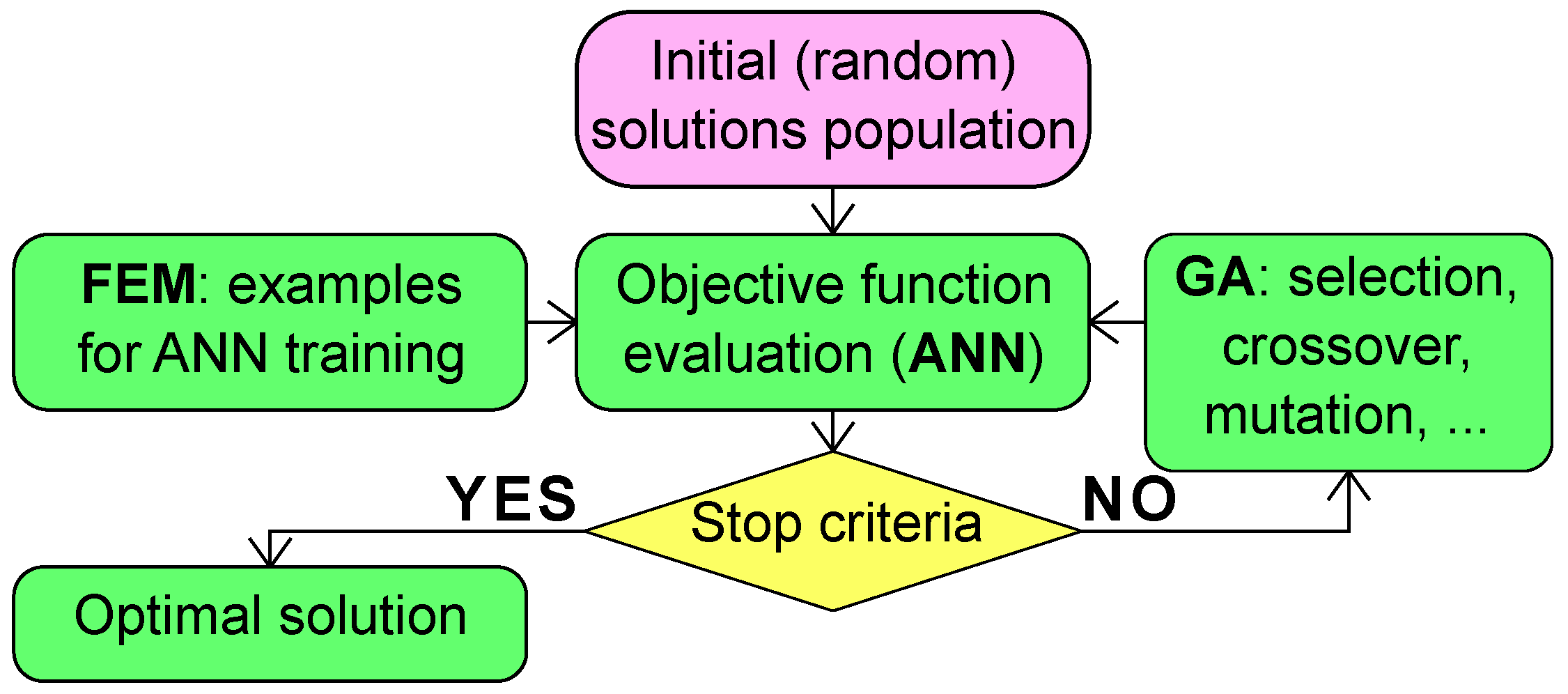
The scheme of the one-step optimization procedure proposed herein is shown in Figure 2 and is explained in the following:

• Initial solution population: Random generation of 100 vectors $\mathsf{\Lambda }\in {\mathbb{L}}^n$, where ${\lambda }^{min}=-90$ and ${\lambda }^{max}=+90$. In the jargon of GAs, each vector $\mathsf{\Lambda }$ is called a chromosome, and a set of $\mathsf{\Lambda }$ vectors is called a population. The dimension n of ${\mathbb{L}}^n$ space is determined by the number of lamination angles in $\mathsf{\Lambda }$.
• Objective function evaluation: For each chromosome ($\mathsf{\Lambda }$ vector of ${\lambda }_i$ lamination angles), the value of the objective function $\mathrm{g}\left(\mathsf{\Lambda }\right)$ being minimized (see Equations (7) and (8)) is calculated by a trained deep network: $g^{\mathrm{ANN}}(\mathsf{\Lambda })=\mathrm{ANN}(\mathsf{\Lambda })$.
• Stop criteria: All stop criteria are verified, e.g., the number of iterations is compared with the arbitrarily selected maximum, or the value of the decrease in the objective function in the subsequent iteration steps is compared with the required minimum.
• GA: selection, crossover, mutation: If the stop criteria are not fulfilled, the usual GA procedure involving selection, crossover, and mutation will produce a new population (a set of new $\mathsf{\Lambda }$ vectors), and the next iteration step begins.
• Optimal solution: When the stop criteria are fulfilled, the chromosome (${\mathsf{\Lambda }}^{\ast }$ vector) giving the smallest value of the objective function ${\mathsf{\Lambda }}^{\ast }=argmin\left\{\mathrm{g}(\mathsf{\Lambda })\right\}$ is treated as an optimal solution; the value of the objective function $\mathrm{g}\left({\mathsf{\Lambda }}^{\ast }\right)$ for the solutions obtained during multiple repetitions of the GA+ANN procedure with random initiation (denoted as ${\mathrm{g}}^{\mathrm{ANN}}\left({\mathsf{\Lambda }}^{\ast }\right)$ or ${\mathrm{g}}^{\mathrm{ANN}}$ for short) are verified by FEM (${\mathrm{g}}^{\mathrm{FEM}}\left({\mathsf{\Lambda }}^{\ast }\right)$ or ${\mathrm{g}}^{\mathrm{FEM}}$ for short). FEM is undoubtedly a more accurate method than ANN; therefore, as an optimal solution, the best ${\mathrm{g}}^{\mathrm{ANN}}$ resulting from multiple GA+ANN runs is not being chosen. Instead, the maximum value from among all obtained ${\mathrm{g}}^{\mathrm{FEM}}$ is chosen (the corresponding ANN prediction for the chosen ${\mathrm{g}}^{\mathrm{FEM}}$ is called ${\mathrm{g}}_{(\mathrm{ANN})}^{\mathrm{FEM}}$).

The procedure described above lacks one important step shown in Figure 2: the generation of patterns for ANN training and the training itself (in the figure, the step is labeled FEM: examples for ANN training). FE simulations obtain the patterns (or examples) that consist of already known values of the parameters to be obtained (i.e., the natural frequencies gathered in vector $\mathbf{f}$), together with varying parameters (lamination angles gathered in vector $\mathsf{\Lambda }$). This is the most time-consuming part of the whole procedure. In order to increase time efficiency in comparison with the procedure without ANN application, the number of FE calls during the generation of patterns for ANN training should be as low as possible; otherwise, this approach is pointless. The training of deep networks is relatively fast. In all analyzed cases, training took approximately 30 min on a 4-core system with Intel^® Core^® i5-4570 [email protected] GHz (Intel Corporation, Santa Clara, CA, USA) and 8 GB RAM and can be considered independent of the number of variables in the range considered herein.

3.2. Iterative Optimization (Curriculum Learning)

The one-step optimization procedure may be difficult to apply in a multi-dimensional space ${\mathbb{L}}^n$. Let us take the three-segment MODEL2 shell structure as an example (see Figure 1c). When each segment shell is composed of four symmetric layers of composite material (symmetric from the point of view of lamination angles), the overall number of different lamination angles reaches $n=6$. The generation of patterns with a dense ${\lambda }_i$ mesh may be, in this case, so time-consuming that even sophisticated approaches to the numerical experiment design are of no use.

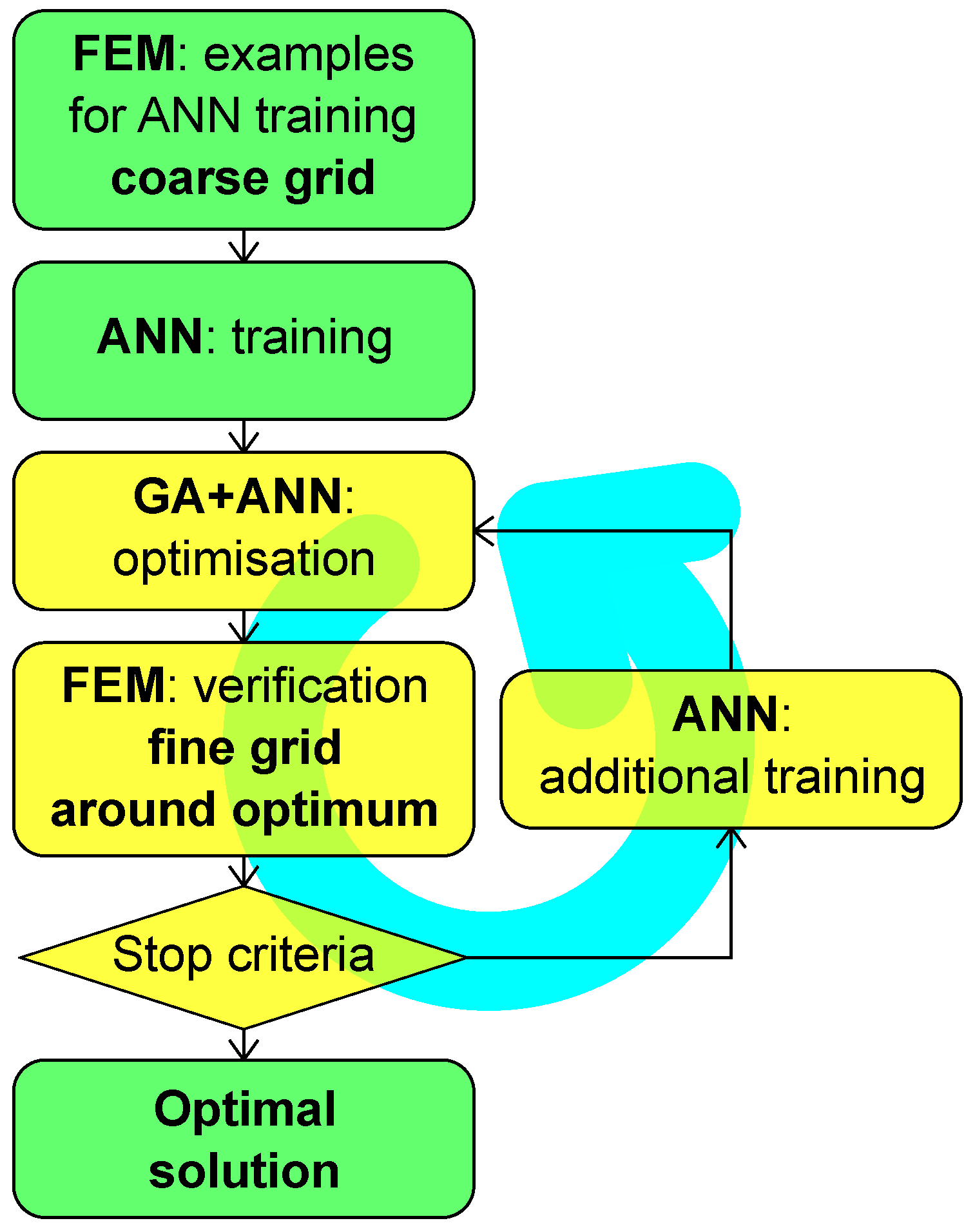
The novel idea of the optimization procedure to overcome the high-dimensionality problem described above is presented in Figure 3 and consists of the following steps:

• FEM examples for ANN training (coarse grid): ${\mathbb{L}}^n$ space is intentionally described by a limited number of patterns $\mathcal{P}={\{{(\mathbf{f},\mathsf{\Lambda })}^j\}}_{j=1}^P$. The role of the patterns is not to precisely describe the value of the objective function $\mathrm{g}(\mathsf{\Lambda })$ but to approximately locate the extremes of this function.
• ANN training: A deep network is trained to map $\mathsf{\Lambda }$ into $\mathbf{f}$; that is, the ANN should be capable of working as a function that returns vector ${\mathbf{f}}^j$ for a given vector ${\mathsf{\Lambda }}^j$: ${\mathbf{f}}^j=\mathrm{ANN}({\mathsf{\Lambda }}^j)$.
• GA+ANN optimization: GA optimization, with ANN applied to calculate the objective function, is performed; the result of this optimization is not significant with regard to a single ${\mathsf{\Lambda }}^{\ast }$ vector; the number of repetitions of this procedure should produce a set of ${\mathsf{\Lambda }}^{\ast ,k}$ vectors around the global minimum. Since there is a usual system shift of the results of GA+ANN optimization relative to the results of FEM (herein called “real” results), it would be advisable to interrupt GA optimization before it reaches any sharp minimum of ANN approximation of the objective function (possibly shifting from the “real” minimum of the objective function being sought).
• FEM verification (fine grid around the optimum): For each ${\mathsf{\Lambda }}^{\ast ,k}$ obtained in the previous step (there is not a single vector ${\mathsf{\Lambda }}^{\ast ,k}$ but a group of vectors since the tentative optimization in the previous step is repeated K times), a vector of natural frequencies ${\mathbf{f}}^{\ast ,k}$ is calculated ${\mathbf{f}}^{\ast ,k}=\mathrm{FEM}({\mathsf{\Lambda }}^{\ast ,k})$, and a new set of patterns is created ${\mathcal{P}}^{\ast }={\{{({\mathbf{f}}^{\ast },{\mathsf{\Lambda }}^{\ast })}^k\}}_{k=1}^K$.
• Stop criteria: The usual stop criteria are verified; if the criteria are not fulfilled, the procedure returns to GA+ANN optimization following additional ANN training (retraining).
• ANN additional training: The ANN already trained in the second step of the procedure is trained again (retrained) with the original set of patterns $\mathcal{P}$ expanded with ${\mathcal{P}}^{\ast }$; the ANN should then be more precise in the area of the expected global minimum.

The proposed procedure differs from the previously tested one (see Figure 2) in two major aspects: the pre-generation of a relatively small pattern set and the possibility of retraining the applied ANN with new patterns surrounding the optimum solution. The loop shown in Figure 3—application of GA+ANN optimization, generation of a fine grid of patterns around the optimum, and additional ANN training—is herein called Curriculum Learning (CL). The number following CL (e.g., CL2) shows the number of CL loops made (two in the case of CL2).

4. Verification Example

The optimization procedure described above, with GA as a tool to solve the optimization problem and ANN as a tool that substitutes time-consuming FE calculations, was verified using an example described in [41]. All of the following assumptions (regarding the FE model, material parameters, lamination angles, and so on) are based on this article.

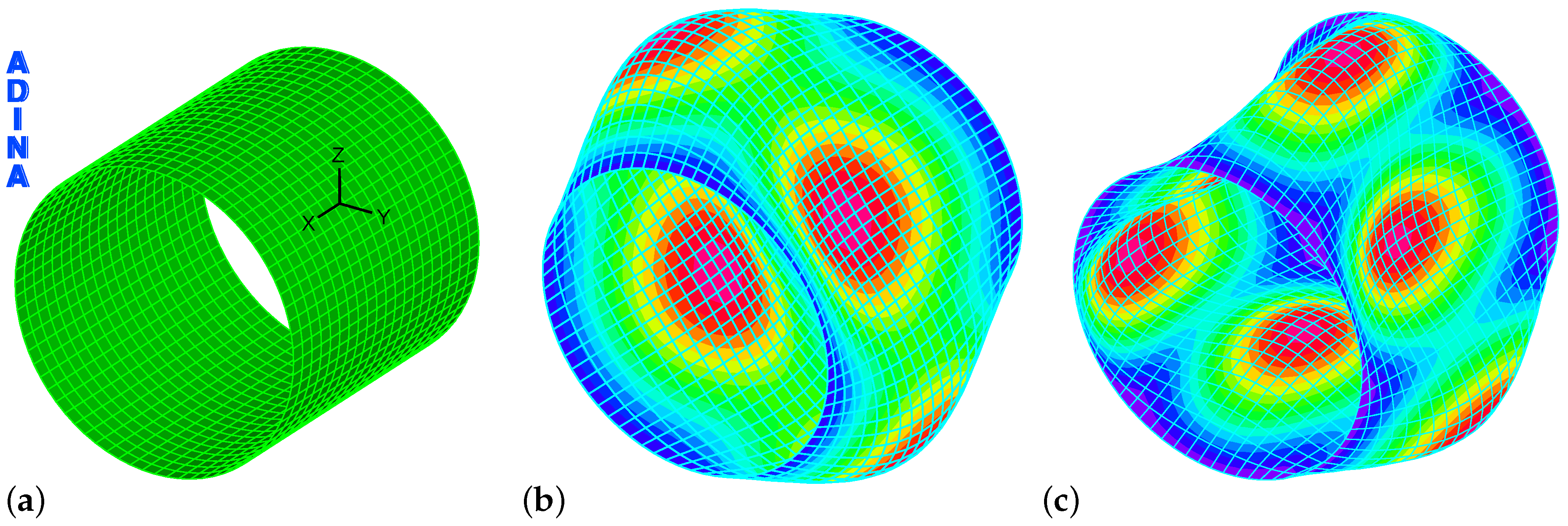
The structure (see Figure 4a) is a cantilever tube. Its model is a thin-walled cylindrical shell with a circular cross-section, and the diameter of the middle-surface of the cross-section is $R=0.1$ m. The thickness of the shell is $t=0.002$ m, and the length of the cantilever is $l=0.2$ m. The shell web consists of 64 layers of composite material of equal thickness but with different fiber orientations. The boundary conditions are defined on the cylinder axis and correspond to the support conditions of a simply supported beam. The material properties are $E_1=275.0$ GPa, $E_2=11.0$ GPa, ${\nu }_{12}=0.25$, $G_{12}=G_{13}=5.50$ GPa, and $\rho =1500$ kg/m${}^3$.

The lamination angles considered are 0, ±45, and 90. The laminates are considered symmetric, and neighboring layers are grouped into pairs, with lamination angles equal to $[0/0]$ (herein called ‘0’), $[+45/-45]$ (called ’$\pm 45$’), or $[90/90]$ (called ‘90’). For example, the stacking sequence described as ${[0_4/\pm {45}_8/{90}_4]}_s$ should be read as four pairs of layers $[0/0]$, eight pairs of layers $[+45/-45]$, and four pairs of layers $[90/90]$. Assuming that the stacking sequence is symmetric, the overall number of layers is equal to 64, while the number of varying lamination angles equals 16.

The fundamental natural frequency reported herein was obtained by using the commercial FE code ADINA [40]. The FE model (called MODEL3) was built using multi-layered shell 4-node MITC4 elements (first-order shear theory), the number of which equals 72 along the circumferential direction and 20 in the axial direction. The overall number of FE elements, nodes, and degrees of freedom equals 1440, 1514, and 9084, respectively.

In order to verify the compatibility of MODEL3 with the FE model used by Koide and Luersen in [41], the fundamental natural frequency was calculated for three different stacking sequences described in [41] and compared with the values in that paper. The results, shown in

Table 1. Fundamental frequency calculated by Koide and Luersen and by using MODEL3.

Stacking	${\mathit{f}}_1$ [Hz]	${\mathit{f}}_1$ [Hz]	Difference
Sequence	Koide and Luersen	MODEL3	[Hz]	[%]
${[0_{16}]}_s$	1803.4	1803.2	0.2	0.01
${[\pm {45}_{16}]}_s$	3450.3	3470.8	20.5	0.59
${[{90}_{16}]}_s$	2061.2	2062.4	1.2	0.06

, prove that the proposed FE model and the FE model in [41] can be considered compatible.

The optimization of the lamination angles in order to obtain the maximum value of the fundamental natural frequency $f_1$ was performed according to the scheme shown in Figure 2. Four pattern sets were generated. The first one, ${\mathcal{P}}_1$, consists of 5184 patterns, each composed of 16 angles of neighboring laminate pairs (ANN inputs) and one corresponding fundamental frequency (ANN output). The fundamental natural frequency corresponding to the particular set of lamination angles was computed using FEM. The patterns gathered in ${\mathcal{P}}_1$ were generated according to two scenarios:

• For the first three pairs of lamination angles, all three possible cases ($[0/0]$, $[+45/-45]$, and $[90/90]$) are considered. Starting from the fourth lamination angle pair to the 16th (the last one), two cases ($[0/0]$ and $[90/90]$) are considered for even lamination pairs (the 4th, the 6th, the 8th, and so on), and only one case ($[+45/-45]$) is considered for odd lamination angle pairs.
• For the first three pairs of lamination angles, all three possible cases ($[0/0]$, $[+45/-45]$, and $[90/90]$) are considered. Starting from the fourth lamination angle pairs to the 16th (the last one), one case ($[+45/-45]$) is considered for even lamination pairs, and two cases ($[0/0]$ and $[90/90]$) are considered for odd lamination angle pairs.

The second, the third, and the fourth pattern sets—${\mathcal{P}}_2$, ${\mathcal{P}}_3$, and ${\mathcal{P}}_4$—consist of 16 randomly generated angles of neighboring laminate pairs (ANN inputs) and one corresponding fundamental frequency (ANN output). The number of patterns in ${\mathcal{P}}_2$, ${\mathcal{P}}_3$, and ${\mathcal{P}}_4$ equal 1500, 3500, and 5000, respectively.

The pattern sets were applied in different combinations to train the deep network (see

Table 2. Comparison of optimized results.

	Pattern Sets in	${\mathit{f}}_1$ [Hz]	${\mathit{f}}_1$ [Hz]	${\mathsf{\Lambda }}^{\ast }$	No. of
	ANN Training	Koide and	MODEL3		FE
		Luersen [41]			Calls
Koide&Luersen	—	3529.4	3522.5	${[{90}_2/\pm {45}_{11}/0/90/\pm 45]}_s$	11,250
GA+ANN	${\mathcal{P}}_1+{\mathcal{P}}_4$	—	3581.4	${[90/\pm {45}_{13}/0_2]}_s$	10,234
GA+ANN	${\mathcal{P}}_2+{\mathcal{P}}_3+{\mathcal{P}}_4$	—	3581.4	${[90/\pm {45}_{13}/0_2]}_s$	10,050
GA+ANN	${\mathcal{P}}_1+{\mathcal{P}}_2$	—	3541.7	${[\pm {45}_5/90/\pm {45}_9/0]}_s$	6734
GA+ANN (CL1)	${\mathcal{P}}_1+{\mathcal{P}}_2$	—	3578.1	${[90/\pm {45}_{11}/0/\pm 45/0/\pm 45]}_s$	6784
GA+ANN	${\mathcal{P}}_2+{\mathcal{P}}_3$	—	3570.8	${[\pm {45}_{14}/0_2]}_s$	5050
GA+ANN (CL1)	${\mathcal{P}}_2+{\mathcal{P}}_3$	—	3581.4	${[90/\pm {45}_{13}/0_2]}_s$	5100
GA+ANN	${\mathcal{P}}_4$	—	3543.7	${[90/\pm 45/90/\pm {45}_3/0/\pm {45}_6/0/\pm {45}_2]}_s$	5050

ANN: artificial neural network; FE: finite element; GA: genetic algorithm.

), and the trained network substituted the FE simulations in the GA optimization of the lamination angles. The results reported herein from the GA+ANN optimization procedure, together with the results presented in [41], are shown in Table 2.

The results presented in Table 2 prove that the proposed GA+ANN optimization procedure is capable of solving the optimization problem. Moreover, even when applying a significantly smaller number of time-consuming FE calls, the results obtained by applying the GA+ANN procedure are still better than those presented in [41]. The proposed procedure is able to solve the optimization problem involving half the number of FE calls, which directly leads to considerable time-savings. Analysis of the results presented in Table 1 leads to the conclusion that there are multiple local maxima with $f_1$ equal to or higher than the value found in [41]. The value of $f_1=3581.4$ Hz seems to be a global extreme.

Special attention should be given to the results in the rows labeled “GA+ANN (CL1)”, which were obtained after one curriculum learning loop (see Figure 3). The CL approach was tested with all considered pattern set combinations and, in all of them, gave more precise ANN predictions of $f_1$ fundamental frequency. The cases shown in the rows “GA+ANN (CL1)” are those in which the CL approach also improved the optimization result. The most important observation is that the maximum of the fundamental frequency, which is higher than the one presented in [41], was obtained with half the number of FE calls (5100 instead of 11,250).

5. Optimization of the Three-Layer One-Segment Tube

5.1. Case Description

This rather simple problem was chosen to check the method’s accuracy and time consumption. Moreover, the use of three free model parameters makes the analysis of the behavior of the model’s natural frequencies possible. The investigated model, a six-meter-long laminate tube with three layers of composite material, is shown in Figure 1.

5.2. Classical FEM-Based Optimization Procedure

The average time necessary for FEM computations to find the first ten natural frequencies for a six-meter-long, three-layer non-symmetric laminate tube fixed at one end reaches approximately 13.9 s on a 4-core system with Intel^® Core^® i5-4570 [email protected] GHz and 8 GB RAM. This, of course, depends very much on the adopted FE mesh and the applied numerical procedure. However, it can be accepted as a basis for further consideration. The problem of maximization of the fundamental natural frequency $f_1$ needs the objective function, that is, $g(\mathsf{\Lambda })=-f_1(\mathsf{\Lambda })$, to be solved about 180 times on average. The parameters of the applied interior-point optimization algorithm (see [34,42]) are as follows: no constraints, no gradient nor Hessian supplied, maximum number of iterations equal to 100, 50 repetitions with a unique random starting point, and each calculation of the objective function needs an FE call. The exact number of objective function evaluations varies from 4 to 592, and the time necessary to perform $f_1$ maximization reaches an average of 25 min. However, for a particular case, it varies from 33 to 85 min (the time covers the entire optimization procedure, including all necessary FE simulations).

Each random initiation of the procedure leads to a different solution (and probably to a different local minimum). For 50 multi-start random initiations, the best-obtained result is $f_1=37.786$ Hz for lamination angles ${\mathsf{\Lambda }}^{\ast }=[50.9/-4.5/77.7]$. The overall time necessary to repeat the procedure 50 times and the number of FE calls are 21 h and 9061, respectively. The result of calculations involving classical, derivative-based optimization methods and FEM to obtain the objective function value is a reference point for the proposed GA+ANN optimization procedure. The genetic algorithm needs the objective function to be computed thousands of times, and for the maximization of $f_1$, the time necessary to obtain the results using FEM to calculate the objective function value would be 28 days. Obviously, this is an unacceptable time investment.

In order to make the GA procedure applicable with limited time constraints and typical computer hardware, the evaluation of natural frequencies was not done through FEM. Instead, neural networks were applied since, in contrast to FE simulations, a trained neural network is capable of giving its prediction almost instantly.

5.3. Pattern Generation and ANN Training

The procedure described above was tested on the MODEL1 structure (see Figure 1), with three layers of composite material and dense FE mesh applied during FEM computations. Patterns for ANN training were calculated using the FE ADINA code [40]. Each one is composed of three lamination angles $\mathsf{\Lambda }=\{{\lambda }_1,{\lambda }_2,{\lambda }_3\}$, one for each layer of the tube shell, and the corresponding natural frequencies of the tube $\mathbf{f}=\{f_1,f_2,\cdots ,f_{10}\}$:

$$\mathcal{P}={\{{(\mathbf{f},\mathsf{\Lambda })}^j\}}_{j=1}^P,$$

(11)

where the natural frequencies in pattern number j were obtained through FEM computations for lamination angles ${\mathsf{\Lambda }}^j$:

$${\mathbf{f}}^j=\{f_1^j,f_2^j,\cdots ,f_{10}^j\}=\mathrm{FEM}\left({\mathsf{\Lambda }}^j\right).$$

(12)

The number of natural frequencies computed amounted to ten in order to make the second optimization task (see Equation (8)) solvable. The patterns were generated on a regular grid in ${\mathbb{L}}^3$ space; that is, natural frequencies of the laminate tube were computed for all parameter vectors $\mathsf{\Lambda }=\{{\lambda }_1,{\lambda }_2,{\lambda }_3\}$, with ${\lambda }_i$ varying according to one of the scenarios gathered in

Table 3. Pattern sets.

Pattern				Number	Time Consumption
Set	${\mathit{\lambda }}^{min}$	${\mathit{\lambda }}^{max}$	$\mathbf{\Delta }\mathit{\lambda }$	of Patterns	Whole Set	One Pattern
${\mathcal{P}}_1$ (*)	−75	+75	30	216	53 min	14.6 s
${\mathcal{P}}_2$	−87	+88	35	216	51 min	14.0 s
${\mathcal{P}}_3$ (*)	−90	+90	30	343	82 min	14.3 s
${\mathcal{P}}_4$	−90	+90	15	2197	508 min	13.9 s
${\mathcal{P}}_5$	−90	+90	randomly	1000	243 min	14.6 s

(*) ${\mathcal{P}}_1$ and ${\mathcal{P}}_3$ are subsets of ${\mathcal{P}}_4$.

. Only the last pattern set ${\mathcal{P}}_5$ was generated with random values of lamination angles. The generation of patterns, together with ANN training, formed the longest part of the simulation (in Figure 2, it is labeled FEM: examples for ANN training), which predicts the actual optimization.

The penultimate column in Table 3 shows the duration of the generation of a particular ${\mathcal{P}}_i$ pattern set. The average time necessary to compute one pattern (the last column in Table 3) differs for particular sets since, in some cases, the method applied to solve the generalized eigenproblem (Equation (3)), namely, the subspace iteration method (see [30]), has to calculate a number of natural frequencies that is greater than the desired one (i.e., ten).

Pattern set generation is the most time-consuming part of the proposed GA+ANN procedure. The number of patterns should be large enough to accurately describe the function ${\mathbf{f}}^j=\mathrm{FEM}({\mathsf{\Lambda }}^j)$ and simultaneously small enough to ensure that the time necessary for their generation is acceptable. Obviously, the number of FE calls during pattern set generation should be significantly smaller than the number of FE calls during the classical minimization procedure (here that number is 9061) and the assumed number of FE calls during GA+FEM optimization (50 repetitions of GA optimization with 100 iterations of 100-element generation: 500,000 FE calls in total). In the considered case, the largest acceptable number of patterns was assumed to equal about 3000–4000. Some preliminary calculations showed that, instead of one pattern set generated using a regular grid (e.g., ${\lambda }^{min}=-90$, ${\lambda }^{max}=90$, $\Delta \lambda =12$), it is advisable to generate a few small pattern sets, each generated using a different grid and completed by a randomly generated pattern set. The considered pattern sets, described in Table 3, follow this preliminary conclusion. One of the goals of the following is to find a solution of a given optimization problem using the minimum number of patterns.

In the following experiment, five different learning sets were considered. In each case, the ANN was trained and tested on a different combination of ${\mathcal{P}}_i$ sets (see

Table 4. Deep network training and testing results.

Training	Testing	ANN	Training	Testing Error			No. of FE	Time
Pattern Sets	Pattern Sets	Symbol	Patterns	MSE	$\mathit{\sigma }$	ARE${}_1$	Calls	Consumption
${\mathcal{P}}_1+{\mathcal{P}}_3$	${\mathcal{P}}_2+{\mathcal{P}}_5$	ANN${}_{13}$	559	3.51	1.87	2.64	1775	459 min
${\mathcal{P}}_1+{\mathcal{P}}_2+{\mathcal{P}}_3$	${\mathcal{P}}_5$	ANN${}_{123}$	775	1.97	1.40	1.67	1775	459 min
${\mathcal{P}}_5$	${\mathcal{P}}_4$	ANN${}_5$	1000	3.42	1.85	2.69	3197	751 min
${\mathcal{P}}_1+{\mathcal{P}}_2+{\mathcal{P}}_3+{\mathcal{P}}_5$	${\mathcal{P}}_4-{\mathcal{P}}_1-{\mathcal{P}}_3$	ANN${}_{1235}$	1775	0.98	0.99	1.26	3413	802 min
${\mathcal{P}}_4$	${\mathcal{P}}_2+{\mathcal{P}}_5$	ANN${}_4$	2197	0.44	0.66	0.98	3413	802 min
${\mathcal{P}}_2+{\mathcal{P}}_4+{\mathcal{P}}_5$	none	ANN${}_{245}$	3413	—	—	—	3413	80 2min

ANN: artificial neural network; ARE: average relative error; FE: finite element; MSE: mean square error.

, the first column). In the last row of the table, the network ANN${}_{245}$ is described. All available patterns were used to train this network, so no testing was performed. The overall time consumption shown in the last column in Table 4 includes the time spent both on the generation of the learning and testing patterns as well as on network training.

The errors shown in Table 4 are commonly used error measures in ANN training, i.e., standard deviation $\sigma$, Mean Squared Error (MSE), and $f_1$ prediction Average Relative Error (ARE${}_1$). Assuming that $\mathbf{y}$ is the ANN prediction of natural frequencies,

$$\mathbf{y}=\{y_1,y_2,\cdots ,y_{10}\}=\mathrm{ANN}\left(\mathsf{\Lambda }\right).$$

(13)

MSE and ARE${}_1$ are given by the following formulas:

$$\mathrm{MSE}=\frac{1}{P}\sum _{j=1}^P\parallel {\mathbf{f}}^j-{\mathbf{y}}^j\parallel =\frac{1}{P}\sum _{j=1}^P\sum _{i=1}^{10}{(f_i^j-y_i^j)}^2,$$

(14)

$${\mathrm{ARE}}_1=\frac{1}{P}\sum _{j=1}^P\frac{f_1^j-y_1^j}{f_1^j}·100\%,$$

(15)

where P is the number of testing patterns (see Equation (10)).

The results shown in Table 4 prove that the applied deep networks are properly trained and can predict the values of the natural frequencies of a laminate tube with very high accuracy. However, the accuracy is significantly lower in two cases, namely, ANN${}_5$ (trained using random patterns only) and ANN${}_{13}$ (trained using a very limited number of patterns).

5.4. Maximization of the Fundamental Natural Frequency $f_1$

The maximization (optimization) of $f_1$ was performed by applying the procedure shown in Figure 2, with the following assumptions:

• the lamination angle increment is expressed either in real numbers (in the tables with the results coded as ‘0’), integer numbers (‘1’), or integers divisible by 2, 5, or 15 (‘2’, ‘5’, or ‘15’, respectively);
• the usefulness of all networks listed in Table 4 is verified;
• the GA optimization procedure for each lamination angle increment (‘0’, ‘1’, ‘2’, ‘5’, or ‘15’) and for each network (from ANN${}_{13}$ to ANN${}_{245}$) is repeated 50 times with different random initial populations.

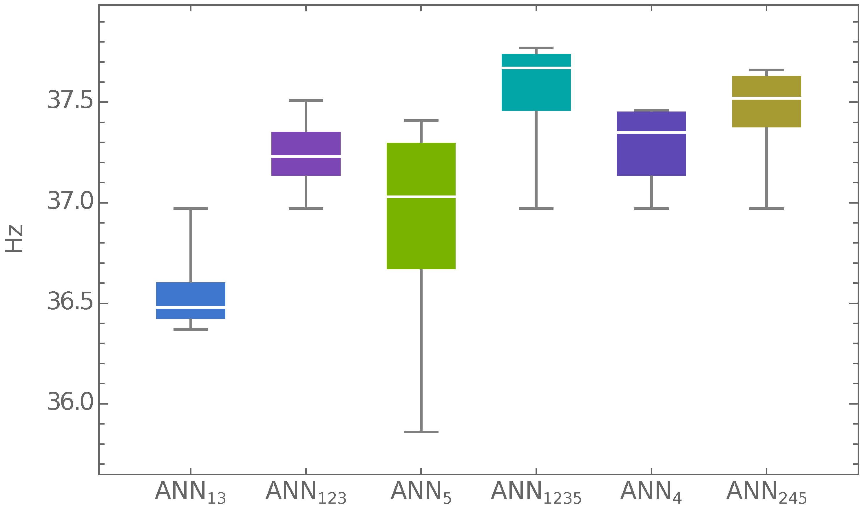
Altogether, the optimization procedure was repeated $5\times 6\times 50=1500$ times. The results obtained are illustrated in Figure 5.

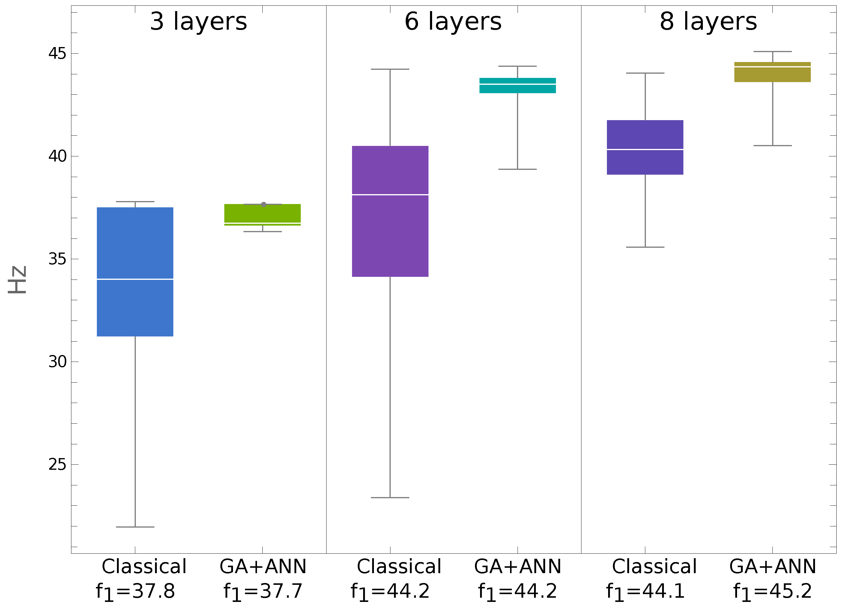
Figure 5 presents the so-called box-and-whisker diagram with the following metrics used to describe the results of 250 runs (five different lamination angle increments and 50 repetitions in each case) of $f_1$ maximization for a particular ANN applied: minimum and maximum values of the obtained results (whiskers); the interquartile range, representing the results between the 75th and 25th percentiles (the colored boxes); and the mean (the white lined inside the colored boxes). The box-and-whisker diagram was created using the $f_1^{max}={\mathrm{g}}^{FEM}$ results.

Of six verified networks, only one, ANN${}_{13}$, gave a mean result of $f_1^{max}={\mathrm{g}}^{FEM}$ that is lower than 36.97 Hz (the maximum value of $f_1$ available in the data sets). Four of the six networks gave a minimum of $f_1^{max}={\mathrm{g}}^{FEM}$ of almost 36.97 Hz, with the mean and the maximum clearly higher than 36.97 Hz. The best results are from applying optimization procedure using the ANN${}_{1235}$ network: the value $f_1=37.77$ Hz is almost 1 Hz higher than the value that can be found in rather dense sets of patterns.

The proposed optimization approach can be adopted for both real values of lamination angles and integer values with a user-defined angle increment. The rather narrow spread of results, e.g., those from ANN${}_4$, indicates the robustness of the proposed procedure. The time consumption of one optimization case (for example, using the network ANN${}_4$, a lamination angle increment of ‘0’, and 50 repetitions was one of the most time-consuming cases investigated) is 802 min for pattern generation, 15 s for GA+ANN optimization, and 22 min for FEM verification of the obtained results for a total time of slightly less than 14 h. The number of FE calls is 3413 during pattern generation and 50 during FE verification of GA+ANN results for a total of 3463 FE calls. For the network ANN${}_{1235}$, whose application generates the best-obtained results (for the increment ‘0’) of $f_1=37.67$ Hz and ${\mathsf{\Lambda }}^{\ast }=[51.5/-6.33/77.5]$, the overall time consumption is 9 min less, and the number of FE calls remains constant. In a reference case (classical optimization involving FEM), the best-obtained results are $f_1=37.786$ Hz and ${\mathsf{\Lambda }}^{\ast }=[50.9/-4.5/77.7]$, and the overall time and the number of FE calls are 21 h and 9061, respectively.

5.5. Maximization of the Distance between Natural Frequencies and a Selected Frequency

The main optimization task in the proposed approach is the maximization of the distance between an arbitrarily selected excitation frequency p and the neighboring natural frequencies (see Equation (8)). The considered values of p are 30, 40, 50, 60, 70, and 80 Hz.

The minimal difference between any natural frequency and any of the arbitrarily selected excitation frequencies is significantly higher than the targeted $10\%$ of the excitation frequency. Actually, in every case, it reaches $30\%$ of the excitation frequency p, whereas the minimum difference $|p-f_i|$ for every i should be higher than $10\%$ of p to avoid the resonance phenomenon.

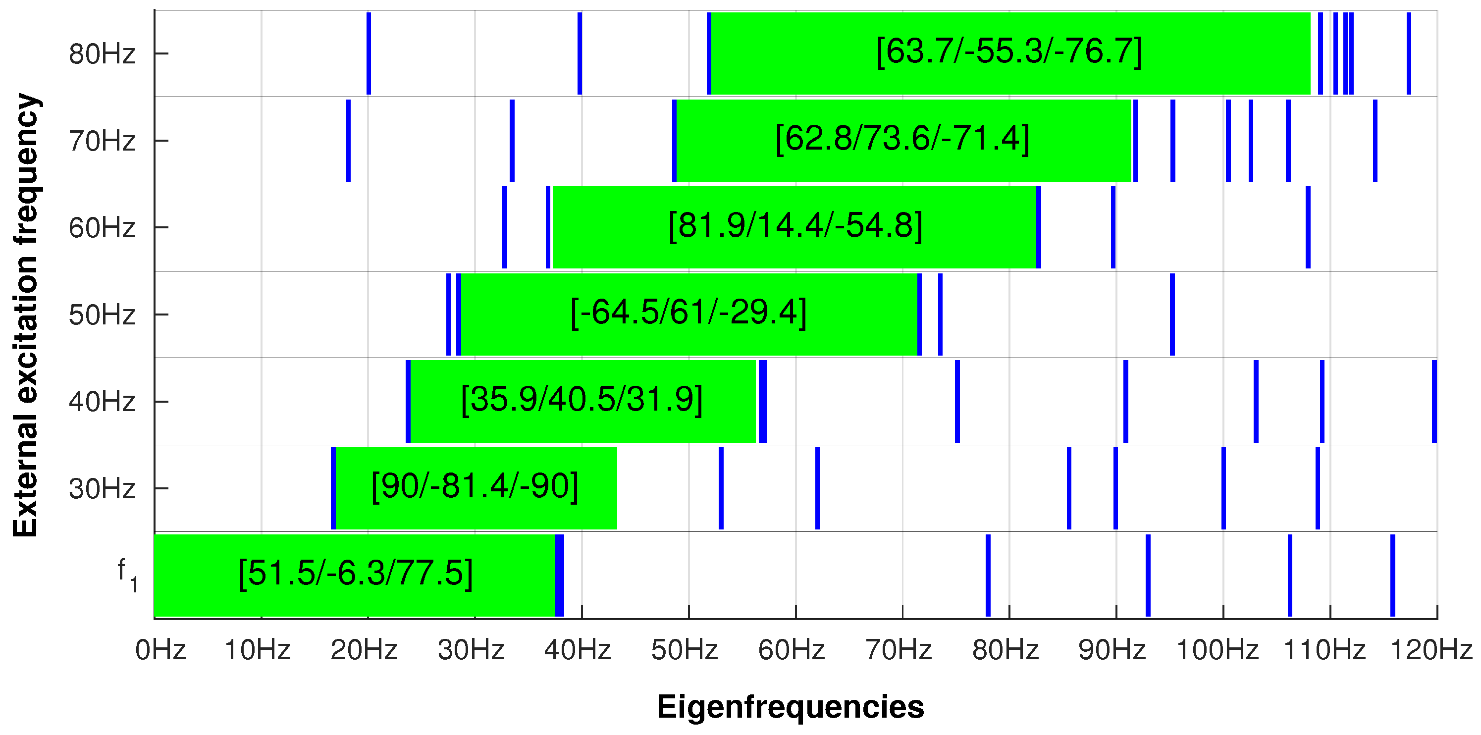
The results obtained from the ANN${}_{1235}$ network are presented in a graphical form in Figure 6. Successive rows in Figure 6 present the results of $f_1$ maximization (the bottom row) and the maximization of the distance between arbitrarily selected excitation frequencies (30–80 Hz) and natural frequencies calculated for MODEL1.

The green boxes represent the distance in the frequency space around a selected excitation frequency (30–80 Hz) that is free from natural frequencies and obtained when a particular set of lamination angles is applied. The blue vertical lines represent the natural frequencies calculated for the same lamination angles.

It is clearly visible that the ANN${}_{1235}$ network gives the expected results.

Table 5. Suggested lamination angles for different excitation force frequencies.

Excitation	Suggested	Minimal Distance
Frequency	Lamination	$|\mathit{p}-{\mathit{f}}_{\mathit{i}}|$
Range [Hz]	Angles	[Hz]	[%]
0.0–27.2	[51.5/−6.3/77.5]	10.5	38.5
27.2–38.4	[90/−81.4/−90]	14.6	38.2
38.4–42.6	[35.9/40.5/31.9]	14.1	33.2
42.6–54.2	[−64.5/61/−29.4]	17.4	32.1
54.2–65.7	[81.9/14.4/−54.8]	17.0	25.9
65.7–71.8	[62.8/73.6/−71.4]	20.0	27.8
>71.8	[63.7/−55.3/−76.7]	—	—

shows a kind of lookup table that enables the quick selection of lamination angles that lead to resonance avoidance for any excitation force frequency up to about 72 Hz. For example, for the excitation frequency $p=45$ Hz, the suggested lamination angle set [−64.5/61/−29.4] leads to a distance from $p=45$ Hz to the closest natural frequency $f_i$ of at least 17.4 Hz (or, expressed as a percentage, 32.1%). No calculations are necessary for resonance avoidance once Table 5 is ready.

Both problems, namely, the maximization of $f_1$ and the maximization of frequency gaps (eight optimization cases in total), were successfully solved using the ${\mathrm{ANN}}_{1235}$ network. The network ${\mathrm{ANN}}_{1235}$ was trained and tested using only 3413 FE calls during pattern set generation and 400 FE calls during the verification of obtained results. If it is assumed that the number of FE calls necessary to perform the same tasks using the classical optimization approach exceeds 70,000 (eight optimization cases, each needing about 9000 FE calls), then, in the GA+FEM approach, the number of FE calls reaches 4,000,000. The number of FE calls in the application of the proposed GA+ANN procedures decreases by at least one order of magnitude compared with the classical optimization approach.

6. Optimization of MODEL1 Structure with a Different Number of Layers

The optimization of the fundamental natural frequency $f_1$ and the distance between an arbitrarily selected excitation frequency p and the neighboring natural frequencies was performed with the number of layers equaling 2, 3, 4, 6, and 8. In three cases, including the one described above, the classical FEM-based optimization procedure was also applied to verify the results obtained from the GA+ANN procedure (see

Table 6. Results of $f_1$ optimization using classical and proposed procedures using MODEL1 with a different number of layers.

Optimization	Best	Optimal	No. of FE
Approach	Result [Hz]	Angles	Calls
3 layers
Classical	37.8	[50.9/−4.5/77.7]	9061
GA+ANN	37.7	[51.5/−6.3/77.5]	3463
6 layers
Classical	44.2	[70.0/8.5/−4.6/−30.6/9.4/85.1]	17,255
GA+ANN	44.2	[73.7/−13.3/−10.7/16.1/10.8/−89.9]	9971
8 layers
Classical	44.1	[−77.7/5.9/59.3/−4.6/−3.3/29.8/−18.5/87.8]	22,652
GA+ANN	45.2	[78.7/−46/5.94/4.64/5.43/−0.637/−3.15/89.9]	12,714

ANN: artificial neural network; GA: genetic algorithm.

and Figure 7 for details). The results obtained from the GA+ANN procedure are at least as accurate as the ones obtained from the classical FEM-based procedure (for the more complicated examples, they are even slightly better), though the number of FE calls is significantly smaller.

Table 7. Numerical results of $f_1$ optimization using MODEL1 with a different number of layers.

Fiber	Optimal	Optimal Solution [Hz]
Angle	Lamination	${\mathit{f}}_1^{max}$	${\mathit{f}}_1^{max}$
Increment	Angles ${\mathsf{\Lambda }}^{\ast }$	${\mathbf{g}}_{(\mathbf{FEM})}^{\mathbf{ANN}}$	${\mathbf{g}}^{\mathbf{FEM}}$
3 layers
0	[51.5/−6.33/77.5]	37.33	37.67
1	[51/−6/77]	37.32	37.73
5	[−55/5/−75]	37.27	37.77
6 layers
0	[73.7/−13.3/−10.7/16.1/10.8/−89.9]	43.88	44.17
1	[75/5/−17/8/6/−90]	44.02	43.76
5	[−70/−5/20/−5/0/−90]	43.79	43.79
8 layers
0	[78.7/−46/5.94/4.64/5.43/−0.637/−3.15/89.9]	44.94	45.24
1	[82/−37/16/−2/6/−2/−7/90]	45.01	44.99
5	[85/−35/20/0/5/−5/−5/90]	44.95	45.08

and

Table 8. Optimization of the distance between natural frequencies and $p=70$ Hz using MODEL1 with a different number of layers.

Fiber	Optimal	Optimal Solution [Hz]
Angle	Lamination	$min|{\mathit{f}}_{\mathit{i}}({\mathsf{\Lambda }}^{\ast })-\mathit{p}|$
Increment	Angles ${\mathsf{\Lambda }}^{\ast }$	${\mathbf{g}}_{(\mathbf{FEM})}^{\mathbf{ANN}}$	${\mathbf{g}}^{\mathbf{FEM}}$
3 layers
0	[62.8/73.6/−71.4]	21.62	21.36
1	[66/81/−69]	21.91	21.09
5	[−55/−70/85]	22.11	20.72
6 layers
0	[76.4/−22.9/7.82/17.6/16.8/−60.9]	23.75	23.44
1	[90/−11/−13/23/26/−61]	25.19	23.20
5	[−70/−10/20/−5/0/−90]	23.80	20.36
8 layers
0	[70.6/−43.3/13.9/−3.89/−2.19/−13.7/18.8/72.5]	24.35	24.32
1	[72/−46/21/9/−3/−5/−16/70]	24.54	24.55
5	[75/−40/25/0/5/−5/−20/70]	24.67	24.39

present the results of the optimization of the MODEL1 structure.

The results of $f_1$ maximization show the stabilization of the fundamental natural frequency value; further increasing the number of layers does not result in an associated increase in $f_1$. The same conclusion can be drawn when maximizing the distance between natural frequencies and a selected excitation frequency.

7. Optimization of the Four-Layer Three-Segment Tube

7.1. Pattern Generation and ANN Training

The proposed CL optimization improvement (see Figure 3) was tested on the MODEL2 structure (see Figure 1c), with four symmetric layers of composite material and sparse FE mesh applied during FEM computations. The number of different lamination angles equals six, i.e., $\mathsf{\Lambda }=[{\lambda }_1/{\lambda }_2|{\lambda }_3/{\lambda }_4{|{\lambda }_5/{\lambda }_6]}_s\in {\mathbb{L}}^6$. The lamination angles in the first segment (the one with the highest diameter) are ${[{\lambda }_1/{\lambda }_2]}_s=[{\lambda }_1/{\lambda }_2/{\lambda }_2/{\lambda }_1]$; the angles in the second one (the one with non-constant diameter) are ${[{\lambda }_3/{\lambda }_4]}_s=[{\lambda }_3/{\lambda }_4/{\lambda }_4/{\lambda }_3]$; and the angles in the last one are ${[{\lambda }_5/{\lambda }_6]}_s=[{\lambda }_5/{\lambda }_6/{\lambda }_6/{\lambda }_5]$.

Two groups of pattern sets for ANN training were calculated using the FE ADINA code [40]. Each was composed of lamination angles $\mathsf{\Lambda }=[{\lambda }_1/{\lambda }_2|{\lambda }_3/{\lambda }_4{|{\lambda }_5/{\lambda }_6]}_s$ and the corresponding fundamental frequency of the structure $\mathbf{f}=\{f_1\}$ or ten corresponding natural frequencies of the structure $\mathbf{f}=\{f_1,f_2,\cdots ,f_{10}\}$:

$$\mathcal{P}={\{{(\mathbf{f},\mathsf{\Lambda })}^p\}}_{p=1}^P,$$

(16)

where the fundamental frequencies were obtained through FEM computations. The details concerning pattern generation are summarized in

Table 9. Pattern sets (three-segment MODEL2).

Pattern				Number	Time Consumption
Set	${\mathit{\lambda }}^{min}$	${\mathit{\lambda }}^{max}$	$\mathbf{\Delta }\mathit{\lambda }$	of Patterns	${\mathit{f}}_1$	${\mathit{f}}_1$ through ${\mathit{f}}_{10}$
Training sets
${\mathcal{P}}_1$	−60	+60	60	729	44 min	97 min
${\mathcal{P}}_2$	−75	+75	60/30/60 (*)	4096	248 min	546 min
${\mathcal{P}}_3$	−90	+90	60	4096	248 min	546 min
${\mathcal{P}}_4$ (**)	−90	+90	randomly	1000	61 min	133 min
Testing sets
${\mathcal{P}}_5$	−75	+75	30	4000 (***)	243 min	533 min
${\mathcal{P}}_6$	−87	+88	35	4000 (***)	243 min	533 min

(*) $\Delta \lambda$ was not constant, and the considered values are ${\lambda }_i=(-75,-15,+15,+75)$; (**) ${\mathcal{P}}_4$ is not used in $f_1$ maximization; (***) only 4000 randomly selected patterns out of 46,656 patterns were generated.

. The length of time required to generate one pattern is shorter than that in the previous case of MODEL1 optimization since the sparse FE mesh was applied (the number of finite elements is four times smaller than that in the case of the dense FE mesh).

The minimum and maximum values of the first ten natural frequencies (in [Hz]) that could be found in the pattern sets are $f_1\in (50.25,90.31)$, $f_2\in (54.31,95.91)$, $f_3\in (67.97,109.47)$, $f_4\in (74.77,116.65)$, $f_5\in (91.03,151.66)$, $f_6\in (92.87,152.67)$, $f_7\in (110.16,169.93)$, $f_8\in (110.41,175.39)$, $f_9\in (121.12,179.44)$, and $f_{10}\in (128.03,212.70)$.

Two deep networks were trained for $f_1$ maximization, and the difference between them is the number of learning patterns: ANN${}_3^1$ was trained with 4096 patterns, while ANN${}_{123}^1$ was trained with 8,921 patterns. Another two, ANN${}_{123}^{10}$ and ANN${}_{1234}^{10}$, were trained for the maximization of the distance between natural frequencies and a selected frequency.

7.2. Maximization of the Fundamental Natural Frequency $f_1$

The maximization (optimization) of $f_1$ was performed by applying the procedure shown in Figure 3, with the following assumptions:

• the lamination angle increment is expressed only in real numbers, and other approaches are not tested,
• the usefulness of the two networks (ANN${}_3^1$ and ANN${}_{123}^1$, see

  Table 10. Deep network training and testing results (three-segment MODEL2).

  Training	Testing	ANN	Training	Testing Error			No. of FE	Time
  Pattern Sets	Pattern Sets	Symbol	Patterns	MSE	$\mathit{\sigma }$	ARE${}_1$	Calls	Consumption
  one-output networks ($f_1$ only)
  ${\mathcal{P}}_3$	${\mathcal{P}}_5+{\mathcal{P}}_6$	ANN${}_3^1$	4,096	10.45	3.23	3.53	12,096	736 min
  ${\mathcal{P}}_1+{\mathcal{P}}_2+{\mathcal{P}}_3$	${\mathcal{P}}_5+{\mathcal{P}}_6$	ANN${}_{123}^1$	8,921	3.69	1.92	1.91	16,921	1,017 min
  ten-output networks (from $f_1$ to $f_{10}$)
  ${\mathcal{P}}_1+{\mathcal{P}}_2+{\mathcal{P}}_3$	${\mathcal{P}}_4$	ANN${}_{123}^{10}$	8921	12.28	3.50	2.26	9921	1353 min
  ${\mathcal{P}}_1+{\mathcal{P}}_2+{\mathcal{P}}_3+{\mathcal{P}}_4$	none	ANN${}_{1234}^{10}$	9921	—	—	—	9921	1353 min

  ANN: artificial neural network; ARE: average relative error; FE: finite element; MSE: mean square error.

  ) is verified,
• different numbers of generations of GA optimization are applied to prevent GA from achieving a sharp minimum during intermediate optimization loops,
• the GA optimization procedure for each network and each considered number of generations is repeated 50 times, with different random initial populations.

Altogether, the optimization procedure was repeated $19\times 50=950$ times. The results obtained are shown in Figure 8 and

Table 11. Numerical results of $f_1$ optimization using MODEL2 with four symmetric layers of laminate.

ANN	CL	Optimal Lamination Angles	Optimal Solution [Hz]
Type	Level	${\mathsf{\Lambda }}^{\ast }$	${\mathbf{g}}_{(\mathbf{FEM})}^{\mathbf{ANN}}$	${\mathbf{g}}^{\mathbf{FEM}}$
	CL0	[−69.5/6.07|89.9/−12.7|−82.9/−7.08]	90.47	94.06
ANN${}_3^1$	CL1	[−63.3/14.6|89.7/−9.61|88.1/−9.58]	93.03	94.24
	CL2	[−57.4/10.2|89.8/−4.18|89.8/5.35]	94.97	95.43

ANN: artificial neural network; CL: curriculum learning.

.

The total number of GA generations (see Table 11, the third column) was not only $G=100$ (as it was for every case of MODEL1 optimization) but also $G=50$ and $G=75$. The number of generations was increased to $G=200$ in only one case (the last row of Table 11) in order to check whether such an extension of the procedure would be expedient. Since there are no observable improvements with this increase, $G=100$ is treated as the appropriate value.

Figure 8 shows a clear improvement in the results, especially for ANN${}_3^1$, which was trained on the data set ${\mathcal{P}}_3$, which is half the size of the training set ${\mathcal{P}}_1+{\mathcal{P}}_2+{\mathcal{P}}_3$ used for the second network, ANN${}_{123}^1$. The final results obtained from both networks are comparable. However, the time required to generate the necessary pattern set, train the networks, and perform the optimization procedure is significantly different: 792 min (13.2 h) for ANN${}_3^1$ and 1073 min (17.9 h) for ANN${}_{123}^1$.

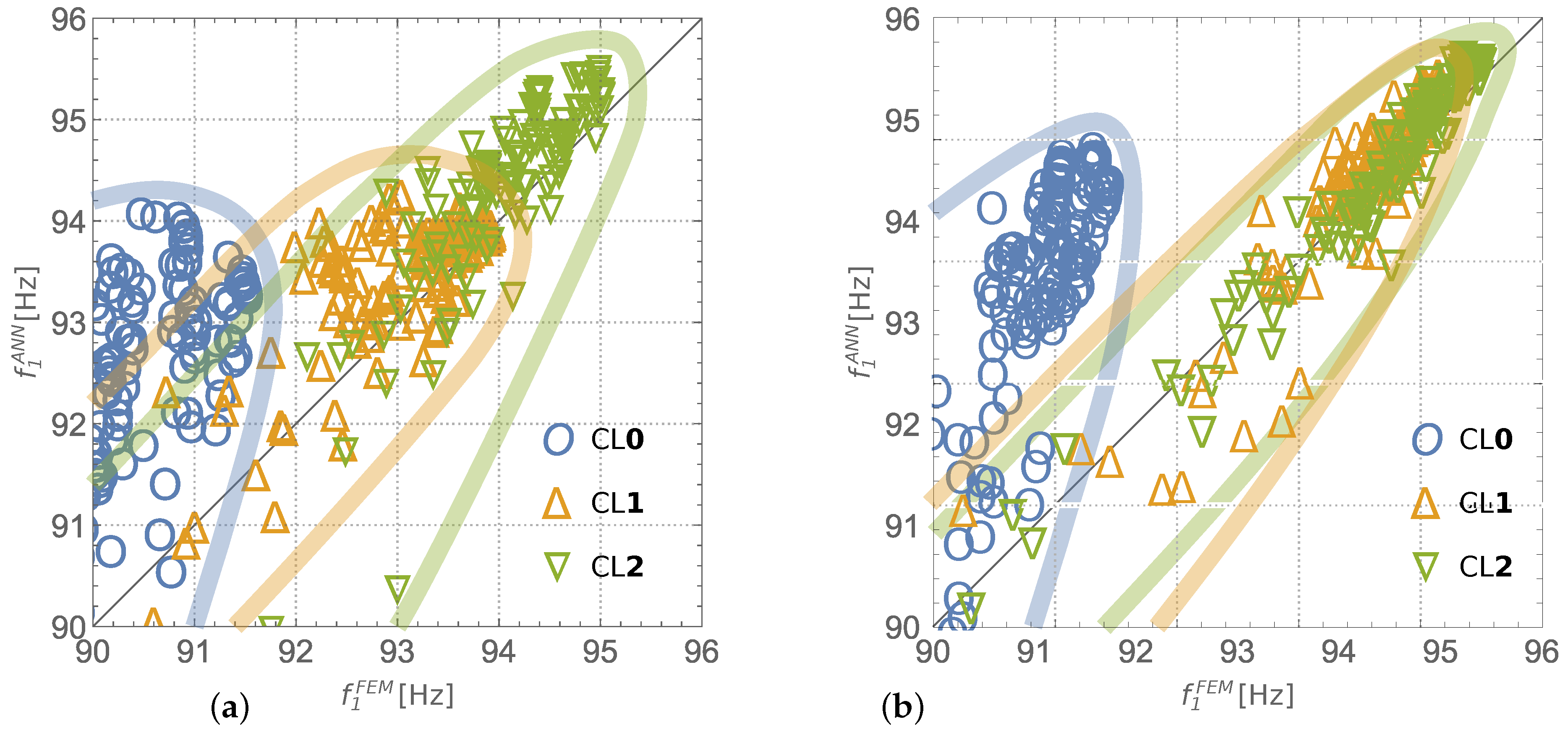
The mechanism of improvement during three CL loops in the application of ANN${}_3^1$ is clearly visible in Figure 9. The results obtained from ANN${}_3^1$ and ANN${}_{123}^1$ are visualized in a manner that is typical for the presentation of neural network accuracy: $f_1^{\mathrm{ANN}}$ versus $f_1^{\mathrm{FEM}}$ (values predicted versus desired). Obviously, the better the network training, the closer the points—i.e., the networks’ results—to the diagonal $y=x$ line. There are three types of points in the figure: circles represent the results of the pretrained network (trained using the initially generated pattern set ${\mathcal{P}}_3$), triangles represent the results of the networks retrained using additional patterns obtained after the first CL loop, and, finally, the upside-down triangles represent the results of the networks retrained again using additional patterns obtained after the second CL loop.

Larger values on the horizontal axis in the subsequent steps of the optimization algorithm (CL0, CL1, and CL2) are indicative of additional patterns gathered after successive loops approaching the desired extreme. The decreasing distances from the diagonal $y=x$ line mean that the retrained networks acquire a higher level of accuracy around the global extreme. Figure 9a presents a visible improvement in ANN${}_3^1$ after each of the CL loops, and the ANN${}_{123}^1$ network (see Figure 9b) clearly improves after the CL1 loop. The next loop CL2 does not significantly improve the maximum $f_1$ value, but it increases the network accuracy for the lower values of $f_1$.

7.3. Maximization of the Distance between Natural Frequencies and a Selected Frequency

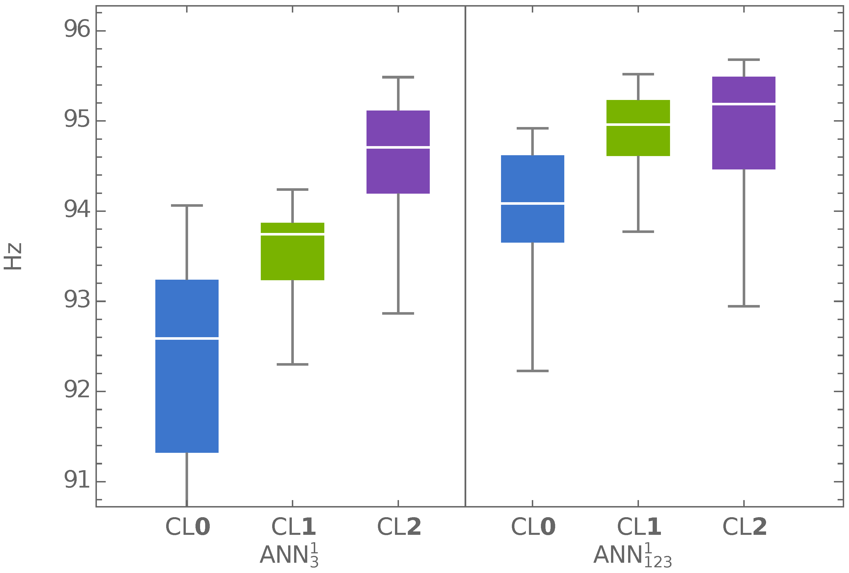
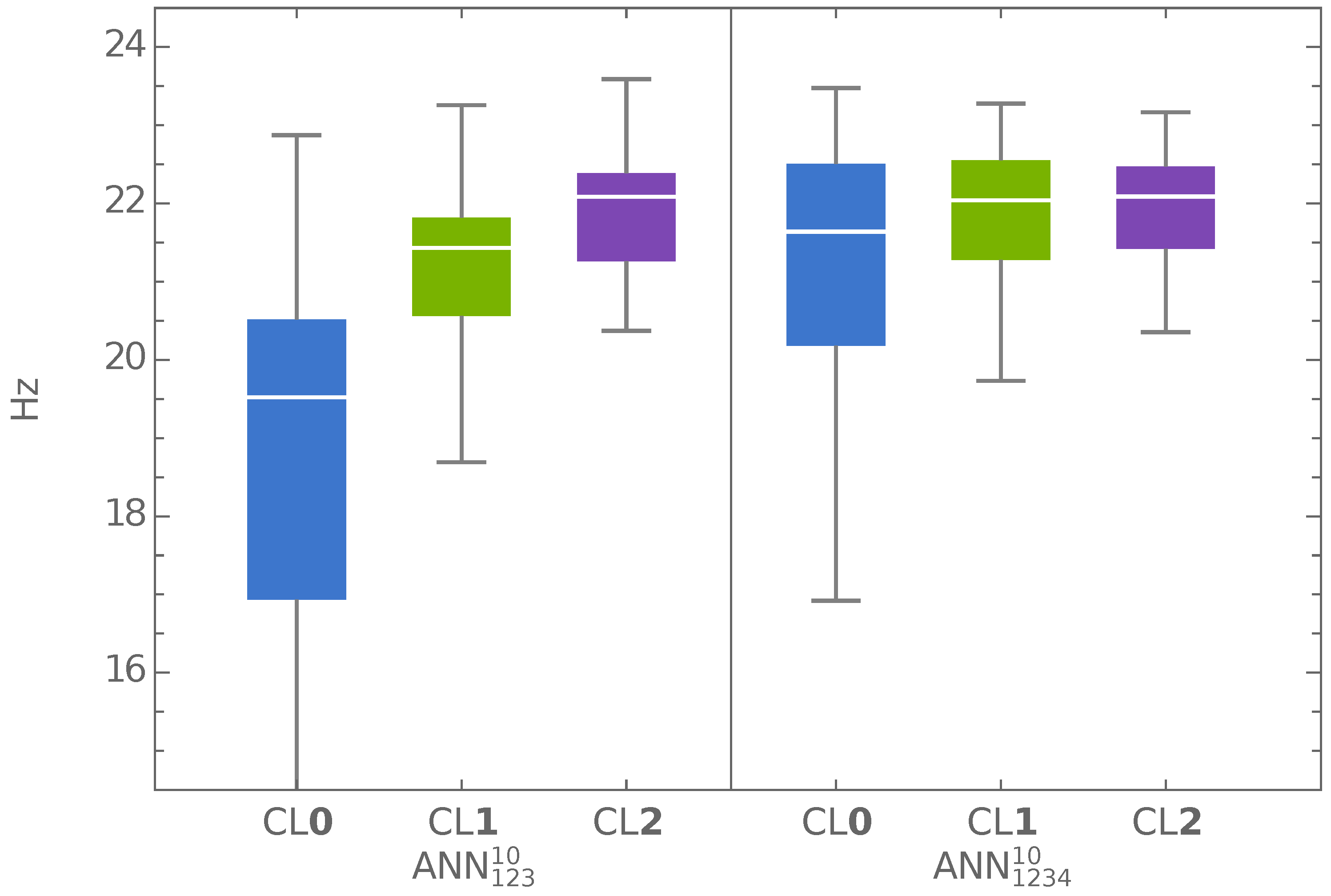
The last example discussed in detail is the maximization of the distance between natural frequencies and an arbitrarily selected excitation frequency (see Equation (8)). The considered external excitation frequencies are $p=90$, $p=100$, $p=110$, $p=120$, and $p=130$ Hz. These values of p are assumed to be within the frequency variation limits, which range from $f_1$ to $f_{10}$. Figure 10 shows the results (as a box-and-whisker diagram) of three optimization loops in the application of either ANN${}_{123}^{10}$ or ANN${}_{1234}^{10}$ for an external excitation frequency of $p=120$ Hz.

The improvement is clearly visible, especially for the first network. The ANN${}_{123}^{10}$ network, which was trained on a data set that was smaller than the one used to train ANN${}_{1234}^{10}$, finally yields equally precise results after three CL loops.

The results for the maximization of the distance between natural frequencies and the considered excitation frequencies are presented in

Table 12. Optimization of the distance between natural frequencies and selected excitation frequencies using MODEL2 with four symmetric layers of laminate.

ANN	CL	Optimal Lamination Angles	Optimal Solution [Hz]
Type	Level	${\mathsf{\Lambda }}^{\ast }$	${\mathbf{g}}_{(\mathbf{FEM})}^{\mathbf{ANN}}$	${\mathbf{g}}^{\mathbf{FEM}}$
Excitation frequency $p=90$ Hz
	CL0	[−76/16.7|-30/13.3|30.2/−36.5]	20.50	21.87
ANN${}_{1234}^{10}$	CL1	[−74.5/15.4|−31.1/12.9|29.8/−36.4]	21.73	22.24
	CL2	[76/−15.1|−27.7/10.5|31.5/−32.2]	21.93	22.03
Excitation frequency $p=100$ Hz
	CL0	[−75.1/−45.7|49/53.1|83.7/89.9]	21.30	20.91
ANN${}_{1234}^{10}$	CL1	[−62.1/−35.2|56.3/64.2|86.1/90]	21.58	21.61
	CL2	[−69.2/−39.9|52.9/52.3|87.8/89.9]	22.08	22.06
Excitation frequency $p=110$ Hz
	CL0	[−84.4/−16.3|59.2/29.2|-84.7/−88]	23.48	23.26
ANN${}_{1234}^{10}$	CL1	[90/−18.1|-56.8/-33.4|89.5/89.9]	23.39	23.41
	CL2	[−80.4/−16.3|61.2/31.3|−88.7/89.9]	23.58	23.60
Excitation frequency $p=120$ Hz
	CL0	[−89.8/−16.9|67.5/0.925|86.8/−63.2]	24.04	23.48
ANN${}_{1234}^{10}$	CL1	[87.9/−12.4|78.5/0.972|−79.7/−59.4]	23.97	23.28
	CL2	[−86.2/−19.7|72.4/27.6|90/−9.59]	22.89	23.17
Excitation frequency $p=130$ Hz
	CL0	[85/−13.6|75/0.252|90/11.1]	21.64	22.56
ANN${}_{1234}^{10}$	CL1	[82/−12.4|−84.5/0.366|−74.8/11.1]	22.14	22.28
	CL2	[77.2/−15|80.6/1.29|90/14.5]	22.64	23.31

ANN: artificial neural network; CL: curriculum learning.

. The minimum difference between any natural frequency and any of the arbitrarily selected excitation frequencies is significantly higher than the desired $10\%$ of the excitation frequency (as in the case for the MODEL1 structure). In every case, the difference is almost $20\%$ of the excitation frequency p.

8. Conclusions

This paper presents a novel method for the optimization of the stacking sequence in laminated structures. The proposed method is robust and efficient in simple optimization cases as well as in more complicated problems with more design variables. Complex boundary conditions, the complicated shape of the investigated structures, and the type of variable (continuous or discrete) do not hinder the effective use of the method. Moreover, the procedure can be successfully applied to optimization cases in which it is not possible to derive analytical formulae that combine design variables and optimized quantities.

As a result of replacing the finite element method by deep neural networks for the calculation of the optimized structure parameters, the proposed method significantly accelerates the optimization and enables the optimization to be performed in limited time on typical computer hardware. In addition to instantly calculating the objective function, deep neural networks have another important advantage: they facilitate the use of a very large number of patterns describing the optimization space. In the examples described in this paper, the number of available patterns reaches $10,000$. In other cases, which are not discussed in this paper, deep networks were trained on $120,000$ patterns, and the training time did not exceed 30 min.

The main idea presented in this paper, i.e., the curriculum learning of the applied deep networks, opens the door to new applications of the combined GA+ANN optimization procedure. The procedure can start with a very sparse description of the optimization space, and, in the successive iteration steps, the space description acquires a higher level of accuracy around the global minimum. The increasing accuracy of the objective space description and the possibility of deep network retraining presents the opportunity to create a very precise neural approximation of optimized structure parameters and, therefore, to significantly increase the precision of GA+ANN optimization.

The combined GA+ANN procedure was successfully applied to problems related to the avoidance of vibration resonance, which is a major concern for every structure subjected to periodic external excitations. The presented examples show two approaches to resonance avoidance: the maximization of the fundamental natural frequency (for external excitation frequencies possibly smaller than the fundamental natural frequency) or the maximization of a frequency gap around the external excitation frequencies (in other cases). In all examples presented in this paper, the necessary changes in natural frequencies are the result of appropriate changes in lamination angles only. In other words, no changes in the boundary conditions, geometry, or mass of the structures are introduced.

A further study of the proposed optimization procedure would be of interest. The proposed problems to be discussed include the following:

• vibration resonance avoidance in the case of a few periodic excitations with different frequencies;
• multi-criteria optimization, e.g., the maximization of the fundamental natural frequency, together with the maximization of the buckling force;
• composite material design (e.g., topological constraints, varying thickness and/or stiffness);
• a full variable–stiffness approach to lamination parameters that considers continuous changes in lamination parameters over the investigated domain;
• multi-dimensional problems with the number of design variables exceeding twenty; and
• optimization of a shell with openings.

References

1. Reddy, J. Mechanics of Laminated Composite Plates and Shells: Theory and Analysis; CRC Press: Boca Raton, FL, USA, 2004. [Google Scholar]
2. Nikbakt, S.; Kamarian, S.; Shakeri, M. A review on optimization of composite structures Part I: Laminated composites. Compos. Struct. 2018, 195, 158–185. [Google Scholar] [CrossRef]
3. Siwowski, T.; Kaleta, D.; Rajchel, M. Structural behaviour of an all-composite road bridge. Compos. Struct. 2018, 192, 555–567. [Google Scholar] [CrossRef]
4. Markiewicz, B.; Ziemiański, L. Numerical modal analysis of the FRP composite beam. J. Civ. Eng. Environ. Archit. 2015, 62, 281–293. [Google Scholar] [CrossRef]
5. Nayfeh, A.; Pai, P. Linear and Nonlinear Structural Mechanics; Wiley Series in Nonlinear Science; Wiley: New York, NY, USA, 2008. [Google Scholar]
6. Qatu, M.S.; Sullivan, R.W.; Wang, W. Recent research advances on the dynamic analysis of composite shells: 2000–2009. Compos. Struct. 2010, 93, 14–31. [Google Scholar] [CrossRef]
7. Ghiasi, H.; Pasini, D.; Lessard, L. Optimum stacking sequence design of composite materials Part I: Constant stiffness design. Compos. Struct. 2009, 90, 1–11. [Google Scholar] [CrossRef]
8. Ghashochi Bargh, H.; Sadr, M.H. Stacking sequence optimization of composite plates for maximum fundamental frequency using particle swarm optimization algorithm. Meccanica 2012, 47, 719–730. [Google Scholar] [CrossRef]
9. Vo-Duy, T.; Ho-Huu, V.; Do-Thi, T.; Dang-Trung, H.; Nguyen-Thoi, T. A global numerical approach for lightweight design optimization of laminated composite plates subjected to frequency constraints. Compos. Struct. 2017, 159, 646–655. [Google Scholar] [CrossRef]
10. Setoodeh, S.; Abdalla, M.M.; Gürdal, Z. Design of variable–stiffness laminates using lamination parameters. Compos. Part B Eng. 2006, 37, 301–309. [Google Scholar] [CrossRef]
11. Abouhamze, M.; Shakeri, M. Multi-objective stacking sequence optimization of laminated cylindrical panels using a genetic algorithm and neural networks. Compos. Struct. 2007, 81, 253–263. [Google Scholar] [CrossRef]
12. Waszczyszyn, Z.; Ziemiański, L. Neural Networks in Mechanics of Structures and Materials-New Results and Prospects of Applications. Comput. Struct. 2001, 79, 2261–2276. [Google Scholar] [CrossRef]
13. Tawfik, M.; Bishay, P.; Sadek, E.A. Neural Network-Based Second Order Reliability Method (NNBSORM) for Laminated Composite Plates in Free Vibration. Comput. Model. Eng. Sci. 2018, 115, 105–129. [Google Scholar] [CrossRef]
14. Wang, C.; Sun, M.; Shankar, K.; Xing, S.; Zhang, L. CFD Simulation of Vortex Induced Vibration for FRP Composite Riser with Different Modeling Methods. Appl. Sci. 2018, 8, 684. [Google Scholar] [CrossRef]
15. Wang, C.; Ge, S.; Sun, M.; Jia, Z.; Han, B. Comparative Study of Vortex-Induced Vibration of FRP Composite Risers with Large Length to Diameter Ratio Under Different Environmental Situations. Appl. Sci. 2019, 9, 517. [Google Scholar] [CrossRef]
16. Du, J.; Olhoff, N. Topological design of freely vibrating continuum structures for maximum values of simple and multiple eigenfrequencies and frequency gaps. Struct. Multidiscip. Optim. 2007, 34, 91–110. [Google Scholar] [CrossRef]
17. Ameri, E.; Aghdam, M.; Shakeri, M. Global optimization of laminated cylindrical panels based on fundamental natural frequency. Compos. Struct. 2012, 94, 2697–2705. [Google Scholar] [CrossRef]
18. Apalak, M.K.; Yildirim, M.; Ekici, R. Layer optimisation for maximum fundamental frequency of laminated composite plates for different edge conditions. Compos. Sci. Technol. 2008, 68, 537–550. [Google Scholar] [CrossRef]
19. Gomes, H.M.; Awruch, A.M.; Lopes, P.A.M. Reliability based optimization of laminated composite structures using genetic algorithms and Artificial Neural Networks. Struct. Saf. 2011, 33, 186–195. [Google Scholar] [CrossRef]
20. Narita, Y. Layerwise optimization for the maximum fundamental frequency of laminated composite plates. J. Sound Vib. 2003, 263, 1005–1016. [Google Scholar] [CrossRef]
21. Narita, Y.; Robinson, P. Maximizing the fundamental frequency of laminated cylindrical panels using layerwise optimization. Int. J. Mech. Sci. 2006, 48, 1516–1524. [Google Scholar] [CrossRef] [Green Version]
22. Roque, C.; Martins, P. Maximization of fundamental frequency of layered composites using differential evolution optimization. Compos. Struct. 2018, 183, 77–83. [Google Scholar] [CrossRef]
23. Trias, D.; Maimí, P.; Blanco, N. Maximization of the fundamental frequency of plates and cylinders. Compos. Struct. 2016, 156, 375–384. [Google Scholar] [CrossRef]
24. Vosoughi, A.; Forkhorji, H.D.; Roohbakhsh, H. Maximum fundamental frequency of thick laminated composite plates by a hybrid optimization method. Compos. Part B Eng. 2016, 86, 254–260. [Google Scholar] [CrossRef]
25. Ghiasi, H.; Fayazbakhsh, K.; Pasini, D.; Lessard, L. Optimum stacking sequence design of composite materials Part II: Variable stiffness design. Compos. Struct. 2010, 93, 1–13. [Google Scholar] [CrossRef] [Green Version]
26. Lagaros, N.D.; Papadrakakis, M. Applied soft computing for optimum design of structures. Struct. Multidiscip. Optim. 2012, 45, 787–799. [Google Scholar] [CrossRef]
27. Papadrakakis, M.; Lagaros, N.D. Reliability-based structural optimization using neural networks and Monte Carlo simulation. Comput. Methods Appl. Mech. Eng. 2002, 191, 3491–3507. [Google Scholar] [CrossRef]
28. Lagaros, N.D.; Garavelas, A.T.; Papadrakakis, M. Innovative seismic design optimization with reliability constraints. Comput. Methods Appl. Mech. Eng. 2008, 198, 28–41. [Google Scholar] [CrossRef]
29. Alzahabi, B. Non-uniqueness in cylindrical shells optimization. Adv. Eng. Softw. 2005, 36, 584–590. [Google Scholar] [CrossRef]
30. Bathe, K. Finite Element Procedures; Prentice Hall: Englewood Cliffs, NJ, USA, 1996. [Google Scholar]
31. Miller, B.; Ziemiański, L. Shell Structures: Theory and Applications Volume 4: Proceedings of the 11th International Conference Shell Structures: Theory and Applications, (SSTA 2017), October 11–13, 2017, Gdansk, Poland; Chapter Numerical Analysis of Free Vibrations of a Tube Shaped Laminated Cantilever; CRC Press: London, UK, 2018; Volume 4, pp. 309–312. [Google Scholar] [CrossRef]
32. Goldberg, D.E. Genetic Algorithms in Search, Optimization and Machine Learning, 1st ed.; Addison-Wesley Longman Publishing Co., Inc.: Boston, MA, USA, 1989. [Google Scholar]
33. Sivanandam, S.; Deepa, S.N. Introduction to Genetic Algorithms; Springer: Berlin/Heidelberg, Germany, 2008. [Google Scholar] [CrossRef]
34. MATLAB Primer; The MathWorks, Inc.: Natick, MA, USA, 2018.
35. Haykin, S.O. Neural Networks and Learning Machines, 3rd ed.; Pearson Education: Upper Saddle River, NJ, USA, 2009. [Google Scholar] [CrossRef]
36. LeCun, Y.; Bengio, Y.; Hinton, G. Deep learning. Nature 2015, 521, 436–444. [Google Scholar] [CrossRef]
37. Wolfram Research, Inc. Mathematica, Version 12.0; Wolfram Research, Inc.: Champaign, IL, USA, 2019. [Google Scholar]
38. Brunesi, E.; Nascimbene, R. Effects of structural openings on the buckling strength of cylindrical shells. Adv. Struct. Eng. 2018, 21, 2466–2482. [Google Scholar] [CrossRef]
39. Vo, T.P.; Lee, J.; Ahn, N. On sixfold coupled vibrations of thin-walled composite box beams. Compos. Struct. 2009, 89, 524–535. [Google Scholar] [CrossRef] [Green Version]
40. Bathe, K. ADINA: Theory and Modeling Guide Volume I: ADINA Solids & Structures; ADINA R&D, Inc.: Watertown, MA, USA, 2016. [Google Scholar]
41. Koide, R.M.; Luersen, M.A. Maximization of Fundamental Frequency of Laminated Composite Cylindrical Shells by Ant Colony Algorithm. J. Aerosp. Technol. Manag. 2013, 5, 75–82. [Google Scholar] [CrossRef] [Green Version]
42. Snyman, J.A.; Wilke, D.N. Practical Mathematical Optimization. Basic Optimization Theory and Gradient-Based Algorithms; Springer Optimization and Its Applications; Springer International Publishing: Berlin, Germany, 2018; Volume 133. [Google Scholar] [CrossRef]
Figure 1. The considered models: (a) MODEL1 (laminate tube); (b) MODEL1 cross-section; (c) MODEL2 (three-section shell structure).
Applsci 09 02754 g001
Figure 2. Scheme of an optimization procedure involving genetic algorithms and neural networks.
Applsci 09 02754 g002
Figure 3. Scheme of an optimization procedure involving curriculum learning (CL).
Applsci 09 02754 g003
Figure 4. MODEL3: Finite element model (a) and the fundamental mode shape obtained either for constant lamination angles [ 90 16 ] s (b) or for Koide and Luersen’s optimal solution [ 90 2 / ± 45 11 / 0 / 90 / ± 45 ] s (c).
Applsci 09 02754 g004
Figure 5. Optimization of f 1 , MODEL1 with three layers of laminate.
Applsci 09 02754 g005
Figure 6. Optimization of the distance between natural frequencies and selected excitation frequencies with the ANN 1235 network and angle increment of ‘0’.
Applsci 09 02754 g006
Figure 7. Optimization of f 1 the MODEL1 structure with a different number of layers using classical minimization techniques.
Applsci 09 02754 g007
Figure 8. Optimization of f 1 using MODEL2 with four symmetric layers of laminate.
Applsci 09 02754 g008
Figure 9. The accuracy of (a) ANN 3 1 and (b) ANN 123 1 after subsequent curriculum learning (CL) loops.
Applsci 09 02754 g009
Figure 10. Optimization of the distance between natural frequencies and 120 Hz using MODEL2 with four symmetric layers of laminate.
Applsci 09 02754 g010