Article

Analysis of Damage Models for Cortical Bone

by
Jacobo Baldonedo
1,
José R. Fernández
2,*,
José A. López-Campos
1 and
Abraham Segade
1
1
Departamento de Ingeniería Mecánica, Máquinas y Motores Térmicos y Fluídos, Escola de Enxeñería Industrial, Campus As Lagoas Marcosende s/n, 36310 Vigo, Spain
2
Departamento de Matemática Aplicada I, Universidade de Vigo, ETSI Telecomunicación, Campus As Lagoas Marcosende s/n, 36310 Vigo, Spain
*
Author to whom correspondence should be addressed.
Appl. Sci. 2019, 9(13), 2710; https://doi.org/10.3390/app9132710
Submission received: 6 June 2019 / Revised: 29 June 2019 / Accepted: 1 July 2019 / Published: 3 July 2019
(This article belongs to the Special Issue Biomaterials for Bone Tissue Engineering)

Abstract

:
Bone tissue is a material with a complex structure and mechanical properties. Diseases or even normal repetitive loads may cause microfractures to appear in the bone structure, leading to a deterioration of its properties. A better understanding of this phenomenon will lead to better predictions of bone fracture or bone-implant performance. In this work, the model proposed by Frémond and Nedjar in 1996 (initially for concrete structures) is numerically analyzed and compared against a bone specific mechanical model proposed by García et al. in 2009. The objective is to evaluate both models implemented with a finite element method. This will allow us to determine if the modified Frémond–Nedjar model is adequate for this purpose. We show that, in one dimension, both models show similar results, reproducing the qualitative behaviour of bone subjected to typical engineering tests. In particular, the Frémond–Nedjar model with the introduced modifications shows good agreement with experimental data. Finally, some two-dimensional results are also provided for the Frémond–Nedjar model to show its behaviour in the simulation of a real tensile test.

1. Introduction

Damage models arise in order to describe how mechanical properties of materials degrade over time. This degradation can be caused both because of the loading it is subjected to, and due to external causes (such as crack formation due to thermal shock or chemical attack). These models have been deeply studied for structures, usually concrete structures, where the progressive wear of the materials can be critical to its integrity. In this field, works about damage exist since the decade of 1980 [1]. A later work from Frémond and Nedjar in 1996 [2] became a reference for new concrete damage models based on the continuum elastoplastic damage approach [3]. In this approach, the principle of virtual power is modified, including the damage in the term of the power of the internal forces. Also, damage is represented by a scalar field.
The study of engineering concepts in the field of biology and medicine is more recent, but it is growing fast. In the particular case of bone tissue, biological aspects such as bone remodelling were studied also since the decade of 1980 [4]. The model proposed by Weinans, Huiskes and Grootenboer in 1992 [5] started the possibility of simulating this effect numerically, and led to a large number of contributions in this field. The effect of damage described previously can be seen in bones too. In bone tissue, both loading and external causes (now related to illness such as osteoporosis) produce again a growing deterioration of its elastic properties [6]. The first studies of damage were focused on cumulative damage caused by cyclic loading [7,8]. This approach allows for fatigue estimations of the number of cycles that a probe can withstand, but it is not effective for its implementation in numerical simulations. In 1999, Fondrk, Bahniuk and Davy proposed a model that reproduced the tensile behaviour of cortical bone [9]; however, it is limited to one-dimensional simulations, obtaining bending results by applying beam theory assumptions. A recent work from and García et al. in 2009 [10] introduced rheological bone specific models that reproduced uniaxial and cyclic tests and could be extended to three dimensional simulations. Other works about bone damage can be seen in [11,12,13,14].
In this work, the Frémond–Nedjar model is compared against the García et al. model in order to assess its capabilities to reproduce bone tissue behaviour. Indeed, one of the main novelties of this work is its application in the simulation of the bone damage process. The selection and the interest of analysing the Frémond-Nejdar model relies on the fact that its formulated as a set of partial differential equations (in particular a subdifferential inclusion) that couples the damage evolution with the well known linear elasticity model. This allows for its numerical analysis and its implementation in a finite element simulation. Also, it is not restricted to one dimensional simulations, like the previously mentioned Fondrk, Bahniuk and Davy model.
Furthermore, since the formulation is similar to the Weinans–Huiskes–Grootenboer model of bone remodelling, it would allow for a direct coupling of these models, a future objective of the authors. Although an existing work presents a coupling between damage and a remodelling model [15], it is based on a simple remodelling rule and the numerical analysis is not performed.
The paper is structured as follows. In Section 2, the formulations of the studied models are presented, then, in Section 3, the implementation and results obtained are shown and discussed, followed by some conclusions in Section 4.

2. Damage Models

In this paper, as mentioned before, two damage models for numerical simulations are analyzed: the Frémond–Nedjar model, first developed for concrete structures, and the model proposed by García et al. (bone specific). The particular formulation of each model is described in the following subsections. Special emphasis is placed on the Frémond–Nedjar model, for which the numerical analysis of the algorithm proposed for its resolution is shown.

2.1. Frémond–Nedjar Model

The damage model proposed by Frémond and Nedjar in 1996 considers damage as an unknown of the problem ( β ) that varies between 1 (undamaged material) and 0 (completely damaged). This counter-intuitive definition accounts for the fact that the variable multiplies the mechanical properties of the material (the elastic modulus in the one-dimensional case) in such a way that, in a damaged material, they will be affected by this variable.
As mentioned before, this model was presented for concrete structures, so some modifications to include bone behaviour were necessary. Since bone tissue is a living material that can heal over time, the assumption that this variable cannot recover, β ˙ < 0 , is no longer true and it is removed from the initial formulation.
The mathematical formulation of this model with the modifications to account for bone properties is defined in what follows.
In [2] the damage source function ϕ was defined by
ϕ ( ε ( u ) , β ) = λ d 1 β β λ u | ε ( u ) | 2 + λ w ,
where λ d , λ u and λ w are constitutive parameters. The second term becomes unmanageable mathematically when strains are very large, but then the whole model becomes inadequate, so we truncate the term as follows. Given q > 0 , a sufficiently large strain energy truncation constant, let Ψ q be given by
Ψ q ( τ ) = | τ | 2 if | τ | 2 q , q otherwise ,
where | τ | 2 = τ i j τ i j , and here and below, i , j = 1 , , d (d is the dimension of the problem), and a repeated index indicates summation. Therefore, we use the truncated damage source function:
ϕ ( ε ( u ) , β ) = λ d 1 β β λ u Ψ q ( ε ( u ) ) + λ w .
Finally, the mechanical problem is written as follows.
Problem P. Find the displacement field u = ( u i ) i = 1 d : Ω ¯ × [ 0 , T ] R d and the damage field β : Ω ¯ × [ 0 , T ] R such that
σ = 2 β μ ε ( u ) + β λ Div ( u ) I in Ω × ( 0 , T ) ,
Div σ = f 0 in Ω × ( 0 , T ) ,
β ˙ κ Δ β + I [ β , 1 ] ( β ) ϕ ( ε ( u ) , β ) in Ω × ( 0 , T ) ,
u = 0 on Γ D × ( 0 , T ) ,
β ν = 0 on Γ × ( 0 , T ) ,
σ ν = g on Γ N × ( 0 , T ) ,
β ( x , 0 ) = β 0 ( x ) in Ω ,
where Ω represents the bone, whose boundary Γ is assumed to be decomposed into two parts Γ D and Γ N such that Γ = Γ D Γ N , with m e a s ( Γ D ) > 0 , [ 0 , T ] , for T > 0 , denotes the time interval of interest, and let Div be the divergence of tensor-valued functions. λ and μ are the classical Lame’s coefficients and κ > 0 is a damage diffusion coefficient. Moreover, β 0 is an initial condition for the damage field, f 0 and g represent volume and traction forces, respectively, and we include the subdifferential of the indicator function I [ β , 1 ] into (4) to ensure that the damage function belongs to the interval [ β , 1 ] . Here, β > 0 is a positive constant, assumed small, and it is introduced for mathematical reasons. In any case, when damage becomes zero, the material is dense with microcracks and modelling it as elastic ceases to make sense (see [16] for details). Finally, we note that damage function ϕ is given in (1), where constants λ d , λ u and λ w are constitutive parameters.
Now, in order to obtain the variational formulation of Problem P, let Y = L 2 ( Ω ) , H = [ L 2 ( Ω ) ] d and Q = [ L 2 ( Ω ) ] d × d and denote by ( · , · ) Y , ( · , · ) H and ( · , · ) Q the respective scalar products in these spaces. Moreover, let us define the variational space V as follows,
V = { v [ H 1 ( Ω ) ] d ; v = 0 on Γ D } ,
with the scalar product ( · , · ) V , and norm · V .
Finally, let us define the convex set of admissible damage functions,
K = { ζ H 1 ( Ω ) ; β ζ 1 a . e .   in   Ω } .
By using Green’s formula and boundary conditions (5)–(7), we write the variational formulation of problem P.
Problem VP. Find the displacement field u : [ 0 , T ] V and the damage field β : [ 0 , T ] K such that β ( 0 ) = β 0 and, for a.e. t ( 0 , T ) , and for all v V and ζ K ,
c ( β ( t ) ; u ( t ) , v ) = ( f ( t ) , v ) V ,
( β ˙ ( t ) , ζ β ( t ) ) Y + κ ( β ( t ) , ( ζ β ( t ) ) ) H ϕ ( ε ( u ( t ) ) , β ( t ) ) , ζ β ( t ) Y ,
where the bilinear functional c : K × V × V R is defined as follows, for all v , w V and ζ K ,
c ( ζ ; v , w ) = Ω ζ 2 μ ε ( v ) : ε ( w ) + λ div v div w d x .
The operator div represents now the divergence of vector-valued functions, the element f ( t ) V (as usual, V denotes the dual space of V) is obtained from Riesz’ theorem as
( f ( t ) , w ) V = ( f 0 ( t ) , w ) H + ( g ( t ) , w ) [ L 2 ( Γ N ) ] d w V ,
and we recall that damage function ϕ is defined in (1).
We now consider a fully discrete approximation of problem V P . To solve it numerically, a finite element scheme is used. This is done in two steps. First, we assume that the domain Ω ¯ is polyhedral and we denote by T h a regular triangulation in the sense of [17]. Thus, we construct the finite dimensional spaces V h V and E h H 1 ( Ω ) given by
V h = { v h [ C ( Ω ¯ ) ] d ; v | T r h [ P 1 ( T r ) ] d T r T h , v h = 0 on Γ D } , E h = { ξ h C ( Ω ¯ ) ; ξ | T r h P 1 ( T r ) T r T h } ,
where P 1 ( T r ) represents the space of polynomials of degree less or equal to one in the element T r , i.e., the finite element spaces V h and E h are composed of continuous and piecewise affine functions. Here, h > 0 denotes the spatial discretization parameter. Moreover, let K h = K E h and assume that the discrete initial condition, denoted by β 0 h , is given by
β 0 h = P h β 0 ,
where P h is the classical finite element interpolation operator over E h (see, e.g., [17]).
Secondly, we consider a partition of the time interval [ 0 , T ] , denoted by 0 = t 0 < t 1 < < t N = T . In this case, we use a uniform partition with step size k = T / N and nodes t n = n k for n = 0 , 1 , , N .
Therefore, using a combination of both implicit and explicit Euler schemes, the fully discrete approximations are considered as follows.
Problem VP h k . Find the discrete displacement field u h k = { u n h k } n = 0 N V h and the discrete damage field β h k = { β n h k } n = 0 N K h such that β 0 h k = β 0 h and, for all v h V h , ζ h K h ,
c ( β n h k ; u n h k , v h ) = ( f n , v h ) V n = 0 , 1 , , N , ( β n h k , ζ h β n h k ) Y + k κ ( β n h k , ( ζ h β n h k ) ) H ( β n 1 h k , ζ h β n h k ) Y
+ k ϕ ( ε ( u n 1 h k ) , β n 1 h k ) , ζ h β n h k Y n = 1 , , N .
We remark that in problem VP h k the “initial condition” u 0 h k for the displacement field must be calculated because it is not previously given. Thus, we take it as the solution to the corresponding discrete problem:
c ( β 0 h ; u 0 h k , v h ) = ( f 0 , v h ) V v h V h .
We have the following theorem which states the linear convergence of these approximations under suitable additional regularity conditions.
Theorem 1.
Assume that problem VP has a unique solution ( u , β ) with the following regularity:
u C ( [ 0 , T ] ; [ H 2 ( Ω ) ] d ) C 1 ( [ 0 , T ] ; V ) , β H 2 ( 0 , T ; Y ) H 1 ( 0 , T ; H 1 ( Ω ) ) C ( [ 0 , T ] ; H 2 ( Ω ) ) ,
and let ( u h k , β h k ) be the solution to Problem VP h k . Then, it follows that the numerical approximation is linearly convergent; that is, there exists a positive constant C, independent of the discretization parameters h and k, such that
max 0 n N u n u n h k V + β n β n h k Y C ( h + k ) .
Proof. 
First, proceeding as in [16], we have the following estimates for the damage field, for all ζ h = { ζ j h } j = 0 n K h ,
β n β n h k Y 2 + k j = 1 n ( β n β n h k ) Y 2 C ( β 0 β 0 h Y 2 + β 1 ζ 1 h Y 2 + β n ζ n h Y 2 + k j = 1 n β j 1 β j 1 h k Y 2 + k j = 1 n u j u j h k V 2 + k j = 1 n β j ζ j h H 1 ( Ω ) 2 + k 2 + k j = 1 n δ β j β ˙ j Y 2 + k j = 1 n ϕ ( ε ( u j ) , β j ) δ β j + κ Δ β j Y β j ζ j h Y + k 1 j = 1 n 1 β j + 1 ζ j + 1 h ( β j ζ j j ) Y 2 ) ,
where we used the notation δ β j = ( β j β j 1 ) / k and the regularity of the continuous solution β .
Now, we obtain the estimates for the displacement fields. Subtracting the variational Equation (9) at time t n for v = v h V h V and the discrete variational Equation (11) we have
c ( β n ; u n , v h ) c ( β n h k ; u n h k , v h ) v h V h ,
so it follows that, for all v h V h ,
c ( β n ; u n , u n u n h k ) c ( β n h k ; u n h k , u n u n h k ) = c ( β n ; u n , u n v h ) c ( β n h k ; u n h k , u n v h ) .
Taking into account that
c ( β n ; u n , u n u n h k ) c ( β n h k ; u n h k , u n u n h k ) = c ( β n h k ; u n u n h k , u n u n h k ) + c ( β n β n h k ; u n , u n u n h k ) , c ( β n h k ; u n u n h k , u n u n h k ) C u n u n h k V 2 ,
using the fact that β n h k K h (and so, β n h k β ) and the regularity u C ( [ 0 , T ] ; [ H 2 ( Ω ) ] d ) we have
u n u n h k V 2 C β n β n h k Y 2 + u n v h V 2 v h V h .
Therefore, combining the previous estimates of both damage and displacement fields we conclude that
β n β n h k Y 2 + u n u n h k V 2 C ( β 0 β 0 h Y 2 + β 1 ζ 1 h Y 2 + β n ζ n h Y 2 + k j = 1 n β j 1 β j 1 h k Y 2 + k j = 1 n u j u j h k V 2 + k j = 1 n β j ζ j h H 1 ( Ω ) 2 + k 2 + k j = 1 n δ β j β ˙ j Y 2 + u n v h V 2 + k j = 1 n ϕ ( ε ( u j ) , β j ) δ β j + κ Δ β j Y β j ζ j h Y + k 1 j = 1 n 1 β j + 1 ζ j + 1 h ( β j ζ j j ) Y 2 ) .
Finally, keeping in mind that
k 1 j = 1 n 1 β j + 1 ζ j + 1 h ( β j ζ j j ) Y 2 C h 2 β H 1 ( 0 , T ; H 1 ( Ω ) ) 2 ,
using the well-known approximation properties by finite elements (see [17]) and a discrete version of Gronwall’s inequality, we obtain the desired linear convergence.  □
The fully discrete scheme provided in problem VP h k has been solved using a penalty-duality algorithm, related to Uzawa’s algorithm, for the numerical resolution of the discrete variational inequality. The discrete displacements have been obtained solving the discrete linear variational equation with the classical conjugate gradient method. We note that a similar scheme has also been employed for the numerical approximation of dynamic contact problems (see, for example, [16]). Moreover, the resulting algorithm has been implemented within the well-known code MATLAB in a 3.3 GHz PC (with 16 Gb of RAM memory), and a typical 1D run with parameters h = k = 10 2 took about 1.54 s of CPU time.
In order to show the numerical convergence of the algorithm we solve Problem P with the following parameters:
T = 2 , Ω = ( 0 , 1 ) , Γ D = { 0 } , Γ N = { 1 } , g = 0 , λ = 0 , μ = 1.348 × 10 10 , κ = 0.5 , β = 0.01 , q = 10 5 , λ d = 17 , λ u = 4.2 × 10 5 , λ w = 0 ,
with the initial condition:
β 0 ( x ) = 1 for all x ( 0 , 1 ) ,
and the volumetric force:
f 0 ( x , t ) = 90 × 10 6 · t if t < 1 , 90 × 10 6 if t 1 .
The numerical errors are given by
E h k = max 0 n N u n u n h k V + β n β n h k Y ,
considering as “exact solution” ( u n , β n ) the one obtained for h = 2 12 and k = 10 5 . The errors (multiplied by 100), obtained for different discretizations, are shown in Table 1 and depicted in Figure 1 against h + k . As shown, the linear convergence of the algorithm stated in Theorem 1 seems to be achieved.

2.2. García et al. Model

The other model examined is the one proposed by García et al. [10,18]. It consists of a rheological model developed specifically for cortical bone, to reproduce the macroscopical phenomenon observed in this tissue. The model is written using several internal variables for damage and plastic strain, as well as laws to describe the evolution of these internal variables.
In [10], several models are presented. For the present study the rate independent model is chosen, since it allows for a more immediate comparison. The rheological model is composed of an elastic spring in series with the damageable part, which consists of a secondary spring, whose elasticity varies with damage, and a friction element that determines the plasticity threshold.
From this rheological model a free energy potential is obtained, which is convex and nonsmooth:
Ψ ( ε , ε p , D ) = 1 2 E 0 ( ε ε p ) 2 + 1 2 E 0 1 D D ε p 2 + I [ 0 , 1 ] ( D ) if D > 0 , 1 2 E 0 ε 2 + I { 0 } ( ε p ) if D = 0 ,
and the state laws of the material can be derived from this potential. The details of this derivation can be found in [10], and we omit them for the sake of clarity in the presentation.
Regarding the García et al. model, the algorithm they developed to solve their model was used. Again, we refer to [10] for more details about its implementation. It is based on the combination of the classical finite element method with a Newton integration scheme and a projection operator. The latter one is used to satisfy the criterion defined for the internal variables.

3. Numerical Results and Discussion

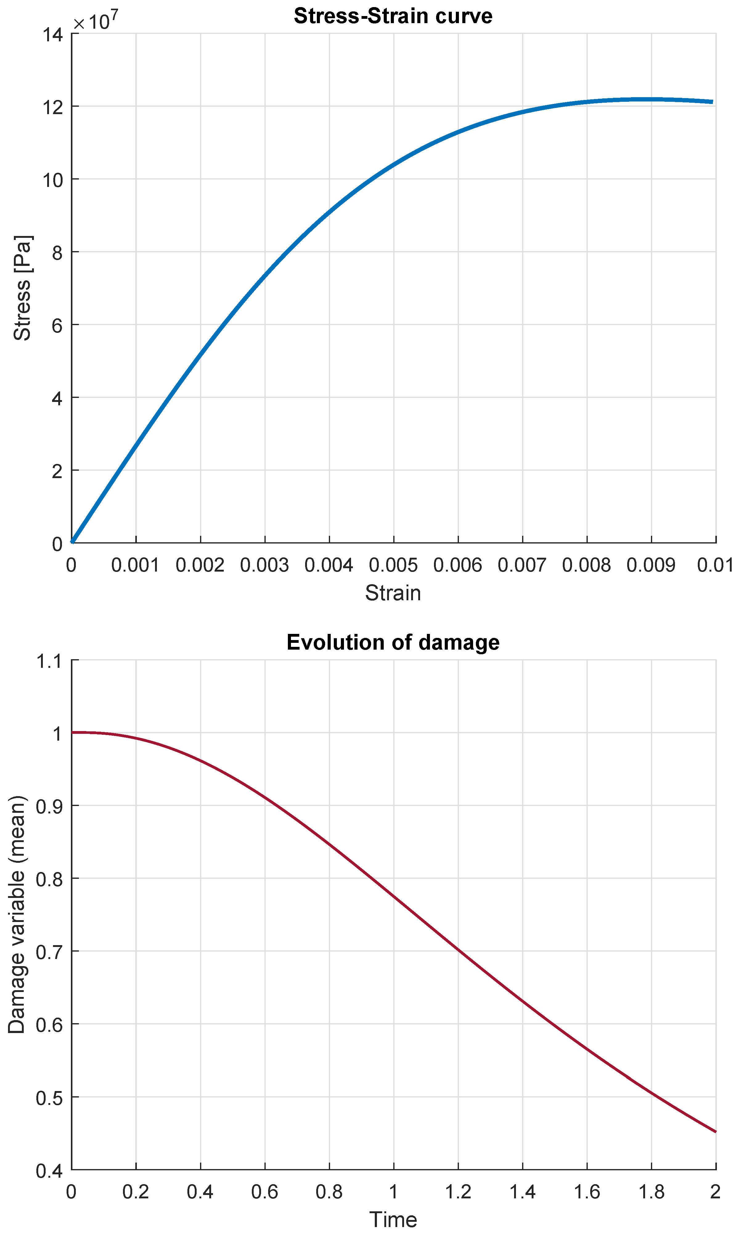
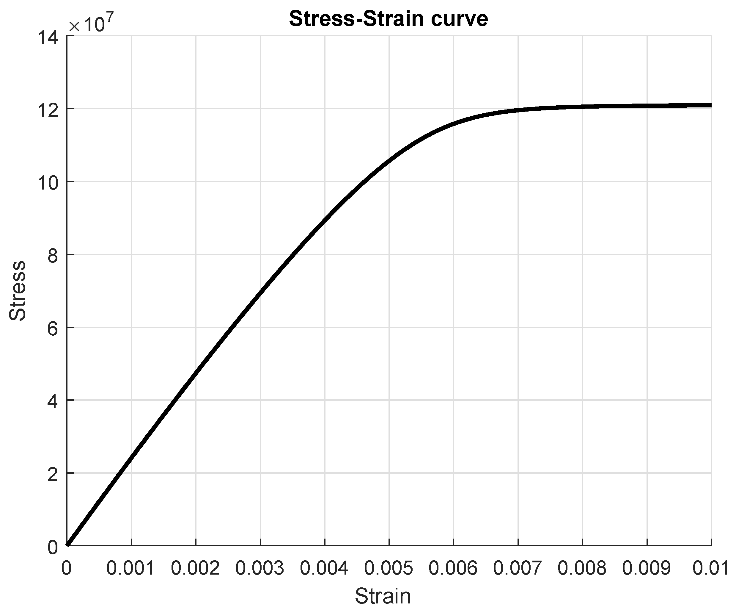
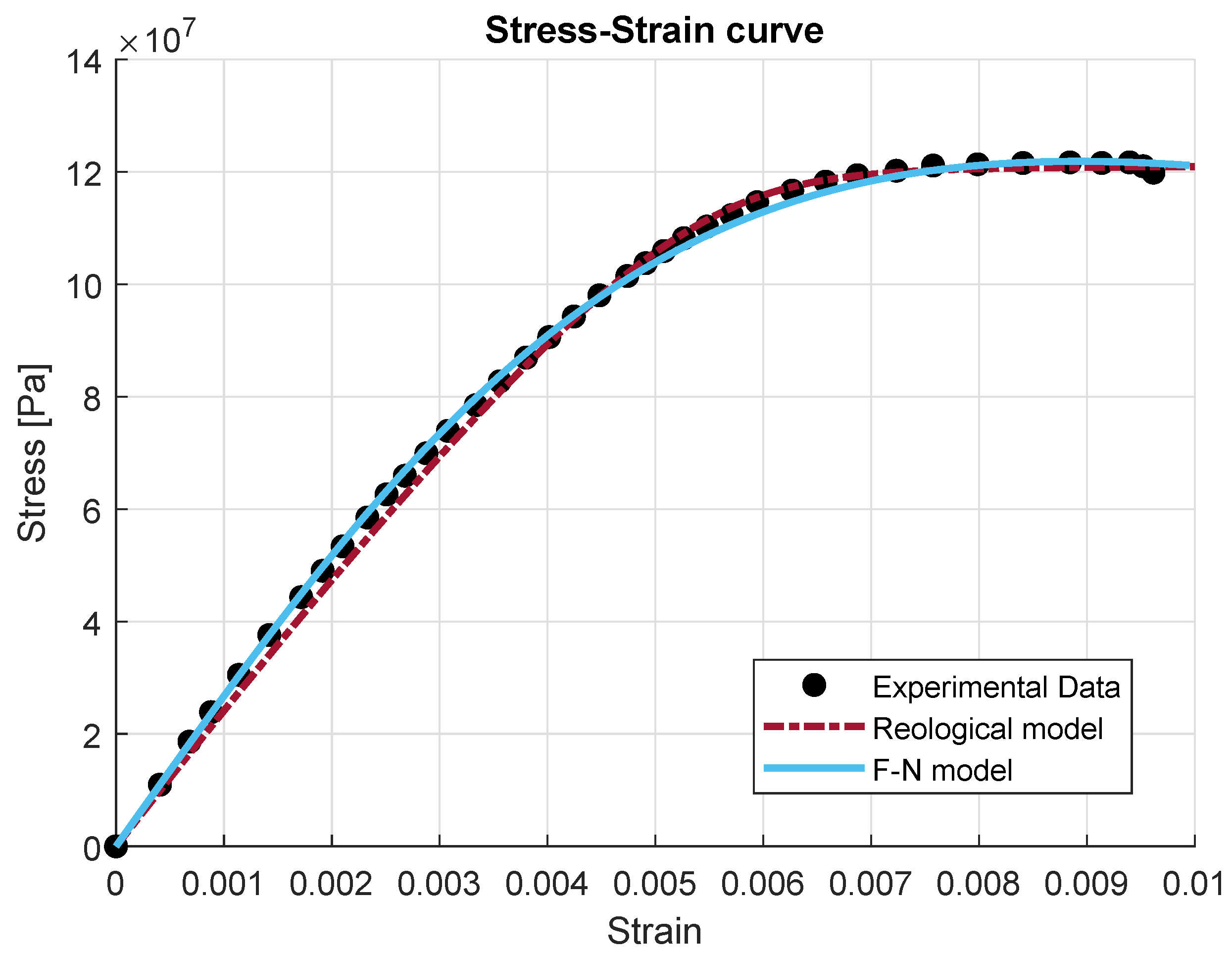
3.1. Comparison in a One-Dimensional Problem

To compare the performance of the models presented in the previous section, a one-dimensional version of both was implemented. To test the models, a typical tensile test was reproduced, since there is experimental data in the literature to evaluate the performance [18]. The one-dimensional model represents a bone fixed on one end and with an increasing displacement imposed on the other end. Stress was computed in postprocessing once the deformation was obtained.
First, we solve the Frémond–Nedjar model with the following data:
T = 2 , Ω = ( 0 , 1 ) , Γ D = { 0 , 1 } , Γ N = , f 0 = 0 , g = 0 , λ = 0 , μ = 1.348 × 10 10 , κ = 0.5 , β = 0.01 , q = 10 5 , λ d = 17 , λ u = 4.2 × 10 5 , λ w = 0 ,
and the initial condition:
β 0 ( x ) = 1 for all x ( 0 , 1 ) .
That is, at initial time we assumed that the bone was completely healed. Moreover, since no mechanical forces were applied, the deformation is produced defining an imposed displacement at the right corner as,
u ( 1 , t ) = 5 × 10 3 · t for all t [ 0 , 2 ] .
We note that the modifications needed to include this case into problem P were really straightforward, so the analysis performed in the previous section could be extended easily.
Using the discretization parameters k = 0.01 and h = 0.05 in Figure 2 (up) the stress–strain curve obtained with the Frémond–Nedjar model is shown. As it can be seen in the evolution of the damage variable (down), the mechanical properties of the bone degrade as the strain increases, leading to the “plastic” region which corresponds with the damage regime of the stress–strain curve.
Secondly, the García et al. model was solved, so in Figure 3 the shape of the stress–strain curve seen before is reproduced again with the rheological model.
Finally, both models were compared with experimental data obtained from [18]. Figure 4 shows the stress–strain curves obtained from both models against the experimental data (black dots). Both models show good agreement with the experimental results, with small differences in the linear part of the curve and the beginning of the damage range. The Frémond–Nedjar model shows better agreement in the linear part, but the curvature of the damage range fits worse than the rheological model. However, these small differences were not significant, since mechanical properties vary greatly from bone to bone, making very accurate fittings not useful.
In any case, both models were capable of reproducing the qualitative characteristics of bone mechanics. In particular, the modified Frémond–Nedjar model shows its capability to be used to model bone tissue in spite of it being proposed to model concrete structures.

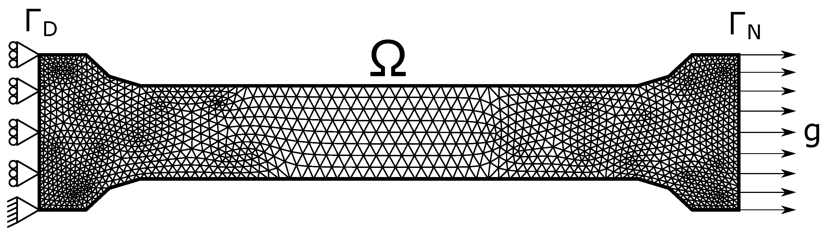
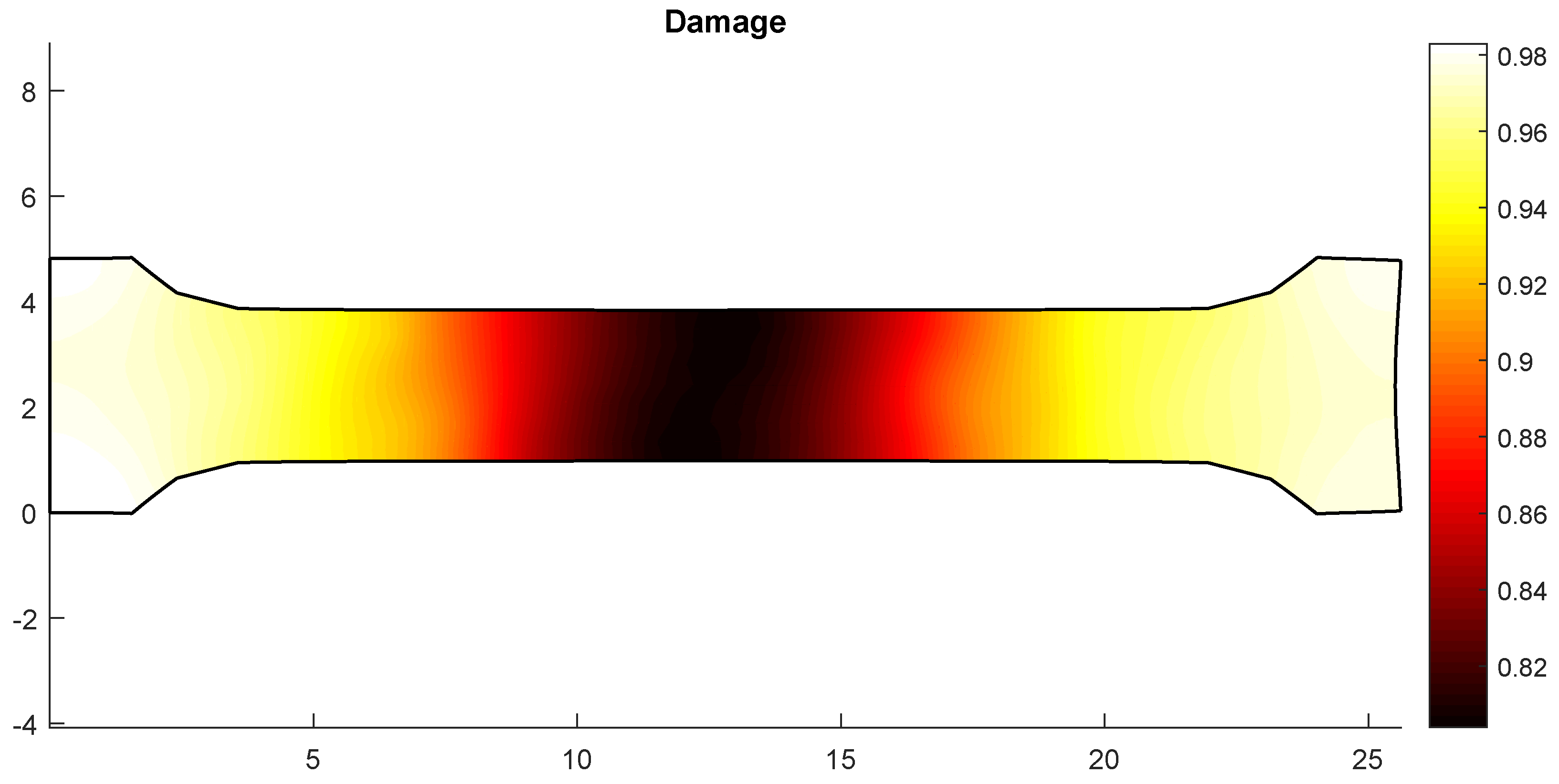
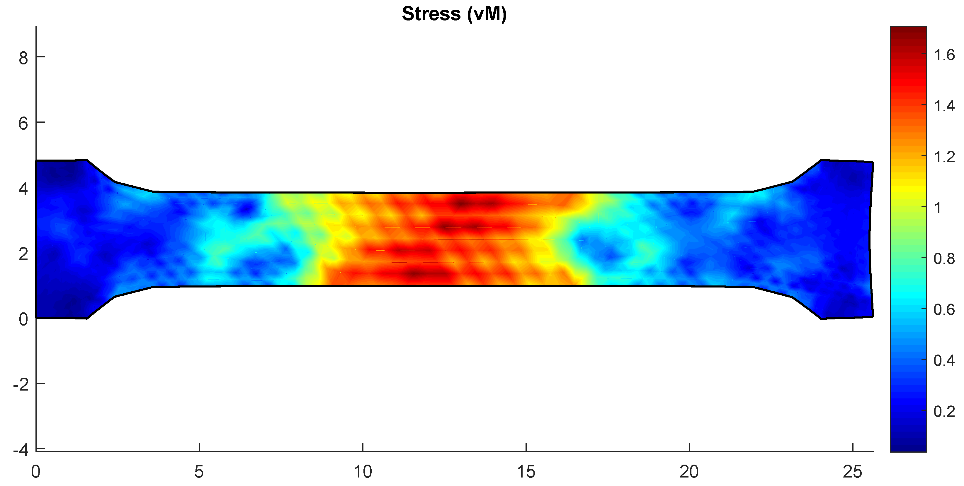
3.2. A Two-Dimensional Problem Solved Using Frémond–Nedjar Model

Now, we consider a two-dimensional case to simulate a more realistic setting. Thus, the bone occupied a two-dimensional domain Ω , which was assumed fixed on its left part Γ D (the whole part clamped on the vertical direction and its lower point also in the horizontal one), and subjected to the action of a surface force on its right part Γ N (see Figure 5).
The following data have been used in this example:
T = 5 , f 0 = 0 , g = ( 5 , 0 ) , λ = 21.1 × 10 10 , μ = 24.61 × 10 10 , κ = 1 , β = 0.01 , q = 10 5 , λ d = 0.01 , λ u = 15 , λ w = 0.0001 ,
and the initial condition:
β 0 ( x , y ) = 1 for all ( x , y ) Ω .
That is, again at initial time we assumed that the bone was completely healed.
Using the time discretization parameter k = 0.1 and the finite element mesh shown in Figure 5, the damage field at final time is plotted over the deformed configuration in Figure 6. As expected, the most damaged areas concentrated in the middle of the bone due to the applied force and the clamping conditions.
Finally, in Figure 7 the stress field is shown at final time over the deformed configuration. We note that now the highest stressed areas concentrated in the middle part of the bone. The concentration of the damage and stress in the middle of the sample agree with the observed fracture of the real probes in uniaxial tests by on middle section.

4. Conclusions

In this work, two ways of modelling damage in cortical bone were studied. The first one was a modification of a well-known damage model for concrete structures, never used for bone tissue. The second one was developed specifically for bone damage and based on a rheological model. One-dimensional simulations were performed to compare both models, reproducing a classical tensile test. Both models show similar solutions and a good agreement with experimental data. Moreover, a two-dimensional example was also considered using the Frémond–Nedjar model to show the behaviour of its solution in a more real situation. The advantage of the use of the Frémond–Nedjar model relies in its formulation, which makes it easier to couple with bone remodelling models, and it allows for a formal numerical analysis. The number of parameters required for this model is also reduced with respect to the García et al. model. These results open the possibility of using this model in bone tissue simulations.

Author Contributions

Conceptualization and Methodology J.B., J.R.F. and A.S.; Software, Formal Analysis and Data Curation J.B. and J.A.L.-C.; Validation J.B., J.R.F. and A.S.; Supervision J.R.F. and A.S.; Writing—Original Draft Preparation J.B. and J.R.F.; Writing—Review and Editing J.A.L.-C. and A.S.; Funding Acquisition J.R.F. and A.S.

Funding

This work has been partially funded by the research project PGC2018-096696-B-I00 (Ministerio de Ciencia, Innovación y Universidades, Spain). J. Baldonedo acknowledges the funding by Xunta de Galicia (Spain) under the program Axudas á etapa predoutoral with Ref. ED481A-2019/230. J.A. López-Campos also acknowledges the funding by Xunta de Galicia (Spain) under the program Axudas á etapa predoutoral with Ref. ED481A-2017/045.

Conflicts of Interest

The authors declare no conflict of interest.

References

  1. Mazars, J. A description of micro- and macroscale damage of concrete structures. Eng. Fract. Mech. 1986, 25, 729–739. [Google Scholar] [CrossRef]
  2. Frémond, M.; Nedjar, B. Damage, gradient of damage and principle of virtual power. Int. J. Solids Struct. 1996, 33, 1083–1103. [Google Scholar] [CrossRef]
  3. Nedjar, B. Elastoplastic-damage modelling including the gradient of damage: Formulation and computational aspects. Int. J. Solids Struct. 2001, 38, 5421–5451. [Google Scholar] [CrossRef]
  4. Wolff, J. The Law of Bone Remodelling; Springer: Berlin/Heidelberg, Germany, 1986. [Google Scholar]
  5. Weinans, H.; Huiskes, R.; Grootenboer, H.J. The behavior of adaptive bone-remodeling simulation models. J. Biomech. 1992, 25, 1425–1441. [Google Scholar] [CrossRef] [Green Version]
  6. Fondrk, M.T.; Bahniuk, E.H.; Davy, D.T. Inelastic strain accumulation in cortical bone during rapid transient tensile loading. J. Biomech. Eng. 1999, 121, 616–621. [Google Scholar] [CrossRef] [PubMed]
  7. Carter, D.R.; Caler, W.E. A cumulative damage model for bone fracture. J. Orthop. Res. 1985, 3, 84–90. [Google Scholar] [CrossRef] [PubMed]
  8. Pattin, C.A.; Caler, W.E.; Carter, D.R. Cyclic mechanical property degradation during fatigue loading of cortical bone. J. Biomech. 1996, 29, 69–79. [Google Scholar] [CrossRef]
  9. Fondrk, M.T.; Bahniuk, E.H.; Davy, D.T. A Damage Model for Nonlinear Tensile Behavior of Cortical Bone. J. Biomech. Eng. 1999, 121, 533–541. [Google Scholar] [CrossRef] [PubMed]
  10. Garcia, D.; Zysset, P.K.; Charlebois, M.; Curnier, A. A 1D elastic plastic damage constitutive law for bone tissue. Arch. Appl. Mech. 2009, 80, 543–555. [Google Scholar] [CrossRef]
  11. Ramtani, S. Damaged elastic bone-column buckling theory within the context of adaptive elasticity. Mech. Res. Commun. 2018, 88, 1–6. [Google Scholar] [CrossRef]
  12. Ramtani, S.; Zidi, M. Damaged-bone remodeling theory: Thermodynamical Approach. Mech. Res. Commun. 1999, 26, 701–708. [Google Scholar] [CrossRef]
  13. Hosseini, H.S.; Horák, M.; Zysset, P.K.; Jirásek, M. An over-nonlocal implicit gradient-enhanced damage-plastic model for trabecular bone under large compressive strains. Int. J. Numer. Methods Biomed. Eng. 2015, 31, e02728. [Google Scholar] [CrossRef] [PubMed]
  14. Martínez, G.; García-Aznar, J.M.; Doblaré, M.; Cerrolaza, M. External bone remodeling through boundary elements and damage mechanics. Math. Comput. Simul. 2006, 73, 183–199. [Google Scholar] [CrossRef]
  15. Mengoni, M.; Ponthot, J.P. An enhanced version of a bone-remodelling model based on the continuum damage mechanics theory. Comput. Methods Biomech. Biomed. Eng. 2015, 18, 1367–1376. [Google Scholar] [CrossRef] [PubMed]
  16. Campo, M.; Fernández, J.R.; Kuttler, K.L.; Shillor, M.; Via no, J.M. Numerical analysis and simulations of a dynamic frictionless contact problem with damage. Comput. Methods Appl. Mech. Eng. 2006, 196, 476–488. [Google Scholar] [CrossRef]
  17. Ciarlet, P.G. Basic error estimates for elliptic problems. In Handbook of Numerical Analysis; Ciarlet, P.G., Lions, J.L., Eds.; North-Holland: Amsterdam, The Netherlands, 1993; Volume II, pp. 17–351. [Google Scholar]
  18. García, D. Elastic Plastic Damage Laws for Cortical Bone. Ph.D. Thesis, Lausanne, École Polytechnique Fédérale de Lausanne, Lausanne, Switzerland, 2006. [Google Scholar]
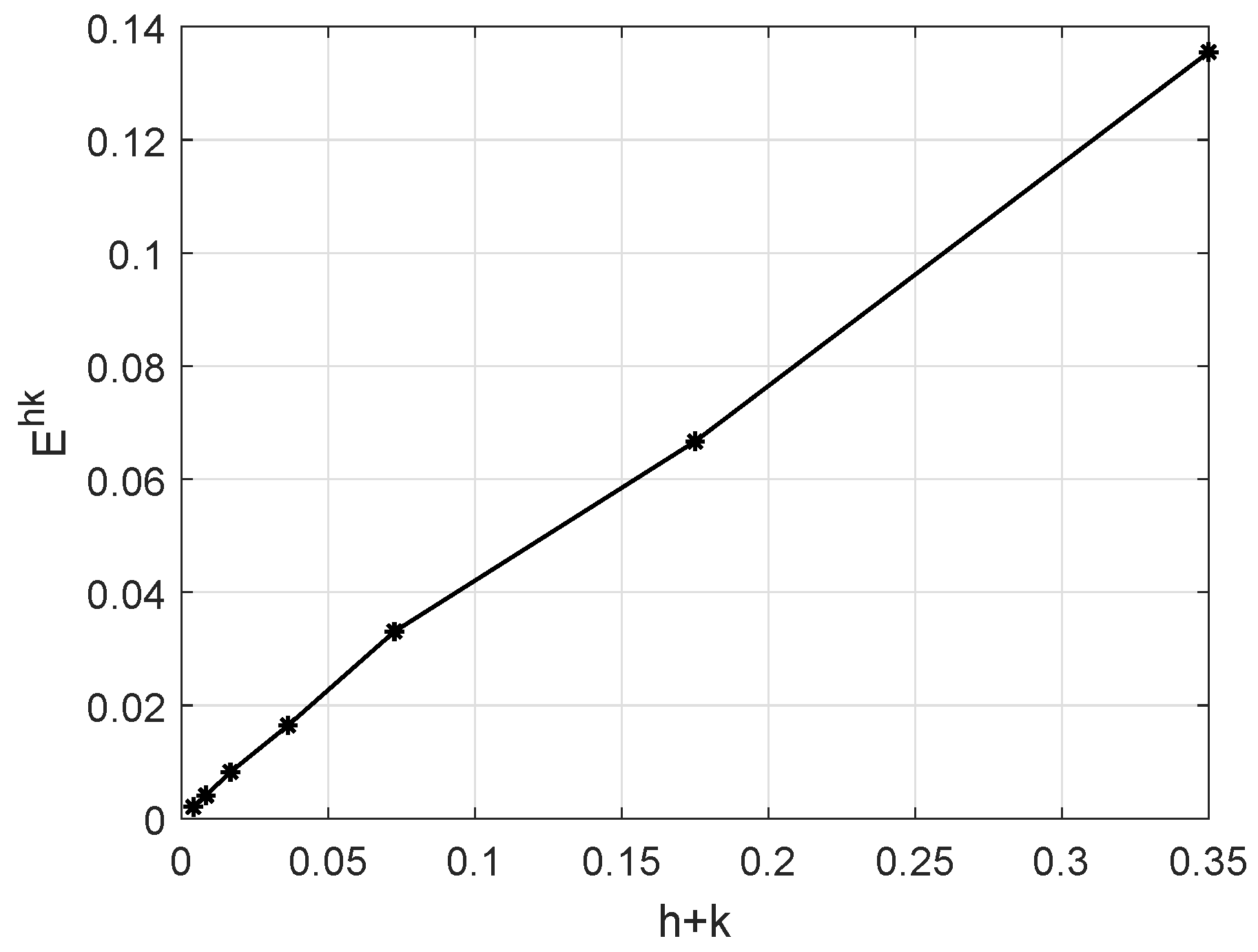
Figure 1. Asymptotic constant error.
Applsci 09 02710 g001
Figure 2. Stress–strain curve obtained with the Frémond–Nedjar model in a tensile test (up) and evolution of the damage variable in the tensile test (down).
Applsci 09 02710 g002
Figure 3. Stress–strain curve obtained with the García et al. model in a tensile test.
Applsci 09 02710 g003
Figure 4. Comparative of both models with experimental data. Source of the experimental data: [18].
Applsci 09 02710 g004
Figure 5. Physical settting and finite element mesh.
Applsci 09 02710 g005
Figure 6. Damage field at final time over the deformed configuration.
Applsci 09 02710 g006
Figure 7. The von Mises stress norm at final time over the deformed configuration.
Applsci 09 02710 g007
Table 1. Numerical errors ( × 100 ) for some discretization parameters.
h k 0.10.010.0010.0001
2 2 13.549013.561313.56126813.561268
2 3 6.65966.66796.6678636.667863
2 4 3.30803.30543.3053863.305386
2 5 1.66411.64571.6456611.645661
2 6 0.84600.82100.8210360.821036
2 7 0.43700.40990.4099420.409942
2 8 0.23280.20460.2045650.204565
2 9 0.13150.10170.1016520.101653
2 10 0.08220.04960.0495970.049596

