Article

Rapid Measurement and Identification Method for the Geometric Errors of CNC Machine Tools

1
State Key Laboratory of Precision Measuring Technology and Instruments, Tianjin University, Tianjin 300072, China
2
Centre of Micro/Nano Manufacturing Technology (MNMT-Dublin), University College Dublin, D04 v1w8 Dublin, Ireland
*
Author to whom correspondence should be addressed.
These authors contributed equally to this work.
Appl. Sci. 2019, 9(13), 2701; https://doi.org/10.3390/app9132701
Submission received: 22 May 2019 / Revised: 22 June 2019 / Accepted: 28 June 2019 / Published: 2 July 2019

Abstract

:
Error compensation technology offers a significant means for improving the geometric accuracy of CNC machine tools (MTs) as well as extending their service life. Measurement and identification are important prerequisites for error compensation. In this study, a measurement system, mainly composed of a self-developed micro-angle sensor and an L-shape standard piece, is proposed. Meanwhile, a stepwise identification method, based on an integrated error model, is established. In one measurement, four degrees-of-freedom errors, including two-dimensional displacement and two-dimensional angle of a linear guideway, can be obtained. Furthermore, in accordance with the stepwise identification method, the L-shape standard piece is placed in three different planes, so that the measurement and identification of all 21 geometric errors can be implemented. An experiment is carried out on a coordinate measuring machine (CMM) to verify the system. The residual error of the angle error, translation error and squareness error are 1.5″, 2 μm and 3.37″, respectively, and these are compared to the values detected by a Renishaw laser interferometer.

1. Introduction

The machining accuracy of CNC MTs decreases with the increase of their service life, the loss of their parts and so on. It is costly to maintain and improve the machining accuracy of MTs by upgrading the hardware. Alternatively, error compensation technology offers a significant means for improving the geometric accuracy of MTs and extending their service life [1]. Modeling, measurement and identification are important prerequisites for geometric error compensation [2]. In recent years, two methods: direct and indirect measurement [3], have focused on the geometric error measurement and identification of MTs.
The direct measurement method involves obtaining all geometric errors directly through the measurement equipment, such as a laser interferometer [4]. Hsieh et al. [5] designed a geometric error measurement system, including one pentaprism module, one PSD module, as well as one laser source, which is capable of obtaining both horizontal and straightness errors in one measurement. However, the system depends on the laser source, so it is necessary to ensure the stability of the laser source during the whole measurement process. In addition, the measurement results are affected by the coupling errors. Gao et al. [6,7] proposed a measurement system, which is mainly composed of two sinusoidal XY-grids and a two-dimensional slope sensor. The simultaneous measurement of five degrees-of-freedom motion, including three-dimensional displacement and a two-dimensional angle, is realized. Nevertheless, there are some disadvantages of the measurement system, such as the complex machining of a sinusoidal angle grid and the nonlinear errors in the displacement measurement.
The indirect measurement method involves obtaining a part of the geometric error through the measurement system, then the remaining geometric errors are decoupled and identified through the integrated error model. The 3-axis MT has 21 geometric error parameters, so the indirect measurement method is widely applied because of its high efficiency. The classical transfer models of geometric errors include the vector method [8], error matrix method [9], rigid body kinematics method [10], multi-body system (MBS) theory [11], and so on. In the practical application environment, any mechanical system can be outlined and abstracted into MBS, so it is widely used in the kinematics analysis and precision modeling of complex mechanical systems, such as robots, MTs and CMM.
Lei et al. [12,13] proposed a new probe-ball device, which is qualified to measure the overall position errors of a five-axis MT. Furthermore, the unknown and not directly measurable link errors can be estimated through the error model. However, due to the contact measurement, the accuracy of its measurement system is affected by the contact deformation, wear and other factors. Du et al. [14] revised the geometric integrated error modeling of 3-axis MTs. Furthermore, the measurement and identification method, based on a cross grid encoder, is proposed. It is suitable for “on machine” measurement. However, this method must be supplemented with a variety of inspection tools, so the detection and installation process is quite complex. The ball board is one of the recommended methods of ISO. Xiang et al. [15] designed a measurement system, a ball–bar test with a 45° wedge, to obtain the systematic geometric error of five-axis MTs. Giacomo et al. [16] proposed a calibration method for the positional errors of CMM, which can be applied in the detection of the linear guideway of MTs as well. It can reduce the cyclic errors by collecting measurement datum in a dynamic mode. Lin et al. [17] shows a compensation method of MTs, according to the error model based on the Abbe principle. However, these systems (Xiang et al. [15], Giacomo et al. [16], Liu et al. [17]) rely on a laser interferometer to identify the geometric error of the linear guideway. However, in practical applications, it has some drawbacks, such as its heavy weight and complicated operation. According to the above-mentioned literature, experts and scholars have conducted a lot of research in the field of the geometric error measurement and identification of MTs in recent years. However, both direct and indirect measurement methods have various shortcomings in practical applications. Nowadays, it is difficult to develop a kind of geometric error measurement and identification system with a high precision and high detection efficiency, as well as easy installation and operation.
In this study, a novel indirect measurement method, based on a stepwise identification method, is proposed. The measurement system was mainly composed of a self-developed micro-angle sensor and an L-shape standard piece. An integrated error model of the 3-axis MTs is established based on the MBS theory. In one measurement, a four degrees-of-freedom error, including two-dimensional displacement and two-dimensional angle of a linear guideway, can be obtained. Furthermore, the decoupling formulas of individual errors are deduced based on the integrated error model. The measurement paths are reasonably planned, and the L-shape standard piece is placed in XOY, XOZ and YOZ. Then, the measurement and identification of all 21 geometric errors can be completed. This study provides a significant basis for error compensation.

2. Integrated Error Model of 3-Axis MTs

2.1. Geometric Error Sources of 3-Axis MTs

The geometric errors of MTs consist of position-dependent geometric errors (PDGEs) and position-independent geometric errors (PIGEs) [18]. For a 3-axis MT, there are three linear guideways. PDGEs are six-dimensional position errors caused by the motion axis, including 3 translation errors and 3 angle errors [19]. Taking the motion of the X-axis as an example, the 6 geometric errors are expressed as δx(x), δy(x), δz(x), εx(x), εy(x), and εz(x) [20]: where δx(x) is the positioning error; δy(x) and δz(x) are the straightness errors; εx(x), εy(x) and εz(x) are the rotations about the x, y and z axes under x motion, which are also called roll, pitch and yaw errors of the X-axis, respectively.
The physical meaning is shown in Figure 1.
PIGEs usually appear as non-parallel, non-vertical or non-intersecting axes. For 3-axis MTs, there are three squareness errors αxy, αxz and αyz between three axes. They do not vary with the motion of its axis. To sum up, the 21 geometric errors of the 3-axis MT are shown in Table 1.

2.2. Structural Analysis of FXYZ 3-Axis MTs

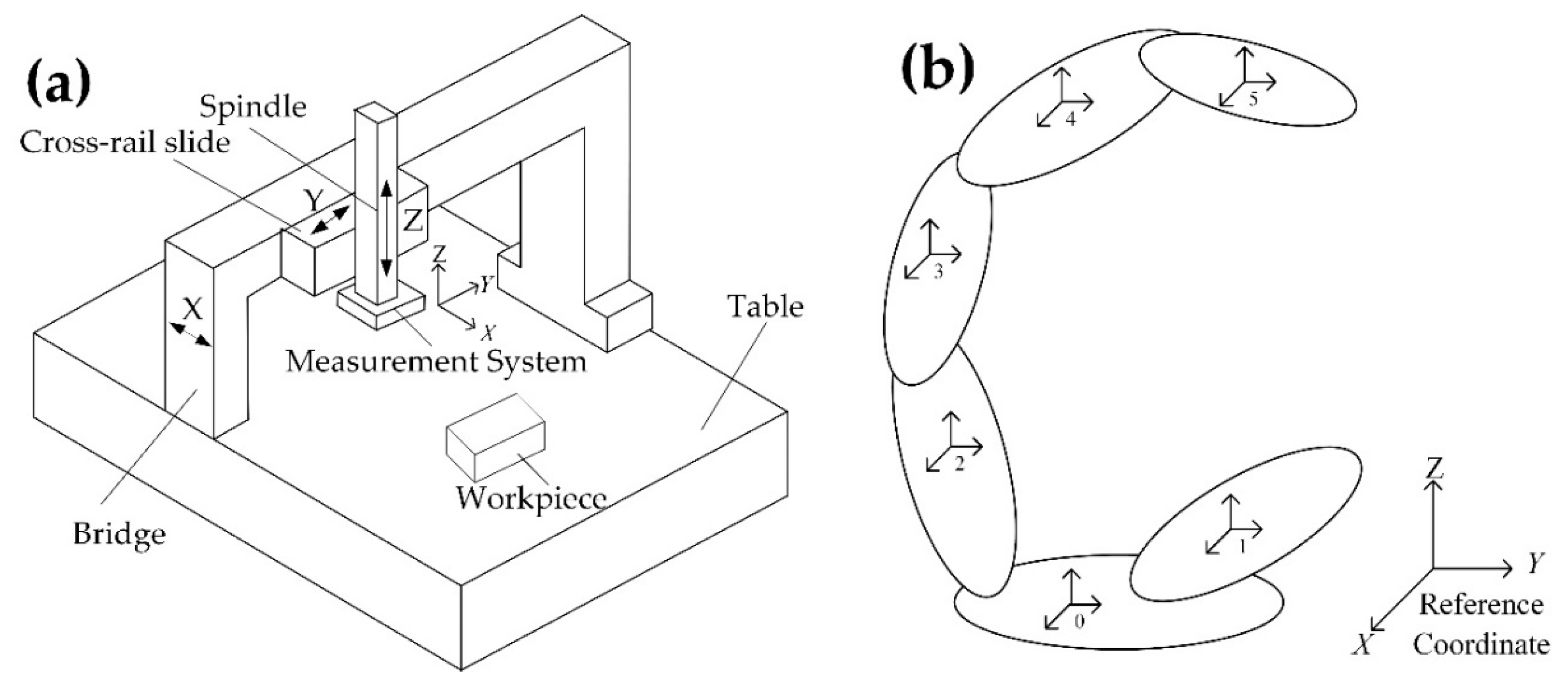
The core of the MBS theory is the analysis of the adjacent bodies and their transformation matrixes, based on the association relation of the topology. The bridge CMM is shown in Figure 2a which can be regarded as a FXYZ 3-axis MT. The bridge moves along the X-axis, the cross-rail slide moves along the Y-axis, and the spindle moves along Z-axis. The topology structure of 3-axis MTs is shown in Figure 2b. The labels 0–5 represents the table, workpiece, X-guideway, Y-guideway, Z-guideway and measurement system, respectively.

2.3. Integrated Error Model of FXYZ 3-Axis MTs

In MBS, the relationship between each adjacent body is transformed into the relationship between adjacent coordinate systems. According to the right-hand rule [21], the worktable coordinate system 00-X0Y0Z0 is established as a reference coordinate system. Then, the coordinate system of the workpiece, X-axis, Y-axis, spindle/Z-axis and measurement system are established as 01-X1Y1Z1, 02-X2Y2Z2, 03-X3Y3Z3, 04-X4Y4Z4, and 05-X5Y5Z5, respectively.
To analyze the geometric error of 3-axis MTs, the coordinate system 0k-XkYkZk (k = 1, 2, 3, 4, 5) is made to coincide with the reference coordinate system in the initial time. The relationship between the coordinate systems can be described by the 4 × 4 homogeneous Denavit-Hartenberg (D-H) matrix. The feature matrix Tij between the body j and the body i can be determined by the nominal motion matrix and error matrix [22]. It is assumed that the initial homogeneous coordinates of the forming point is Pt = [xp yp zp 1]T. When there is nominal motion of the X, Y, and Z axes of the MT, then its actual forming point P and ideal forming point Pw can be obtained as follows:
  P   =   [ 1 ε z ( x ) ε y ( x ) x + δ x ( x ) ε z ( x ) 1 ε x ( x ) δ y ( x ) ε y ( x ) ε x ( x ) 1 δ z ( x ) 0 0 0 1 ] [ 1 α x y 0 0 α x y 1 0 0 0 0 1 0 0 0 0 1 ] [ 1 ε z ( y ) ε y ( y ) δ x ( y ) ε z ( y ) 1 ε x ( y ) y + δ y ( y ) ε y ( y ) ε x ( y ) 1 δ z ( y ) 0 0 0 1 ]   [ 1 0 α x z 0 0 1 α y z 0 α x z α y z 1 0 0 0 0 1 ] [ 1 ε z ( z ) ε y ( z ) δ x ( z ) ε z ( z ) 1 ε x ( z ) δ y ( z ) ε y ( z ) ε x ( z ) 1 z + δ z ( z ) 0 0 0 1 ] [ x p y p z p 1 ]
P w = [ x + x p y + y p z + z p 1 ] T
Then, the integrated error model of FXYZ MT is
E = PPw
The geometric errors of MTs are very small, so the second and higher order errors can be neglected. Moreover, xp = yp = zp = 0 is made to simplify the calculation. Then, Equation (3) is expanded, with only the first-order error remaining, and the integrated error model, represented by 21 error terms, can be expressed as
d x = δ x ( x ) + δ x ( y ) + δ x ( z ) y × ( α x y + ε z ( x ) ) + z × ( α x z + ε y ( y ) + ε y ( x ) )
d y = δ y ( x ) + δ y ( y ) + δ y ( z ) z × ( α y z + ε y ( y ) + ε z ( x ) )
d z = δ z ( x ) + δ z ( y ) + δ z ( z ) + y × ε x ( x ) .
The PDGEs, including translation errors and angle errors, are functions of the motion axis [23]. For example, the angle error εx(x) can be expressed as
ε x ( x ) = f ( x ) = i = 1 n ( r x x i × x i ) = r x x 1 × x + r x x 2 × x 2 + r x x 3 × x 3 + + r x x n × x n
where rxxi (i = 1, 2, …, n) are the coefficients of the fitting polynomial.

3. Measurement Principles

The measurement system is based on the principle of optical auto-collimation and consists of micro-angle sensor and an L-shape standard piece. As shown in Figure 3, the L-shape standard piece is composed of a number of composite modules, which include a plane feature face and rotating paraboloid feature face. During the measurement process, the spindle of the MTs drives the micro-angle sensor to scan the plane surface to obtain its two-dimensional angle. The two-dimensional displacement can be obtained by scanning the rotating paraboloid surface. The array distribution allows the measurement range to expand freely.

3.1. Measurement Principle of the Micro-Angle and Displacement

As shown in Figure 3, the micro-angle sensor, driven by the X-axis of the MT, scans the composite module at the intersection of the L-shape standard piece. Taking the above situation as an example, the measurement principle of the two-dimensional angle and two-dimensional displacement of the motion axis is illustrated.

3.1.1. Measurement Principle of the Micro-Angle

The XOZ section of the measurement system is taken as an example to illustrate the measurement process of the pitch error   ε y ( x ) , as shown in Figure 4.
At the initial time, the angle between the beam and the axis of the composite module in the x direction is α x 0 . The incident beam is emitted to the plane surface, then the reflected beam forms a spot A 0 on the CCD through the convergence of the imaging lenses. As shown in Figure 4a, the position of the image spot does not change when there is a displacement in the x direction between the micro-angle sensor and the composite module. However, when there is a pitch ε y ( x ) , as shown in Figure 4b, the angle between the beam and the axis of the composite module in the x direction changes to α x 1 . Moreover, the imaging point of the reflective beam on the CCD moves from point A 0 to B 0 . Equation (8) can easily be derived:
α x 0 = α x 1 + ε y ( x ) .  
Equation (9) can be derived from the principle of laser collimation [24]:
tan ( 2 α x 1 ) tan ( 2 α x 0 ) = S 1 x S 0 x f
where f is the focal length of the imaging lens, and its value is 100 mm. S0x, S1x is the distance between the center of the spot A0, B0 and the optical axis in the x direction. From Equations (8) and (9), the tangent value is replaced by the angle value due to the measurement of the micro-angle, then the pitch error εy(x) can be expressed as
ε y ( x ) = ( s 1 x s 0 x ) / 2 f
The X-axis drives the micro-angle sensor to scan the plane surface, so that the pitch error εy(xi) of each sampling point, relative to the initial one, can be collected. The least-squares method is used to fit the mean curve of each discrete datum, and the first three terms are selected for the identification study. Then, the pitch error at each point of the composite module surface can be obtained from the following polynomial:
ε y ( x ) = r y x 1 × x + r y x 2 × x 2 + r y x 3 × x 3 lim x
where ryx1, ryx2, and ryx3 are the coefficients of the pitch error polynomial, and x is the nominal motion of the X-axis, which can be obtained from the feedback value of the MT. Considering the structure of the CMM in Figure 2a, a roll error of the X-axis will cause a yaw between the micro-angle sensor and the composite module. Therefore, the roll error εx(x) can be obtained in a similar way by analyzing the Y0Z section of the measurement system. Thus, the pitch and roll error of the X-axis can be separated and measured.
Since it is difficult to know the intersection O of the optical axis and CCD, in the actual measurement process, the spot position on the CCD of the first measurement point is taken as the reference point. By detecting the projection distance between the imaging spots of other measurement points and the reference spot in the x and y direction, respectively, the two-dimensional micro-angle variation of each sampling point, relative to the initial measurement point, can be obtained through Equation (10).

3.1.2. Measurement Principle of Micro-Displacement

Based on the principle of angle measurement, the measurement principle of the displacement is illustrated by the XOZ section of the proposed system, as shown in Figure 5.
The incident beam is emitted to the paraboloid surface, then the reflected beam forms a spot C 0 on the CCD. When the incident beam moves from point C to D, the imaging point of the reflective beam on the CCD moves from point C 0 to D 0 . Equation (12) can be derived from the principle of laser collimation.
tan ( 2 γ x 1 ) tan ( 2 γ x 0 ) = d 1 x d 0 x f
where d0x is the distance between the center of the spot C0 and the optical axis in the x direction, and the distance between the center of the spot D0 and the optical axis in the x direction is d1x.
The surface equation of the rotating paraboloid is
x 2 k 2 + y 2 k 2 = 2 z
where k2 is the characteristic parameter of the rotating paraboloid, and its value is 0.057; and x, y and z represent the three-dimensional coordinates of the measurement point. Then, the tangent slope in the x direction of sampling point C and D can be obtained as follows:
tan ( β x 0 ) = z x = x 0 k 2
tan ( β x 1 ) = z x = x 1 k 2
where x 0 and x 1   are the distance between the sampling point C and D and the center point of the rotating paraboloid. Then, the distance between the sampling points C and D is lx, which can be expressed as
l x = k 2 × ( tan ( β x 1 ) tan ( β x 0 ) ) .
Equation (17) can be derived easily, in accordance with Figure 5:
( β x 1 β x 0 ) = ( γ x 1 ε y ( x 1 ) ) ( γ x 0 ε y ( x 0 ) ) = ( γ x 1 γ x 0 ) ( ε y ( x 1 ) ε y ( x 0 ) )
where ε y ( x 1 ) and ε y ( x 0 )   are the pitch error at the sampling point C and D of the micro-angle sensor, which can be obtained from Equation (11).
From Equations (12), (16), and (17), and the tangent value can be replaced by the angle value for the micro-angle, then the displacement lx can be expressed as
l x = k 2 × ( d 1 x d 0 x 2 f ( ε y ( x 1 ) ε y ( x 0 ) ) )
The displacement in the y direction can be obtained in a similar way by analyzing the Y0Z section of the measurement system. Similar to angle measurement, the two-dimensional displacement variation of each sampling point, relative to the initial one, can be obtained through Equation (18).
In this paper, a CCD detector, with a pixel size of 2.2 μm × 2.2 μm was selected, and 3 times the image segmentation was realized by the image segmentation algorithm. Thus, the resolution δ m   . of the position detection for the imaging spot is 0.73 μm. The convergent lens was used to shrink the laser beam. From the principle of laser collimation, the angle resolution of the micro-angle sensor can be calculated as
δ k = δ m 2 f = 0.76
Then, the displacement resolution can be calculated as
δ s = k 2 × tan δ m 2 f = 0.19   μ m
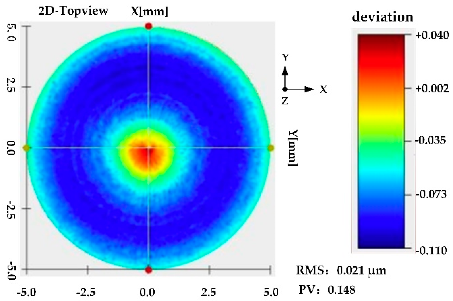
The processing quality of the rotating paraboloid surface is detected by a 3D Surface Measuring system (LuphoScan), as shown in Figure 6. The result shows that the RMS is 0.021 μm. What is more, the PV is 0.148, which indicates that the slope deviation of each point on the rotating paraboloid is within 0.148, compared with the design value. According to Equation (14), its contribution to the measurement accuracy is within 0.008 μm, which can be ignored.

3.2. Implementation of Large-Scale Measurement

The array distribution of the composite modules allows the measurement range to expand freely. However, due to the manufacturing tolerance of the L-shape base, as well as the installation error of each composite module, it is necessary to calibrate the relative position and posture between each composite module. The following is an example of the x direction.
As shown in Figure 7, the composite module at the intersection of the L-shape standard piece is taken as a reference. The relative angle θxi, θyi between each composite module and the reference one, in the direction of x and y, is calibrated. When the micro-angle sensor scans the plane surface i, the two-dimensional angle of each sampling point, relative to the initial one, is εx(xi), εy(xi). Then, the actual angle variation εx(xi), εy(xi) of each point, relative to the initial one, can be calculated:
ε x ( x i ) = ε x ( x i ) θ x i
ε y ( x i ) = ε y ( x i ) θ y i .
The center of the rotating paraboloid is taken as the position reference of each composite module. The relative position (dxi, dyi) between the center of each composite module and the reference one is calibrated. When the micro-angle sensor scans the paraboloid surface i, the two-dimensional displacement of each sampling point, relative to the initial one, is (xi, yi). Then, the actual displacement (xi, yi) of each point, relative to the initial one, can be calculated:
x = x i d x i
y = y i d y i .

4. Stepwise Identification of Geometric Errors

As discussed above, by scanning an arm of the L-shape standard piece, 4 degrees-of-freedom information of the motion axis, including the two-dimensional angle and two-dimensional displacement, can be obtained by the proposed system. In addition, the L-shape layout of the composite modules provides a reference for the measurement of the squareness error. Under the guidance of the integrated error model, the measurement path can be planned reasonably, and then the identification steps for geometric errors are established. For three-axis MTs, by placing the L-shape standard piece in the XOY, XOZ and YOZ planes, the measurement and identification of all 21 geometric errors can be achieved.
The relative positions and postures of each module are calibrated before measurement, taking the standard piece in the XOY plane as an example to illustrate the stepwise identification method of geometric errors.

4.1. Angle Error Identification

As shown in Figure 3, the two arms of the standard piece are placed along the X, Y-axis of the three-axis MT, and the micro-angle sensor is placed along the Z-axis. The X-axis drives the micro-angle sensor to scan each plane surface to measure the roll error εx(xi) and pitch error εy(xi), fitting the mean curve for each discrete datum. Then, the roll and pitch error in the whole measurement range can be obtained from the following polynomial:
ε x ( x ) = r x x 1 × x + r x x 2 × x 2 + r x x 3 × x 3
ε y ( x ) = r y x 1 × x + r y x 2 × x 2 + r y x 3 × x 3
where rxx1, rxx2, and rxx3 are coefficients of the roll error εx(x) polynomial; and ryx1, ryx2, and ryx3 are the coefficients of the pitch error εy(x) polynomial.
Next, the Y-axis drives the micro-angle sensor to scan each plane surface above the other arm of the L-shape standard piece. Considering the structure of the CMM in Figure 2a, this will cause a pitch and yaw between the micro-angle sensor and the composite module when there is a pitch error εx(y) and roll error εy(y) of the Y-axis, respectively. Thus, εx(y) and εy(y) can be measured and their polynomial can be fitted:
ε x ( y ) = r x y 1 × y + r x y 2 × y 2 + r x y 3 × y 3
ε y ( y ) = r y y 1 × y + r y y 2 × y 2 + r y y 3 × y 3
where rxy1, rxy2, and rxy3 are the coefficients of the pitch error εx(y) polynomial; and ryy1, ryy2, and ryy3 are the coefficients of the roll error εy(y) polynomial.
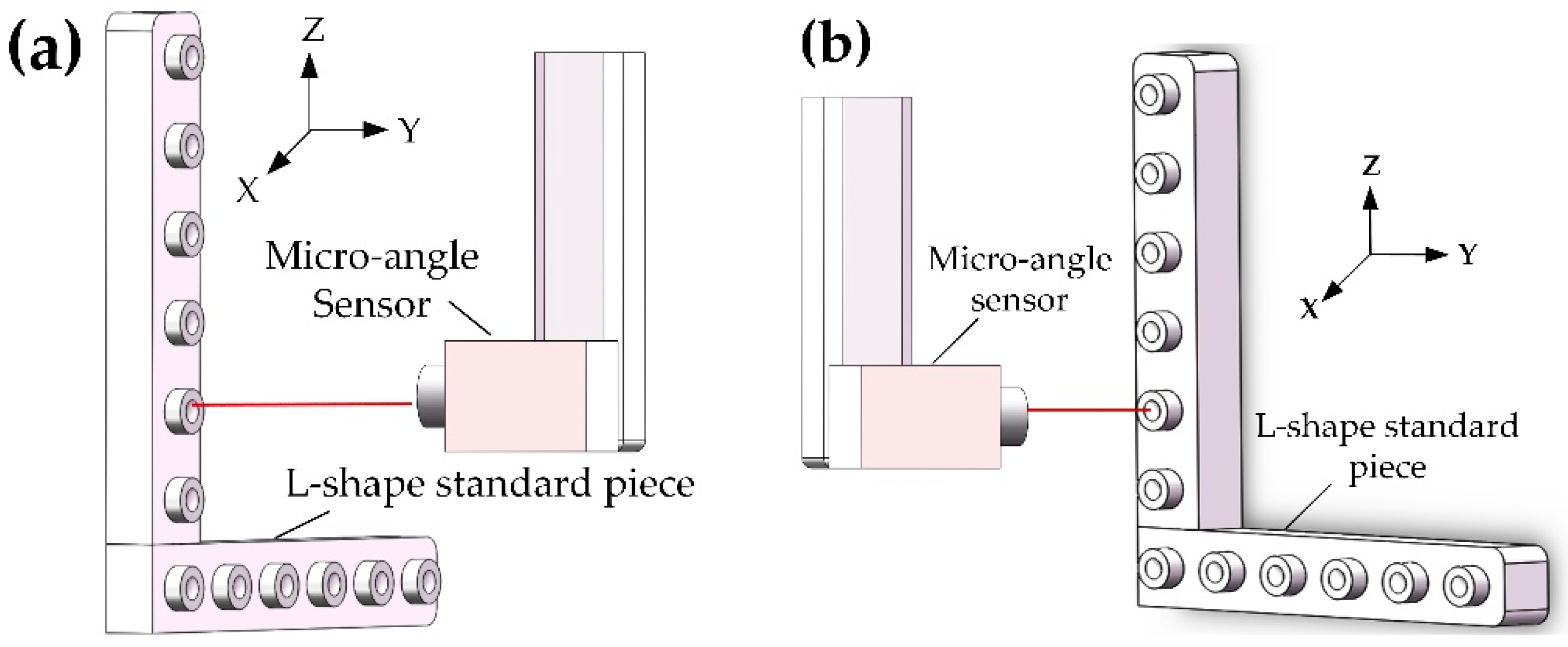
As shown in Figure 8a, the two arms of the standard piece are placed along the X, Z-axis of the MT, and the micro-angle sensor is placed along the Y-axis. The X-axis drives the micro-angle sensor to scan each plane surface. This will cause a yaw between the micro-angle sensor and the composite module, when there is a yaw error εz(x) of the X-axis. Thus, εz(x) can be measured, and its polynomial can be fitted. Then, the Z axis drives the micro-angle sensor to scan each plane surface above the other arm. This will cause a pitch and yaw between the micro-angle sensor and the composite module, when there is a pitch error εx(z) and roll error εz(z) of Z-axis, respectively. Thus, εx(z) and εz(z) can be measured, and their polynomials can be fitted.
At last, as shown in Figure 8b, the two arms of the standard piece are placed along the Y, Z-axis of the MT, and the micro-angle sensor is placed along the X axis. The Y-axis drives the micro-angle sensor to scan each plane surface. This will cause a yaw between the micro-angle sensor and the composite module, when there is a yaw error εz(y) of Y-axis. Thus, the εz(y) can be measured, and its polynomial can be fitted. Then, the Z-axis drives the micro-angle sensor to scan each plane surface above the other arm. This will cause a yaw between the micro-angle sensor and the composite module, when there is a yaw error εy(z) of the Z-axis. Thus, εy(z) can be measured, and its polynomial can be fitted.
To sum up, through the three placements of the L-shape standard piece, the measurement and identification of all 9 angle errors can be implemented.

4.2. Squareness Error Identification

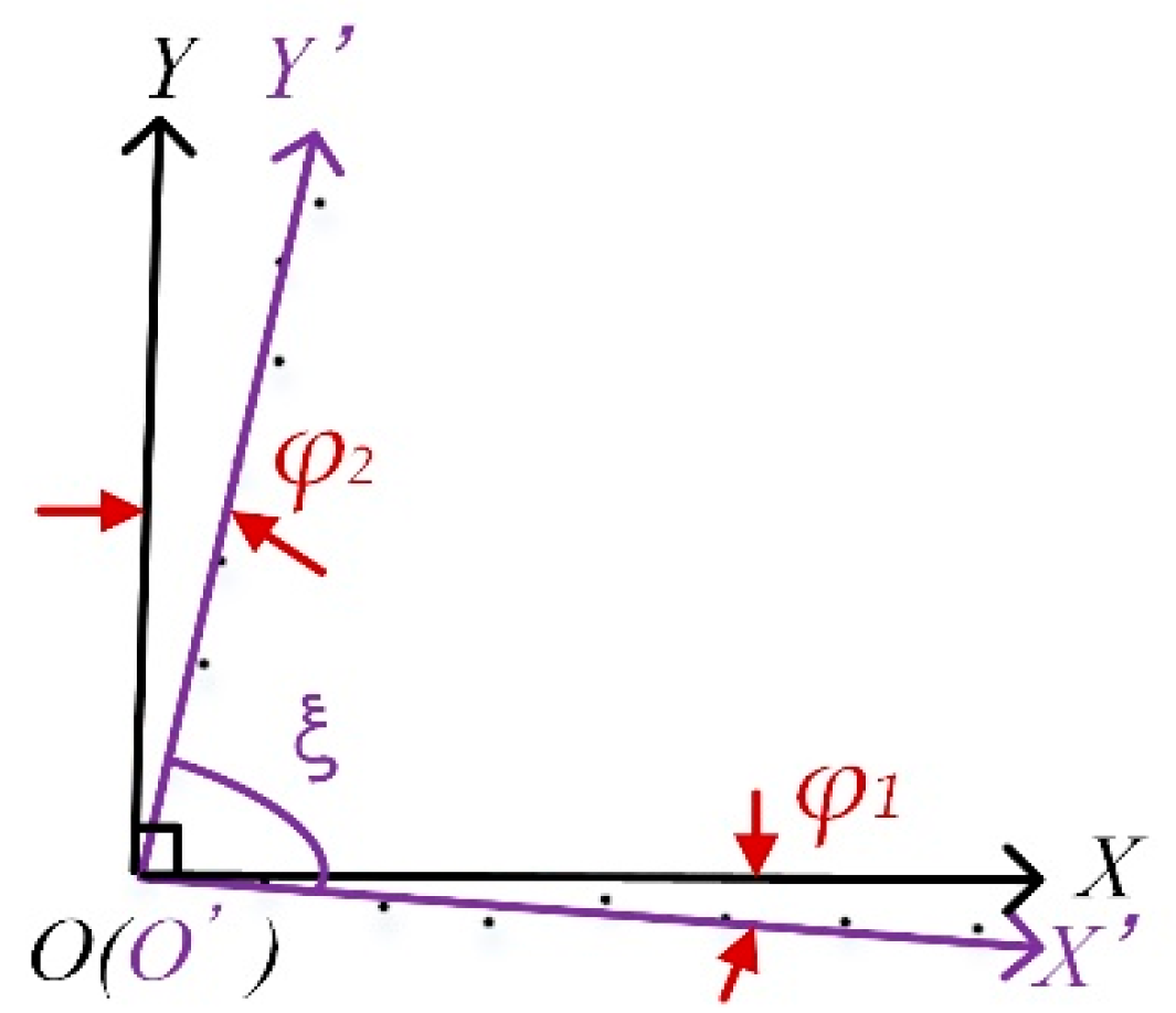
The squareness error between the X and Y-axis is taken as an example. The two-dimensional position coordinates of the initial sampling point A0 are set to be (0, 0). As shown in Figure 3, the X-axis drives the micro-angle sensor to scan each paraboloid surface, and the two-dimensional displacement A1(x1, y1), A2(x2, y2),, Ai(xi, yi) of each sampling point, relative to the initial one, can be obtained, as discussed in Section 3.1.2. As shown in Figure 9, the least-squares method is used to fit the two-dimensional displacement of each sampling point A0, A1, A2,, Ai, and the linear equation of the actual motion path OX’ can be obtained. Then, the Y-axis drives the micro-angle sensor to scan each paraboloid surface, the two-dimensional displacement A1(x1, y1), A2(x2, y2),, Ai(xi, yi) of each sampling point, relative to the initial one, can be obtained, and the linear equation of the actual motion path OY’ is obtained.
As shown in Figure 9, φ 1 is caused by the misalignment of the L-shape line with the X-axis, which can be corrected by software. φ 2 is caused by the misalignment of the L-shape line with the Y-axis and the squareness error of αxy. Obviously, αxy can be calculated as
α x y = φ 2 φ 1
In the actual situation, both the sign and the size relationship of φ 1 and φ 2 are uncertain, while through the linear equation of OX’ and OY’, the angle ξ of the actual motion between the X and Y-axis can be calculated, and α x y can be expressed as Equation (30), without discussing the situations.
α x y = π 2 ξ
Similarly, as shown in Figure 8, the squareness error of αxz and αyz can be derived by placing the L-shape standard piece in the XOZ plane and YOZ plane, respectively.

4.3. Translation Error Identification

The translation errors are decoupled by the integrated error model. By using the fitting polynomial to represent each PDGE, a solvable equation, constituted from Equations (4)–(6), which contains a finite number of unknown coefficients, can be obtained. Furthermore, under the theoretical guidance of the integrated error model, those equations can easily be solved by planning the measurement path reasonably. To put it more concretely, the points on the paraboloid surface are measured when the micro-angle sensor moves along the X-axis, as shown in Figure 3. As discussed in Section 4.2, by subtracting each measured value from the nominal value, the two-dimensional integrated error (dxi, dyi) of each point can be obtained. Then, inputting them into Equations (4)–(6), we find
d x i = δ x ( x i ) + δ x ( y ) + δ x ( z ) y ( α x y + ε z ( x i ) ) + z ( α z x + ε y ( y ) + ε y ( x i ) )
d y i = δ y ( x i ) + δ y ( y ) + δ y ( z ) z ( α z y + ε x ( y i ) + ε x ( x ) )
The Y and Z axes do not move, so the individual errors relative to them will not change at each sampling point. Subtracting the integrated error of any two measurement points to reduce the number of unknown coefficients, we find
d x i d x i 1 = t x x 1 ( x i x i 1 ) + t x x 2 ( x i 2 x i 1 2 ) + t x x 3 ( x i 3 x i 1 3 ) y ( ε z ( x i ) ε z ( x i 1 ) ) + z ( ε y ( x i ) ε y ( x i 1 ) )
d y i d y i 1 = t y x 1 ( x i x i 1 ) + t y x 2 ( x i 2 x i 1 2 ) + t y x 3 ( x i 3 x i 1 3 ) z ( ε x ( x i ) ε x ( x i 1 ) )
where txx1, txx2, and txx3 are the coefficients of the positioning error δx(x) polynomial; tyx1, tyx2, and tyx3 are the coefficients of the straightness error δy(x) polynomial; and xi, y, and z are the nominal motion. What is more, the angle error, such as εy(x), has been identified in Section 4.1. Theoretically, the coefficients of δx(x) and δy(x) of the X-axis can be solved by using the displacement information at 4 sampling points. Then, the fitting polynomial of them can also be obtained:
δ x ( x ) = t x x 1 x + t x x 2 x 2 + t x x 3 x 3
δ y ( x ) = t y x 1 x + t y x 2 x 2 + t y x 3 x 3
Therefore, the positioning error δx(x) and straightness error δy(x) can be identified. Similarly, when the Y-axis moves, the positioning error δy(y) and straightness error δx(y) can be obtained.
As shown in Figure 8a, the X-axis drives the micro-angle sensor to scan each paraboloid surface, so the integrated error of the X-axis in the z direction can be measured, and the polynomial of the straightness error δz(x) can be calculated. Then, the Z-axis drives the micro-angle sensor to scan each paraboloid surface above the other arm, so the integrated error of the Z-axis in the x, z direction can be measured, and the polynomial of δx(z) and δz(z) can be calculated.
At last, as shown in Figure 8b, the Y-axis drives the micro-angle sensor to scan each paraboloid surface, so the integrated error of the Y-axis in the y direction can be measured, and the polynomial of δz(y) can be calculated. Then, the Z-axis drives the micro-angle sensor to scan each paraboloid surface above the other arm, so the integrated error of the Z-axis in the y direction can be measured, and the polynomial of δy(z) can be calculated.
Therefore, all 21 geometric errors can be identified with the stepwise identification method through the three placements of the L-shape standard piece.

5. System Verification

The experiment in the XOY plane was carried out in a CMM, which can be regarded as a FXYZ type of MT. The measurement range in this paper is 200 mm in the direction of x, y and 50 mm between two adjacent composite modules. The relative position and posture between each composite module and the center one are calibrated before measurement.
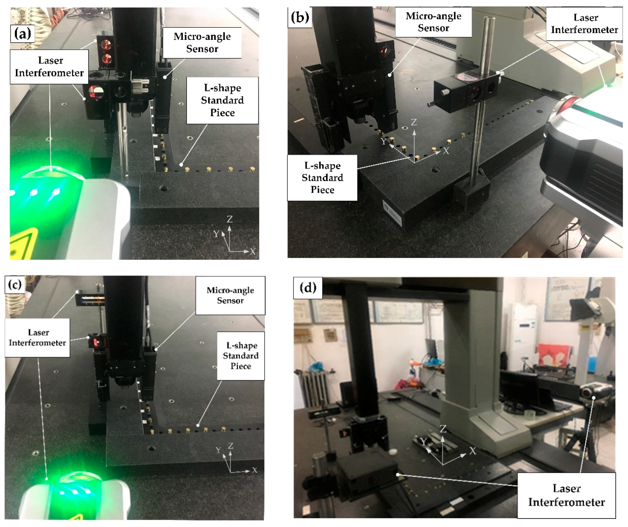
To verify the accuracy of the proposed system, the measurement process is monitored by a Renishaw laser interferometer, whose measurement accuracy of the angle and displacement is 0.1″ and 0.1 μm. The verification setup of the proposed system in the XOY plane is shown in Figure 10. The residual error is defined as the difference between the measurement values of the proposed system and the laser interferometer.

5.1. Angle Measurement

The measurement principle is the same in the two-dimensional angle. While the laser interferometer cannot measure the roll angle, by analyzing the measurement accuracy of the pitch angle, the measurement accuracy of the roll angle can also be obtained. The residual errors of the pitch angle εy(x) and εx(y) are shown in Figure 11. It can be seen that the residual errors are within ±1.5″.
According to the discrete measurement datum measured by the proposed system, Table 2 shows the coefficients of the fitting polynomial of εy(x) and εx(y).

5.2. Displacement Measurement

5.2.1. Squareness Error Identification

The proposed system detects each paraboloid surface in the direction of x and y to acquire the two-dimensional relative displacement of each sampling point. Then, the motion equations in two paths can be obtained by fitting each discrete sampling point using the least-squares method. The slope of the regression linear of the motion equation in the x, y direction is 878.009 (μm/m) and 534.5027 (μm/m), respectively. The squareness error is calculated to be 71.6″. However, it is 68.23″, measured by the laser interferometer. Thus, the residual error of the squareness error is calculated to be 3.37″.

5.2.2. Translation Error Identification

The laser interferometer can detect only one error at a time. Therefore, as shown in Figure 10, the measurement experiment of the displacement must be carried out twice, so that the laser interferometer can monitor the positioning error and the straightness error.
According to the identification method in Section 4.3, Table 3 shows the coefficients of the fitting polynomials of the positioning error and straightness error of the X, Y axis, respectively.
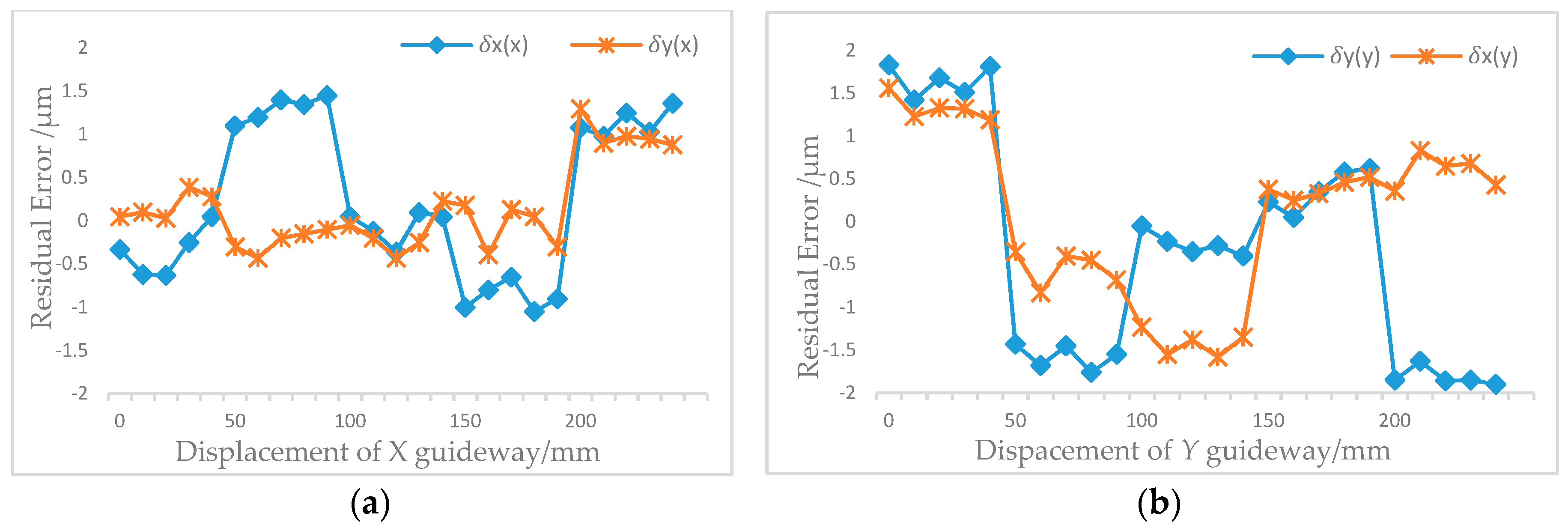
The discrete datum for the positioning errors at each sampling point can be obtained by inputting the feedback value of MT into the polynomial. Figure 12 shows the residual errors of the translation errors, including positioning errors δx(x) and δy(y) and the straightness errors δy(x) and δx(y) at each sampling point. It can be seen that the identification error of the translation errors is within ±2 μm.

6. Conclusions

In this study, a novel indirect measurement method, based on stepwise identification, has been proposed. The proposed system is mainly composed of a self-developed micro-angle sensor and an L-shape standard piece. An integrated error model of 3-axis MTs is established, based on the MBS theory. In one measurement, four degrees-of-freedom errors, including the two-dimensional displacement and two-dimensional angle of a linear guideway, can be obtained. The discrete datum of the angle errors is fitted by the least-squares method in order to obtain the errors in the whole measurement range, which also facilitates the decoupling of translation errors. Furthermore, the L-shape standard piece is placed in three different planes, so that the measurement and identification of all 21 geometric errors can be implemented.
The features of the proposed system in this paper are summarized as follows:
(a)
The four degrees-of-freedom errors can be obtained in one measurement;
(b)
Owing to the L-shape layout of the standard piece, the proposed system is capable of measuring the squareness error between two linear guideways;
(c)
The translation errors, including positioning errors and straightness errors, are decoupled by the integrated error model;
(d)
The residual error of the angle error, translation error and squareness error are 1.5″, 2 μm and 3.37″ and are compared to those detected by a Renishaw laser interferometer.

Author Contributions

X.L., F.F. and X.Y. proposed the measurement system as well as the stepwise identification method. X.L. and F.F. designed the experiments and modified the paper. X.W., Z.L., J.L. and H.L. helped X.Y. perform the experiments. L.G. and Z.S. developed the system software. X.Y. analyzed the datum and wrote the paper.

Funding

The authors express their gratitude to the Science Foundation Ireland (SFI) (No. 15/RP/B3208) and National Natural Science Foundation of China (NSFC) (Nos. 51320105009 & 61635008) for their support.

Conflicts of Interest

The authors declare no conflict of interest.

References

  1. Tian, W.J.; Guo, L.Z. Rapid Identification Method for Geometric Errors of CNC Machine Tools. J. Tianjin Univ. (Sci. Technol.) 2016, 49, 171–177. [Google Scholar]
  2. Han, F.; Zhao, J.; Zhang, L. Synthetical Analysis and Experimental Study of the Geometric Accuracy of CNC Machine Tools. J. Mech. Eng. 2012, 48, 141–148. [Google Scholar] [CrossRef]
  3. Hong, M.; Su, H.; Li, Z.; Wei, Y. Error motion diagnosis of NC machine tools, comment and countermeasure. Chin. J. Mech. Eng. 2002, 38, 90–94. [Google Scholar] [CrossRef]
  4. Ikram, M.; Hussain, G. Michelson interferometer for precision angle measurement. Appl. Opt. 1999, 38, 113–120. [Google Scholar] [CrossRef] [PubMed]
  5. Hsieh, T.; Chen, P.; Jywe, W.; Chen, G.; Wang, M. A Geometric Error Measurement System for Linear Guideway Assembly and Calibration. Appl. Sci. 2019, 9, 574. [Google Scholar] [CrossRef]
  6. Gao, W.; Saito, Y.; Sato, H. Development of a Sensitive Two-Axis Micro-Angle Sensor. J. Jpn. Soc. Precis. Eng. Contrib. Pap. 2006, 72, 1174–1178. [Google Scholar] [CrossRef] [Green Version]
  7. Gao, W.; Kimura, A. A Three-axis Displacement Sensor with Nanometric Resolution. CIRP Ann. 2007, 56, 529–532. [Google Scholar] [CrossRef]
  8. Weckenmann, A.; Estler, T.; Peggs, G. Probing systems in dimensional metrology. CIRP Ann. Manuf. Technol. 2004, 53, 657–684. [Google Scholar] [CrossRef]
  9. Donmez, M.A.; Blomquist, D.S.; Hocken, R.J.; Liu, C.R.; Barash, M.M. A general methodology for machine tool accuracy enhancement by error compensation. Precis. Eng. 1986, 8, 187–196. [Google Scholar] [CrossRef]
  10. Paraskevopoulos, E.; Natsiavas, S. A new look into the kinematics and dynamics of finite rigid body rotations using Lie group theory. Int. J. Solids Struct. 2013, 50, 57–72. [Google Scholar] [CrossRef] [Green Version]
  11. Khan, A.W. Systematic Geometric Error Modeling for Workspace Volumetric Calibration of a 5-axis Turbine Blade Grinding Machine. Chin. J. Aeronaut. 2010, 23, 604–615. [Google Scholar] [CrossRef] [Green Version]
  12. Lei, W.T.; Hsu, Y.Y. Accuracy test of five-axis CNC machine tool with 3D probe–ball. Part I: Design and modeling. Int. J. Mach. Tools Manuf. 2002, 42, 1153–1162. [Google Scholar] [CrossRef]
  13. Lei, W.T.; Hsu, Y.Y. Accuracy test of five-axis CNC machine tool with 3D probe-ball. Part II: Errors estimation. Int. J. Mach. Tools Manuf. 2002, 42, 1163–1170. [Google Scholar] [CrossRef]
  14. Du, Z.; Zhang, S.; Hong, M. Development of a multi-step measuring method for motion accuracy of NC machine tools based on cross grid encoder. Int. J. Mach. Tools Manuf. 2010, 50, 270–280. [Google Scholar] [CrossRef]
  15. Xiang, S.; Li, H.; Deng, M.; Yang, J. Geometric error identification and compensation for non-orthogonal five-axis machine tools. Int. J. Adv. Manuf. Technol. 2018, 96, 2915–2929. [Google Scholar] [CrossRef]
  16. Giacomo, B.; Morais, C.A. Calibration of Positional Errors in Coordinate Measuring Machines and Machine Tools Using a Laser Interferometer System. Appl. Mech. Mater. 2015, 798, 303–307. [Google Scholar] [CrossRef]
  17. Liu, H.; Xiang, H.; Chen, J.; Yang, R. Measurement and compensation of machine tool geometry error based on Abbe principle. Int. J. Adv. Manuf. Technol. 2018, 98, 2769–2774. [Google Scholar] [CrossRef]
  18. Zhu, S.; Dinga, G.; Jiang, L.; Li, Z.; Yana, K. Integrated geometric error modeling, identification and compensation of CNC machine tools. Int. J. Mach. Tools Manuf. 2012, 52, 24–29. [Google Scholar] [CrossRef]
  19. Chen, J.; Lin, S.; He, B. Geometric error compensation for multi-axis CNC machines based on differential transformation. Int. J. Adv. Manuf. Technol. 2014, 71, 635–642. [Google Scholar] [CrossRef]
  20. Cao, L.; Zhong, J.L.; Jie, M.I. Space Geometry Error Modeling for Five-Axis NC Machine Tools Based on Multi-Body System Kinematics. Mech. Res. Appl. 2014, 27, 33–36. [Google Scholar]
  21. Zhong, G.; Wang, C.; Yang, S.; Zheng, E.; Ge, Y. Position geometric error modeling, identification and compensation for large 5-axis machining center prototype. Int. J. Mach. Tools Manuf. 2015, 89, 142–150. [Google Scholar] [CrossRef]
  22. Su, S.P.; Li, S.Y. A Universal Synthetic Volumetric Error Model of Multi-axis NC Machine Tool Based on Kinematics. J. Natl. Univ. Def. Technol. 2001, 23, 45–50. [Google Scholar]
  23. Bi, Q.; Huang, N.; Chao, S.; Wang, Y.; Zhu, L.; Han, D. Identification and compensation of geometric errors of rotary axes on five-axis machine by on-machine measurement. Int. J. Adv. Manuf. Technol. 2016, 84, 505–512. [Google Scholar] [CrossRef]
  24. Fang, F.Z.; W., Y. Three-Dimensional Displacement Measurement System Based on Optical Free-Form Surface. J. Tianjin Univ. (Sci. Technol.) 2014, 47, 934–940. [Google Scholar]
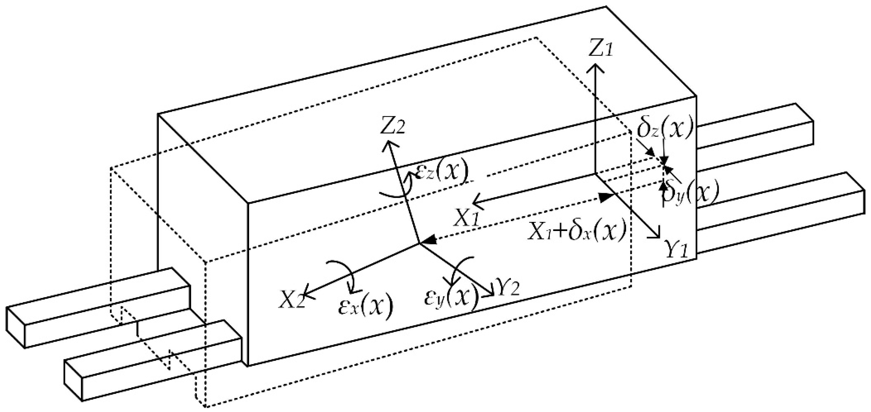
Figure 1. The six geometric errors of the X axis.
Applsci 09 02701 g001
Figure 2. (a) Schematic diagram of the bridge CMM; (b) Topology structure of 3-axis MTs.
Applsci 09 02701 g002
Figure 3. Composition of the measurement system.
Applsci 09 02701 g003
Figure 4. XOZ section of the measurement system, when detected at the plane surface: (a) The micro-angle sensor has a displacement in the X direction; (b) The micro-angle sensor has a pitch error   ε y ( x ) .
Applsci 09 02701 g004
Figure 5. XOZ section of the measurement system, when detected at the rotating paraboloid surface.
Applsci 09 02701 g005
Figure 6. Test results of the rotating paraboloid, detected by LuphoScan.
Applsci 09 02701 g006
Figure 7. Implementation of large-scale measurement.
Applsci 09 02701 g007
Figure 8. (a) Measurement in the XOZ plane; (b) Measurement in the YOZ plane.
Applsci 09 02701 g008
Figure 9. The identification principle of the squareness error.
Applsci 09 02701 g009
Figure 10. Verification setup of the proposed system in the XOY plane: (a) Angle comparison experiment; (b) Positioning error comparison experiment; (c) Straightness error comparison experiment; (d) Squareness error measured by the laser interferometer.
Applsci 09 02701 g010
Figure 11. Residual errors of the proposed system: (a) Residual error of εy(x); (b) Residual error of εx(y).
Applsci 09 02701 g011
Figure 12. Residual errors of the proposed system: (a) Residual error of δx(x) and δy(y); (b) Residual error of δy(x) and δx(y).
Applsci 09 02701 g012
Table 1. The 21 geometric error sources of the 3-axis MTs.
AxisPDGEsPIGEs
X δx(x) δy(x) δz(x) εx(x) εy(x) εz(x)
Y δx(y) δy(y) δz(y) εx(y) εy(y) εz(y)αxy
Z δx(z) δy(z) δz(z) εx(z) εy(z) εz(z)αxz αyz
Table 2. Coefficients of εy(x) and εx(y).
(Arcsec/MM)The First Order The Second OrderThe Third Order
εy(x)−1.01 × 10−22.59 × 10−5−6.50 × 10⁻⁸
εx(y)−3.29 × 10−31.44 × 10−4−4.53 × 10⁻⁷
Table 3. Coefficients of the translation errors.
(μm/mm)First Order Second Order Third Order
δx(x)−1.18 × 10⁻²−3.99 × 10−41.95 × 10−6
δy(x)1.42 × 10⁻¹−1.19 × 10−32.48 × 10−6
δy(y)8.60 × 10⁻³−1.42 × 10−38.42 × 10−6
δx(y)9.47 × 10⁻²−2.01 × 10−39.46 × 10−6