Individualized Interaural Feature Learning and Personalized Binaural Localization Model ^†

Abstract

The increasing importance of spatial audio technologies has demonstrated the need and importance of correctly adapting to the individual characteristics of the human auditory system, and illustrates the crucial need for humanoid localization systems for testing these technologies. To this end, this paper introduces a novel feature analysis and selection approach for binaural localization and builds a probabilistic localization mapping model, especially useful for the vertical dimension localization. The approach uses the mutual information as a metric to evaluate the most significant frequencies of the interaural phase difference and interaural level difference. Then, by using the random forest algorithm and embedding the mutual information as a feature selection criteria, the feature selection procedures are encoded with the training of the localization mapping. The trained mapping model is capable of using interaural features more efficiently, and, because of the multiple-tree-based model structure, the localization model shows robust performance to noise and interference. By integrating the direct path relative transfer function estimation, we propose to devise a novel localization approach that has improved performance in the presence of noise and reverberation. The proposed mapping model is compared with the state-of-the-art manifold learning procedure in different acoustical configurations, and a more accurate and robust output can be observed.

1. Introduction

Spatial audio technologies has shown its importance in various fields, such as video conferencing, virtual reality, humanoid robot interactions and hearing aids, and there are many existing methods reproducing a spatial sound field on different devices for human listeners. To adapt those devices for great spatial experiences, it is necessary to find the most valuable acoustic cues for human hearing system [1,2,3,4]. Additionally, testing and evaluating the quality of reproduced sound field and the hearing experience of those devices is another challenging problem [5,6,7]. The hearing tests with real human volunteers can be time-consuming and would be unfeasible for a huge amount of devices and testing scenarios. One efficient solution is building binaural localization models based on the study of human audio localization mechanism, then running tests on the model for evaluation [8].

Much behavioural and psychoacoustic evidence has confirmed that two individualized interaural cues, Interaural Time Difference (ITD) and Interaural Level Difference (ILD), play an essential role in localizing a sound source. Through intensive studies of the human hearing mechanism, it has become widely understood that individualized ITD and ILD are mainly determined by the filtering of the head, body and pinna, where the filtering function is the so-called Head-Related Transfer Function (HRTF). During the last two decades, many binaural localization approaches have been developed based on interaural cues. Li and Levinson [9] adopted the Bayes rule to estimate the source position. This method uses interaural intensity difference (IID) and spectral signals to refine the initial estimate given by ITD. Viste et al. [10] provided an individual parametric model jointly using ILD and ITD for azimuth localization. The model first provides a rough estimate of high standard variation based on ILD, and then refines the estimation by selecting the closest ITD. Woodruff and Wang combined ILD and ITD with a Gaussian Mixture Model (GMM), which also embedded the environmental condition as a latent parameter [11].

Further, many works have attempted to investigate the relationship between interaural cues and source position in a 3-D space. Duba summarized the relationship between interaural cues and azimuth/elevation [12]. Keyrouz et al. proposed a maximum cross-correlation matching method in source cancellation algorithms to pinpoint the source location in a 3-D space [13,14]. Liu et al. introduced a Bayesian rule-based hierarchical localization system using IID time delay compensation and an interaural matching filter to estimate azimuth and elevation in the interaural-polar coordinate system [15,16]. Deleforge et al. proved the local linear bijective mapping between interaural cues and source location on the binaural manifold, and derived a statistical localization model using an EM algorithm [17,18]. Weng et al. adopted a non-parametric tree-based learning method to retrieve the mapping between the interaural cues and source locations with fewer restrictions on its spatiotemporal characteristics and environment structure [19].

Several studies mentioned above have demonstrated the importance of feature spectrum selection to localization performance, especially for elevation localization, and various methods for feature selection have been proposed. Duba et al. indicated that the IID at the frequency above 2 kHz contains the characteristics of head shadow and pinna diffraction [12], which can be exploited for elevation estimation. Algazi et al. retrieved the existence of elevation-dependent features at a low frequency, which was attributed to head diffraction and torso reflections [20]. Deleforge et al. proved the elevation ambiguities of Interaural Phase Difference (IPD) at the high-frequency range (between 2 to 8 kHz) and used a feature space concatenated by full-spectrum ILD and low-frequency IPD [17].

Another challenge in sound source localization is localizing the source in the presence of noise and reverberation. There have been many attempts to obtain the interaural features in a complex environment and diminish the effects of room reverberation and background noise [21,22,23]. However, prior knowledge of the room’s acoustical characteristics is required for most of those methods, and, without this prior knowledge, the extracted interaural features may not be optimized and some interference would be retained. Therefore, a model with high tolerance to noise and these interferences would be expected for practical applications.

This article investigates the dependency between interaural features and sound source position, particularly for elevation mapping. The Mutual Information (MI) is used to demonstrate the existence of elevation-related dependency on both the ILD and IPD spectrum. Then, based on the results of the MI analysis, a chain rule-based probabilistic model for mapping the features and source locations in a 3-D space is proposed. The model is constructed based on probability estimation trees (PETs) and Random Forest (RF) framework. The PETs are formed by an information gain–based data partition technique. The features exploited by the model are further investigated, which justifies that the non-linear-dependent features (e.g., high-frequency IPD spectrum) can also contribute to an accurate localization performance. Then, aiming at evaluating the accuracy and robustness of the proposed method, the localization performances are compared with the state-of-the-art probabilistic piecewise affine mapping (PPAM) model proposed in [17] in different noise and reverberation environments without prior knowledge of the acoustical conditions.

2. Individualized Feature Selection Using Mutual Information

Firstly, we focus on selecting the most valuable spatial cues and their mapping relationship to the source position. Considering a complex environment, the additive noise and reverberations would distort the characteristics of both the phase and magnitude features, especially at higher frequencies (above 3 kHz) where the speech energy is comparatively low. This is exacerbated, as most elevation localization cues being generated by reflections and diffraction of the human body and pinna are above 3 kHz [24]. Therefore, a feature selection mechanism that maximizes the direction-dependent information and minimizes the effect of noise would be necessary, and a generic feature selection approach could lead to superior performance [25]. To investigate the dependency between the features and their corresponding source positions, the Mutual Information (MI) that exists between each spatial localization cue and the source location for particular feature spectra could be used as criteria to evaluate both the effectiveness and robustness of the feature vectors extracted for the localization process.

We assume the left and right ear received signals are modeled in time-frequency (T-F) domain as:

$$\begin{array}{c}{X}_{\mathrm{l},k,f}=H_{\mathrm{l},\mathrm{f}}(\vartheta ,\phi )·S_{k,f}+N_{\mathrm{l},k,f}\hfill \\ X_{\mathrm{r},k,f}=H_{\mathrm{r},\mathrm{f}}(\vartheta ,\phi )·S_{k,f}+N_{\mathrm{r},k,f}\hfill \end{array}$$

(1)

where k and f indicate the time frame index and frequency index, respectively. The S represents the source signal, and $H_{\mathrm{l},\mathrm{f}}$ and $H_{\mathrm{r},\mathrm{f}}$ denotes the relative transfer function with spatial parameters ${\Theta }_{\mathrm{IP}}=(\vartheta ,\phi )$ in the interaural-polar coordinate system [24]. $N_{\mathrm{l},k,f}$ and $N_{\mathrm{r},k,f}$ denotes the additive random background noise. The interaural cues IPD and ILD at frequency f are obtained by:

$$\begin{array}{c}{v}_f^p=\angle \left|\frac{X_{\mathrm{l},k,f}}{X_{\mathrm{r},k,f}}\right|\\ v_f^m=20{log}_{10}\left|\frac{X_{\mathrm{l},k,f}}{X_{\mathrm{r},k,f}}\right|\end{array}$$

(2)

Then, we organize the interaural phase and magnitude feature vector as:

$$\begin{array}{cc}\hfill {\mathbf{v}}^p& \triangleq [v_0^p,\dots ,v_L^p]\hfill \\ \hfill {\mathbf{v}}^m& \triangleq [v_0^m,\dots ,v_L^m]\hfill \end{array}$$

(3)

where capital letter L indicates the vector length when $f_{\min }$ is zero and $f_{\max }$ is a half of the sampling frequency. Here, the upper and lower limit of selected frequency for the phase feature and magnitude feature are identical, and are denoted as $f_{\min }$ and $f_{\max }$, respectively.

We then define the original feature vector $\mathbf{v}\in {\mathbb{R}}^{2L}$ by concatenating the phase vector ${\mathbf{v}}^p$ and the magnitude vector ${\mathbf{v}}^m$ as:

$$\mathbf{v}\triangleq [{\mathbf{v}}^p,{\mathbf{v}}^m]=[v_0,\dots ,v_{\mu }\dots ,v_{2L-1}]$$

(4)

where $v_{\mu }$ defines the $\mu$ th element in the feature vector $\mathbf{v}$ with element index $\mu =0,1,\dots ,2L-1$.

2.1. Mutual Information Computation

As one of the most common measures to evaluate the dependency between variables, MI is widely used to estimate the maximally relevant feature selection that corresponds to a particular outcome [26,27]. The MI $\mathcal{I}$ of two discrete variables, x and y, is defined as:

$$\mathcal{I}(x;y)=\sum _x\sum _{y}P(x,y)log\frac{P(x,y)}{P\left(x\right)P\left(y\right)},$$

(5)

where $P\left(x\right)$ and $P\left(y\right)$ represent the joint probability and marginal probabilities of variable x and y, respectively. Similarly, the MI between an interaural feature $v_{\mu }$ and $(\vartheta ,\phi )$ is given by:

$$\begin{array}{cc}\hfill {\mathcal{I}}_{\vartheta }(v_{\mu };\vartheta )& =\sum _{v_{\mu }}\sum _{\vartheta }P(v_{\mu },\vartheta )log\frac{P(v_{\mu },\vartheta )}{P\left(v_{\mu }\right)P\left(\vartheta \right)}\hfill \\ \hfill {\mathcal{I}}_{\phi }(v_{\mu };\phi )& =\sum _{v_{\mu }}\sum _{\phi }P(v_{\mu },\phi )log\frac{P(v_{\mu },\phi )}{P\left(v_{\mu }\right)P\left(\phi \right)}\hfill \end{array}$$

(6)

We now focus on the interaural phase and magnitude spectra feature analysis for elevation localization, since the spectra information is the major cue to determine the elevation [12]. The dependency between spectra feature and azimuth is ommited, because the localization of azimuth relying on the signal arriving time and level difference between two ears is comparably easier and more robust in an interaural-polar system [24].

In the elevation dependency analysis, the training dataset is denoted as ${\{{\mathbf{v}}^{\left(n\right)},{\phi }^{\left(n\right)}\}}_{n=1}^N$, where $n=1,\dots ,N$ represents the training data index. Based on consideration of computation complexity, the probability components $P(v_{\mu },\phi )$, $P\left(v_{\mu }\right)$ and $P\left(\phi \right)$ are estimated by histogram-based probability estimation [28] as:

$$\begin{array}{cc}\hfill P(v_{\mu },\phi )& =\frac{1}{N}\sum _{n=1}^{N}z(v_{\mu }^{\left(n\right)}=v_{\mu },\phi )\hfill \\ \hfill P\left(v_{\mu }\right)& =\frac{1}{N}\sum _{n=1}^{N}z(v_{\mu }^{\left(n\right)}=v_{\mu })\hfill \\ \hfill P\left(\phi \right)& =\frac{1}{N}\sum _{n=1}^{N}z({\phi }^{\left(n\right)}=\phi )\hfill \end{array}$$

(7)

where the indicator function $z\left(\mathbf{Z}\right)$ with event $\mathbf{Z}$ is defined as:

$$z\left(\mathbf{Z}\right)=\left\{\begin{array}{cc}1\hfill & \mathbf{Z}\mathrm{is}\mathrm{true},\hfill \\ 0\hfill & \mathrm{otherwise}.\hfill \end{array}\right.$$

(8)

Therefore, the MI between each feature element $v_{\mu }$ from the vector $\mathbf{v}$ can be obtained by (7). Then, by traversing all the elements in vector $\mathbf{v}$, the MI vector $\mathcal{I}(\mathbf{v};\phi )$ is defined as:

$$\mathcal{I}(\mathbf{v};\phi )=[\mathcal{I}(v_1;\phi ),\dots ,\mathcal{I}(v_{\mu };\phi )]$$

(9)

Now in order to evaluate the dependency between elevation $\beta$ and interaural cues $v_{\mu }$ only and omit the impact of azimuth, the mutual information is calculated on each sagittal plane separately and the mutual information vector for each sagittal plane is denoted as ${\mathcal{I}}_{\alpha }(\mathbf{v};\phi )$.

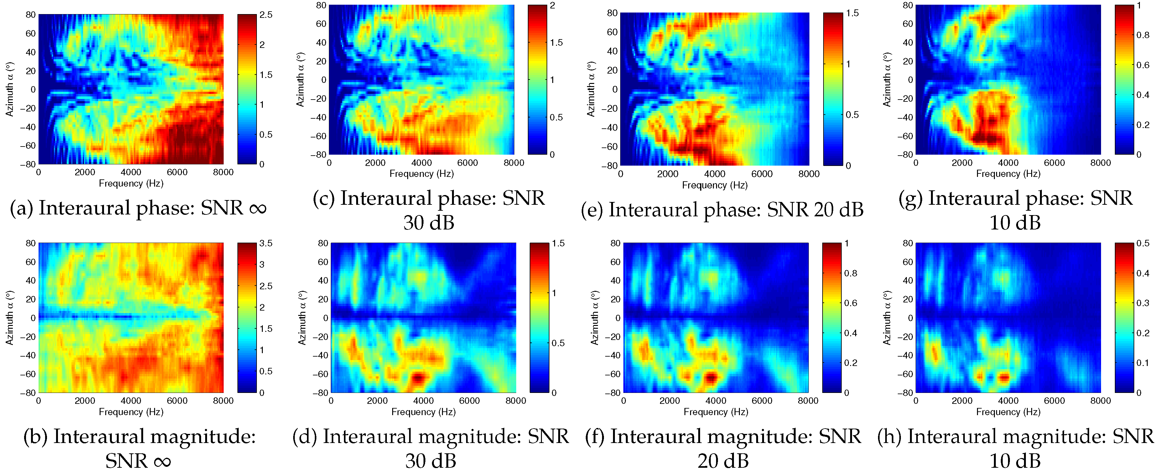
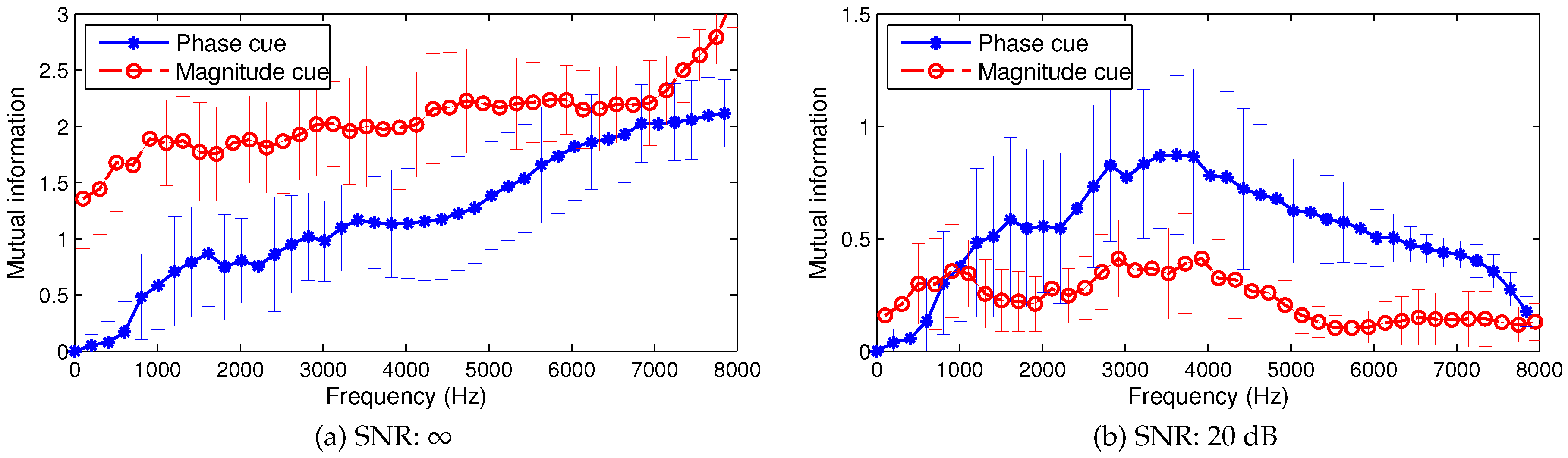
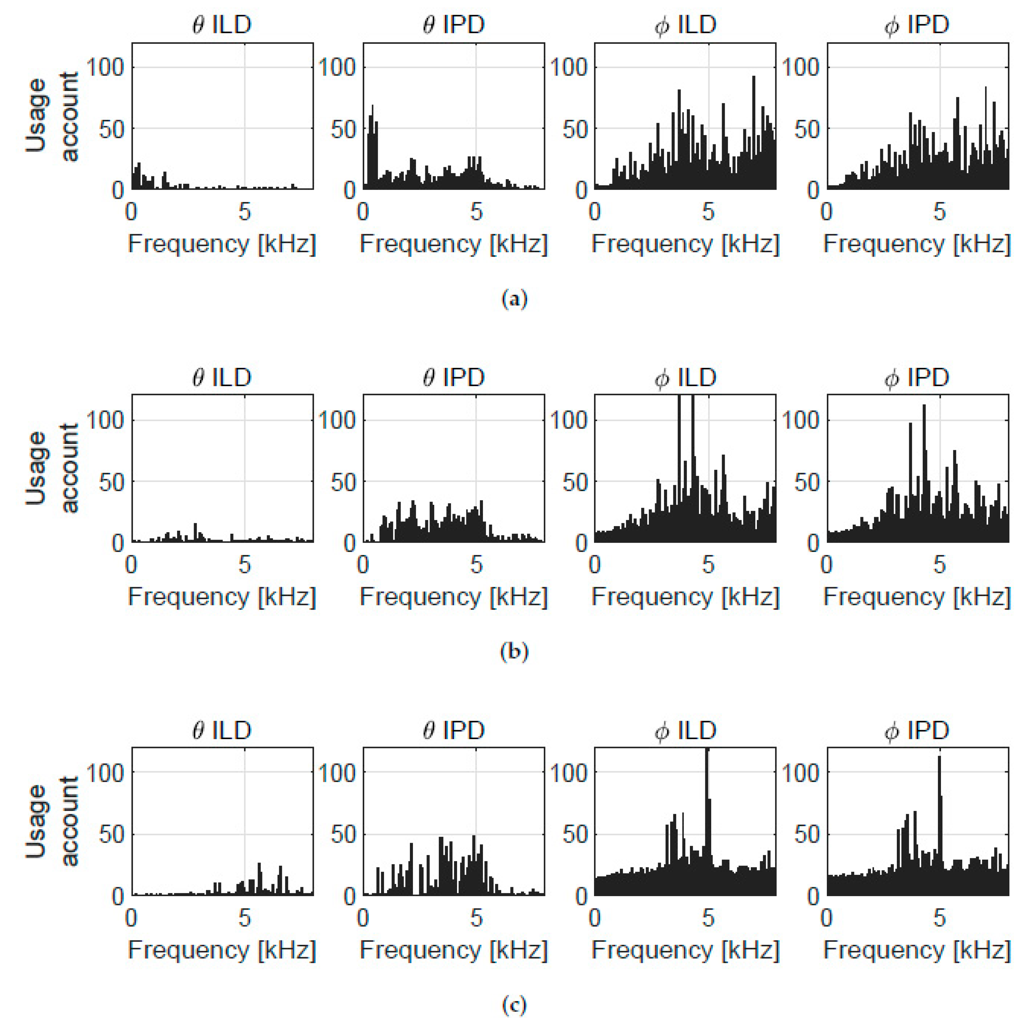
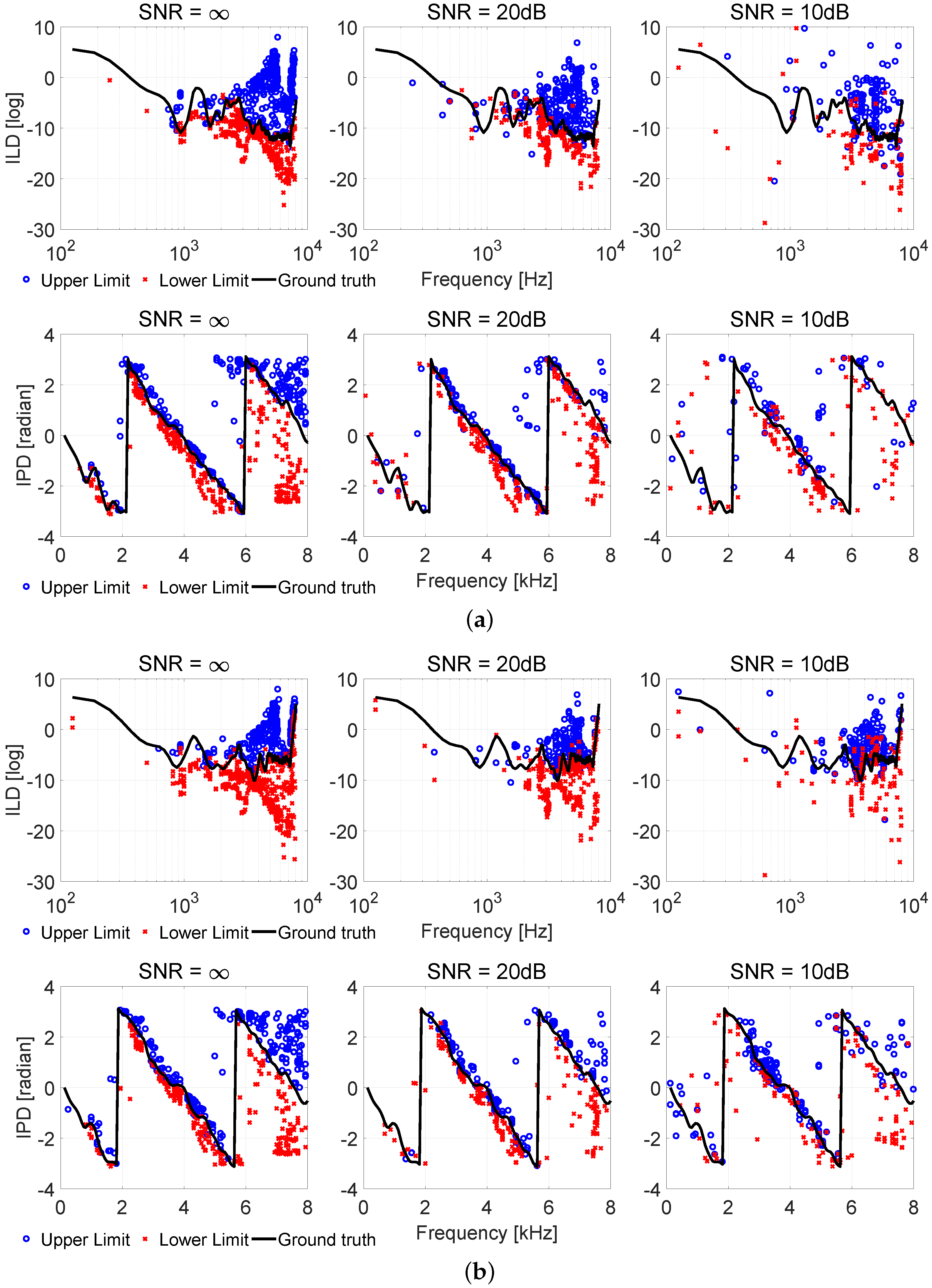
2.2. Analysis of Mutual Information in Interaural Cues

Figure 1 illustrates the variations in MI that exist between the elevation angle of the source location and the spatial cues for different azimuths and SNRs. From Figure 1a,b, it can be observed that, in high SNR scenarios, the MI in the high-frequency range becomes dominant for elevation localization. However, with the decreasing SNRs, the high-frequency cues no longer provide reliable localization information, unlike the mid-frequency spatial cues. Further, the distribution (in frequency) of the most effective cues varies with different azimuths, and illustrates both the difficulty of decoupling the localization process into separate azimuth and elevation estimation problems, as well as the challenge of localization in the median plane [24].

Further, comparing the behaviour of the two types of spatial cues, we can observe that the importance of each changes with the SNR. For example, where no or low noise is present, the interaural magnitude cues become dominant, while, in a comparably higher noise environment, the interaural phase cues show more robustness. Collectively, these observations imply that the selection of spatial cues for the creation of a feature vector for localization must be more nuanced than the simple selection of a fixed frequency range; thus, an adaptive noise-dependent feature selection and extraction process becomes a necessity for any noise-robust binaural localization system. A spatial feature learning algorithm that is aware of the MI contained in each spatial cue can satisfy this requirement, and provides superior performance to the former approach, as illustrated in the following sections.

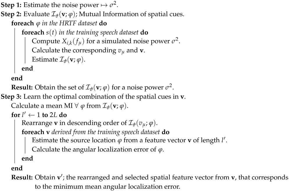
2.3. Spatial Feature Learning and Selected Feature Vector

Algorithm 1 describes the MI-based spatial feature learning mechanism used in the remainder of this work. Given an estimated noise level, such as using the method proposed in [29], the spatial feature vector $\mathbf{v}$ and its corresponding MI in (9) are computed for a set of training speech signals. Figure 2 illustrates the variation of the MI between spatial cues and elevation angle with and without noise, and indicates the changing nature of the importance of individual spatial cues. The error bar reflects the MI variation on different azimuth planes, and the mean MI obtained for the training speech dataset is used thereafter to create a rearranged spatial feature vector ${\mathbf{v}}^{\prime }$.

Algorithm 1: Spatial feature learning for robust localization

To arrive at ${\mathbf{v}}^{\prime }$, an optimal number of spatial cues to be used in the localization process $l^{\prime }$ is computed. The average angular localization error, obtained from the estimated source location $(\vartheta ,\phi )$ and its estimate $(\widehat{\vartheta },\widehat{\phi })$, is used as a metric to determine the optimal $l^{\prime }$. This results in a set of spatial feature vectors, ${\mathbf{v}}^{\prime }(\vartheta ,\phi )$, applicable to the specified noise level (in the case of some practical applications, it is also possible to pre-train the system for a set of known, approximate noise conditions). The spatial cues extracted from the received signals are rearranged similarly, and the resultant feature vector ${\widehat{\mathbf{v}}}^{\prime }$ and the ${\mathbf{v}}^{\prime }(\vartheta ,\phi )$ reference features are used to calculate vector distance for localization [25]. The localization performance will be presented in Section 6.

3. Probabilistic Localization Model and System Design

In the previous section, a feature selection approach based on averaged MI was introduced. The average MI approach provides a selection of the most dependent spectra characteristics, while the actual feature value and most related directions are not considered. In this chapter, those two feature properties are investigated and integrated with the localization mapping progress. With the proposed mapping operation, not only are the features exploited in advance, but the localization robustness will also be further improved.

Aiming at localizing the sound source in a real-world environment with presence of noise and interference, the localization problem is considered probabilistic mapping between the feature vector and source location ${\Theta }_{\mathrm{IP}}=(\vartheta ,\phi )$, which can be expressed as:

$${\widehat{\Theta }}_{\mathrm{IP}}=\underset{{\Theta }_{\mathrm{IP}}}{\arg \max }P\left({\Theta }_{\mathrm{IP}}\right|\widehat{\mathbf{v}})$$

(10)

where $P\left({\Theta }_{\mathrm{IP}}\right|{\widehat{\mathbf{v}}}_p)$ represents the probability of the sound source located at ${\Theta }_{\mathrm{IP}}$ with a given feature vector ${\widehat{\mathbf{v}}}_p$. In the interaural-polar coordinate system, the generic ITDs are the same when the sources are placed on the same sagittal plane; thus, it is more applicable to estimate the azimuth $\vartheta$ first, and then estimate the elevation $\phi$ with a given $\vartheta$. Therefore, the probability $P\left(\vartheta \right|{\widehat{\mathbf{v}}}_p)$ can be represented based on the conditional chain rule by a multiplication of two posteriors as:

$$P\left({\Theta }_{\mathrm{IP}}\right|{\widehat{\mathbf{v}}}_p)=P\left(\vartheta \right|\widehat{\mathbf{v}})P\left(\phi \right|\vartheta ,\widehat{\mathbf{v}})$$

(11)

where $P\left(\phi \right|{\widehat{\mathbf{v}}}_p)$ represents the probability of the source located at the sagittal plane, labelled by $\vartheta$, and $P\left(\phi \right|\vartheta ,{\widehat{\mathbf{v}}}_p)$ represents the probability of $\beta$ with given $\alpha$ and ${\widehat{\mathbf{v}}}_p$. Then, by substituting (11) into (10), the estimated source location ${\widehat{\Theta }}_{\mathrm{IP}}={\widehat{f}}_{{\Theta }_{\mathrm{IP}}}\left({\widehat{\mathbf{v}}}_p\right)$ can be obtained. There are two obvious advantages of adopting such localization architecture. First, in the training process, the feature characteristics caused by $\vartheta$ and $\phi$ are separated, so the localization model can be more explainable and a more accurate localization result can be achieved [21]. Second, in the testing process, the $\vartheta$ and $\phi$ can be estimated in parallel, and then high computation efficiency in contemporary parallel hardware can be achieved.

To estimate the $P\left(\alpha \right|{\widehat{\mathbf{v}}}_p)$ and $P\left(\beta \right|\alpha ,{\widehat{\mathbf{v}}}_p)$ for the real-world source localization, the estimation approaches should be able to tackle the amount of noise in the input feature vector. In the next section, the RF method is introduced to select the most important features and provide a robust estimation.

4. Feature Dependency Analysis and Assembled Data Partition Model

This section presents a posterior estimation method with adaptive feature selection approach. First, the dependency between the spatial parameters and feature characteristics is analysed, and then an assembled data partition model based on the feature dependency is adopted for the posterior estimations. During the model training process, the following notations are used in the later content: let ${\{{\mathbf{v}}^{\left(n\right)},{\mathrm{y}}^{\left(n\right)}\}}_{n=1}^N$ denote the dataset of all training data pairs, where $\mathbf{v}\in \mathcal{V}\subset {\mathbb{R}}^{2K}$ represents the interaural feature vectors in vector space $\mathcal{V}$, and ${\mathrm{y}}^{\left(n\right)}\in \{{\mathrm{y}}_1,{\mathrm{y}}_2,\dots {\mathrm{y}}_D\}$ represents the discrete spatial label. In the training dataset, either $\alpha$ or $\beta$ is discretised and labelled. Here, both labels of $\theta$ or $\phi$ are represented by the common symbol $\mathrm{y}$ for simplicity. The subscripts $n\in \{1\dots N\}$, $\mu \in \{1\dots 2K\}$ and $d\in \{1\dots D\}$, respectively, represent the training observations index, the feature vector components and the discrete label index.

4.1. Data Partition and Tree-Structured Model

The dependency analysis described in Section 2 justifies the existence of elevation-related features at full-band ILD and high-frequency IPD. To use these results and further exploit the feature characteristics, the mapping model should satisfy two essential requirements. First, the model should be able to handle both linear and non-linear associations. Second, an adaptive feature selection should be embedded in the model training progress. Therefore, to fulfil these two requirements, a recursive tree-structured data partition technique—the so-called decision tree method—is introduced. A tree is a hierarchical structure in which each internal node contains a specific feature condition. At each node, the training data are split into two sub-spaces by the splitting feature that maximizes the MI between the selected feature and the spatial labels from sub-spaces. Notably, the MI here is also known as information gain in machine learning, which is still denoted by $\mathcal{IG}$ in latter content. Finally, each node at the terminal of the tree is defined as a leaf node, which represents a subclass of spatial labels $\mathrm{y}$.

Formally, let $m\in \{1\dots M\}$ denote the splitting node index, and the subset of training data at $m\mathrm{th}$ node are defined as ${\{{\mathbf{v}}_m^{\left(n\right)},{\mathrm{y}}_m^{\left(n\right)}\}}_{n=1}^{N_m}$, where the subset of the feature vectors and the target labels are respectively represented by ${\mathcal{V}}_m\subset {\mathbb{R}}^{2K}$ and ${\mathrm{y}}_{d_m}^{\left(n\right)}\in \{{\mathrm{y}}_1,{\mathrm{y}}_2,\dots {\mathrm{y}}_{D_m}\}$. Defining ${\mathcal{V}}_{m,\mu }={\left\{v_{m,\mu }^{\left(n\right)}\right\}}_{n=1}^{N_m}$ as $\mu \mathrm{th}$ feature subset, the information gain with the binary splitting operation using the splitting value $v_{m,\mu }$ can be obtained by:

$$\begin{array}{cc}\hfill \mathcal{IG}(\mathrm{y},v_{m,\mu })=& \sum _{d=1}^D{P}_m(v_{m,\mu },{\mathrm{y}}_d)log\frac{P_m(v_{m,\mu },{\mathrm{y}}_d)}{P_m\left(v_{m,\mu }\right)P_m\left({\mathrm{y}}_d\right)}\hfill \\ & +\sum _{d=1}^D(1-P_m\left(v_{m,\mu }\right),{\mathrm{y}}_d)log\frac{1-P_m(v_{m,\mu },{\mathrm{y}}_d)}{\left(1-P_m\left(v_{m,\mu }\right)\right)P_m\left({\mathrm{y}}_d\right)}\hfill \end{array}$$

(12)

which can also be interpreted as subtraction of entropies by:

$$\mathcal{IG}(\mathrm{y},v_{m,k})=H\left(\mathrm{y}\right)-H\left(\mathrm{y}\right|v_{m,k}).$$

(13)

It is more directly perceived through (13) that the $\mathcal{IG}$ is evaluating the decreasing uncertainty of $\mathrm{y}$ after splitting by $v_{m,\mu }$.

The probability components $P_m(v_{m,\mu },{\mathrm{y}}_d)$, $P_m\left(v_{m,\mu }\right)$ and $P_m\left({\mathrm{y}}_d\right)$ are estimated by histogram-based probability estimation [28] as:

$$\begin{array}{cc}\hfill P_m(v_{m,\mu },{\mathrm{y}}_d)& =\frac{1}{N_m}\sum _{n=1}^{N_m}z(v_{m,\mu }^{\left(n\right)}\le v_{m,\mu },\mathrm{y}={\mathrm{y}}_d)\hfill \\ \hfill P_m\left(v_{m,\mu }\right)& =\frac{1}{N_m}\sum _{n=1}^{N_m}z(v_{m,\mu }^{\left(n\right)}\le v_{m,\mu })\hfill \\ \hfill P_m\left({\mathrm{y}}_d\right)& =\frac{1}{N_m}\sum _{n=1}^{N_m}z({\mathrm{y}}_{m,d}^{\left(n\right)}={\mathrm{y}}_d)\hfill \end{array}$$

(14)

where the indicator function $z(·)$ is defined as same as (9).

Depending on (12) and (14), one may split the dataset by selecting the feature index $\mu$ and its splitting value $v_{m,\mu }$, which maximizes the value of information gain as:

$${\tilde{v}}_{m,\mu }=\underset{v_{m,\mu }\in {\mathcal{V}}_m}{\arg \max }\mathcal{IG}(\mathrm{y},v_{m,k})$$

(15)

where ${\tilde{v}}_{m,\mu }$ indicates the optimized splitting value with its feature index $\mu$ at node m.

By repeating this splitting operation until some certain criteria is reached (e.g., the maximum number of nodes M), the original dataset ${\{{\mathbf{v}}^{\left(n\right)},{\mathrm{y}}^{\left(n\right)}\}}_{n=1}^N$ is partitioned into multiple subsets denoted as ${\{{\mathbf{v}}_{\lambda }^{\left(n\right)},{\mathrm{y}}_{\lambda }^{\left(n\right)}\}}_{n=1}^{N_{\lambda }}$ with subset index $\lambda$. The whole training progress can also be understood as a recursive clustering process, whereby the training data with common feature characteristics described by $v_k^m$ are clustered into the same subset $\lambda$, while the uncertainty of spatial label $\alpha$ is minimized, so that, in such a subset, the training data only share a few $\alpha$. Further, in this recursive approach, the splitting feature index k and its corresponding value $v_k^m$ are adaptively re-selected via (15) at each node, so the most spatial dependent feature characteristics are exploited to the maximum.

Then, with a test feature vector $\widehat{\mathbf{v}}$, the model will first categorise it into a subset with the splitting criteria obtained during training, and then the estimated posterior ${\widehat{P}}_{\gamma }\left({\mathrm{y}}_d\right|\widehat{\mathbf{v}})$ from a single tree $\gamma$ is given by:

$${\widehat{P}}_{\gamma }\left({\mathrm{y}}_d\right|\widehat{\mathbf{v}})=\frac{1}{N_{\lambda }}\sum _{n=1}^{N_{\lambda }}z({\mathrm{y}}^{\left(n\right)}={\mathrm{y}}_d|{\mathrm{y}}^{\left(n\right)}\in {\mathrm{y}}_{\lambda }){|}_{\widehat{\lambda }={\mathcal{C}}_{\gamma }\left(\widehat{\mathbf{v}}\right)}$$

(16)

where ${\mathcal{C}}_{\lambda }(·)$ indicates the classification approach in the tree $\gamma$ based on the splitting features, and $\widehat{\lambda }$ represents the estimated subset index. To avoid over-fitting and increase the robustness of the model, a committee of multiple single trees is constructed in the next section.

4.2. Random Forest Bagging and Unbiased Probability Estimation

A more robust posterior estimation can be obtained by an ensemble model, and the approach to assembling multiple decision trees is known as the tree bagging technique. The idea is to attain the final posterior probability estimation by averaging the probabilities from a committee of i.d.d. trees. Formally, in a forest with $\Gamma$ trees, the assembled posterior estimate is given by [28,30]:

$$\widehat{P}\left({\mathrm{y}}_d\right|\widehat{\mathbf{v}})=\frac{1}{\Gamma }\sum _{\gamma =1}^{\Gamma }{\widehat{P}}_{\gamma }\left({\mathrm{y}}_d\right|\widehat{\mathbf{v}})$$

(17)

where $\gamma \in \{1,2,\dots ,\Gamma \}$ is the index of i.d.d. trees, and the i.d.d. trees are obtained by introducing randomness into their training process. Many approaches have been proposed to randomise those training processes, and the most famous one, adopted by the RF algorithm [30], has shown its effectiveness in many applications. The independence between decision trees is achieved by introducing randomness into both the training subset and feature selection. The training datasets for each tree are obtained via bootstrap sampling, in which roughly two-thirds of the data are selected for each subset.

The averaging operation in (17) softly selects those more confident trees from the forest, and such selection is undertaken on the leaves of the trees. In a RF, each i.d.d. tree can be understood as a union of hyper-rectangles defined by the subsets on each leaf, and the boundaries of each hyper-rectangle are determined by the splitting features $v_k^m$. Although those hyper-rectangles vary with different trees, they overlap because of the similarity of feature characteristics and spatial label clustering. Thus, the operation in (17) selects the area with the maximum amount of overlaps of hyper-rectangles.

Finally, the source position estimation is given by:

$$<\widehat{\alpha },\widehat{\beta }>=\underset{<\alpha ,\beta >}{\arg \max }\widehat{P}\left(\alpha \right|{\widehat{\mathbf{v}}}_p)\widehat{P}\left(\beta \right|\alpha ,\widehat{\mathbf{v}})$$

(18)

The following content presents a detailed description of model training and parameter selection, and demonstrates an interpretation of this model.

5. Model Training and Interpretation

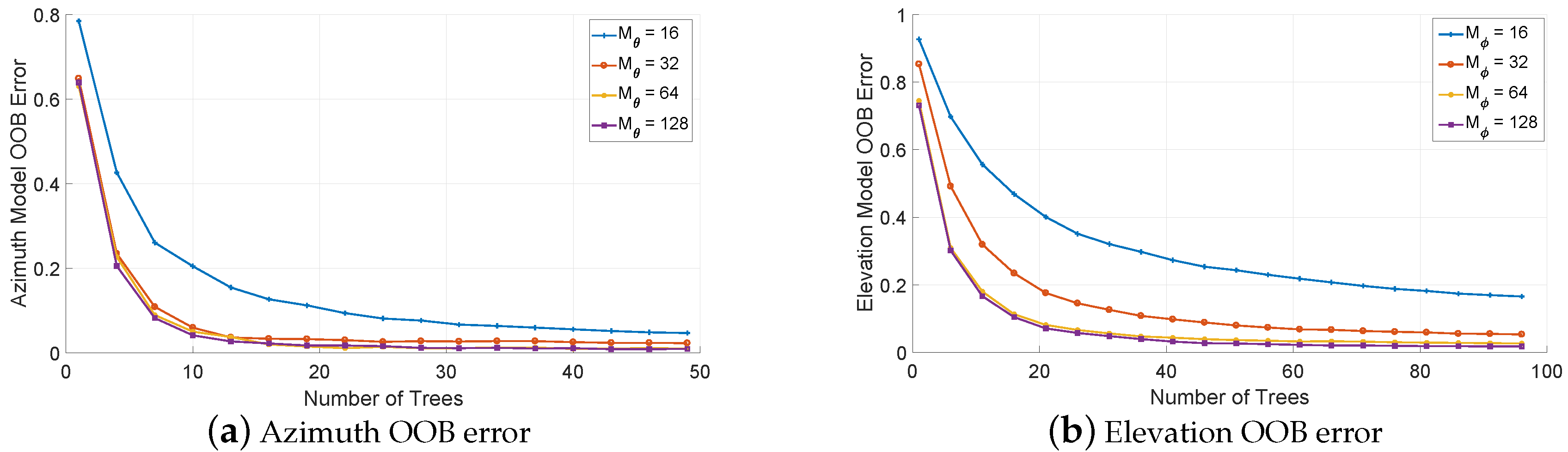
5.1. Model Training and Parameter Selection

A dataset of synthetic received signals is used for training purposes, and is generated by convolving the source signal and Head-Related Impulse Response (HRIR) in the time domain. The Gaussian noise with about 0.5 s duration is adopted as the source signal and convolved with ‘003’ subject HRIR from the CIPIC database [24], in which the HRIR were recorded at 25 sagittal azimuths and 50 elevations on each sagittal plane. The interaural features are extracted as described in Section 2.3, and we use 16 ms length Hamming window for Short-Time Fourier Transform (STFT) with 8 ms shift, so there are 256 samples with a 16 kHz sampling rate. The selection of window length is based on the assumption of application scenario as a speech source in an indoor environment, so 16 ms is corresponding to 5 m direct path, and the speech signal can be considered as stationary in such short-term. The interaural feature extracted from each frame is treated as a training sample, and 10 samples for each position are randomly selected from the dataset. Moreover, three training conditions with different SNR additive white noise are applied on the training dataset, with the aim of investigating the influence of training data quality.

In the proposed model, three parameters need to be settled during the training: the candidate feature number at each node, the splitting iteration number M and the tree number $\Gamma$. The initial value of $K^{\prime }$ can be set as the square root of the total feature numbers in $\mathbf{v}$, according to [30], and the other two parameters for the azimuth and elevation model are determined by multiple out-of-bag (OOB) data tests on different parameters combinations. Fortunately, the sampling scheme of RF provides a convenient measurement to evaluate the model using OOB error. Recall that around two-thirds of training data were selected as training data after the bootstrap sampling for each tree, so that those un-selected data could be used as testing data. The estimation error of the OOB data is defined as OOB error. Figure 3 shows the OOB errors versus $\Gamma$ of the azimuth model and elevation model with different selection of M, where the splitting iteration number of the azimuth and elevation model are defined as $M_{\theta }$ and $M_{\varphi }$, and the tree numbers are defined as ${\Gamma }_{\theta }$ and ${\Gamma }_{\varphi }$, respectively. Intuitively, M should relate to the class label number and correspond to the accuracy of the model. It can be observed from Figure 3 that small OOB error differences are obtained after a certain number of iterations—that is, $M_{\theta }=32$ and $M_{\varphi }=64$—which means the forests are fully developed for the classifications. As for the tree numbers, the OOB error tends to converge at ${\Gamma }_{\theta }=30$ for the azimuth model and ${\Gamma }_{\varphi }=80$ for the elevation model. However, since a larger tree number can increase the robustness of the model, 20 extra trees are added on both models, and the final tree numbers are settled as ${\Gamma }_{\theta }=50$ and ${\Gamma }_{\varphi }=100$.

5.2. Trained Model Interpretation

Figure 4 shows the changes in feature selection because of different training conditions, by comparing the feature usage account. Given that the features with higher information gain are more likely to be selected as splitting features at each node, the usage account of a feature in the forest describes its dependency on the position estimation. It can be observed that, in the azimuth model trained with noise-free data, the more frequently used features are clustered at frequencies under 1 kHz, which correspond to the phase delays caused by the head width. However, in the model trained by a noisy dataset, the feature usage is more evenly distributed, which indicates that the model tends to use group delays between the ears for the estimation, which is because more features are necessary to a robust estimation with noisy training data. However, an opposite phenomenon is observed in the elevation model. With the decreasing of training data SNR, the more frequently used features are clustered to the frequency range around 3 to 5 kHz. This can be ascribed to the fact that more elevation information is generally drowned by the increasing noise, which cannot provide valid localization information. Such an adaptive selection process can only benefit the model performance when the noise is relatively low, which will diversify the feature usage and tree structures. However, when the noise is too strong and the most valuable features are degraded, the tree structures are homogenised and the robustness of the model will rapidly decrease.

Figure 5 demonstrates the feature characteristics captured by the splitting values from the direction $[{30}^{\circ },{45}^{\circ }]$ and $[{30}^{\circ },{135}^{\circ }]$. In each sub-plot, each column shows the additive noise SNR for a training dataset and each row shows the type of features. Each blue circle represents a ‘left’ condition in a node from a single tree, which is also defined as the upper limit of $v_{m,k}$ in (14). Similarly, each red cross represents a ‘right’ condition in a node or the lower limit value of $v_{m,k}$. The ground truth features are plotted in black solid curves, which are obtained from pure HRTF data. Each marker, either a circle or cross, is considered a classifier to evaluate whether an extracted feature vector fits the conditions for a specific direction. By observing the distribution of markers, it again justifies that the features in frequency above 2 kHz are more valuable. The ground curves almost overlap with the dividing line between circles and crosses, which indicates that the major features have been captured by those upper and lower limits. In each row, the influence of the training condition can be compared. In the case where SNR = ∞, though the curve fits best, the markers are distributed closer, which means that the independence between trees is comparably low, which may lead to over-fitting on some features. Meanwhile, in SNR = 10 dB, the markers are more dispersed and the dividing lines are blurred because of the high noise level, which will cause loss of some details of the feature characteristics, and lead to decreasing localization accuracy.

6. Experiments With Simulated Data

6.1. 3-D Space Localization with Mutual Information–Based Feature Selection

This section presents the simulation results of 3-D space localization with MI-based feature selection. The localization performance of the proposed method is compared with the generic composite feature-based localization approach [25] and a simple correlation-based method [31].

6.1.1. Simulation Configuration

The proposed approach is used to evaluate 950 source locations, ranging from azimuth $\alpha =-{45}^{\circ }$ to ${45}^{\circ }$ in $5^{\circ }$ intervals and elevation $\beta =-{45}^{\circ }$ to $230.{625}^{\circ }$ in $5.{625}^{\circ }$ increments, for the first 10 subjects’ HRTF measurements in the CIPIC database [24]. The speech samples from the PASCAL ‘CHiME’ Speech Separation and Recognition Challenge [32] (34 males and females, each with 500 utterances sampled at 16 kHz) are used as inputs; 340 randomly selected utterances are used for the learning process, and a separate 200 utterances are used to evaluate the localization performance. The binaural signals are simulated by convolving the HRTFs of different locations with the uncorrupted speech, and introducing the independent additive white Gaussian noise with three different SNRs of 10, 20 and 30 dB.

The frequency range for the generic composite feature-based approach is selected empirically, where [0,4] kHz and [3,5] kHz are the phase and magnitude feature regions for the feature-based method, while the full-band signal is used for the correlation approach. During the comparison, the mean angular error is employed as a metric to assess the localization performance. The angular error denotes the angular distance between the estimated and actual source directions in the interaural-polar coordinate system; therefore, the estimation errors of both the azimuth and elevation ($\alpha$ and $\beta$) are implicitly included in the performance assessment.

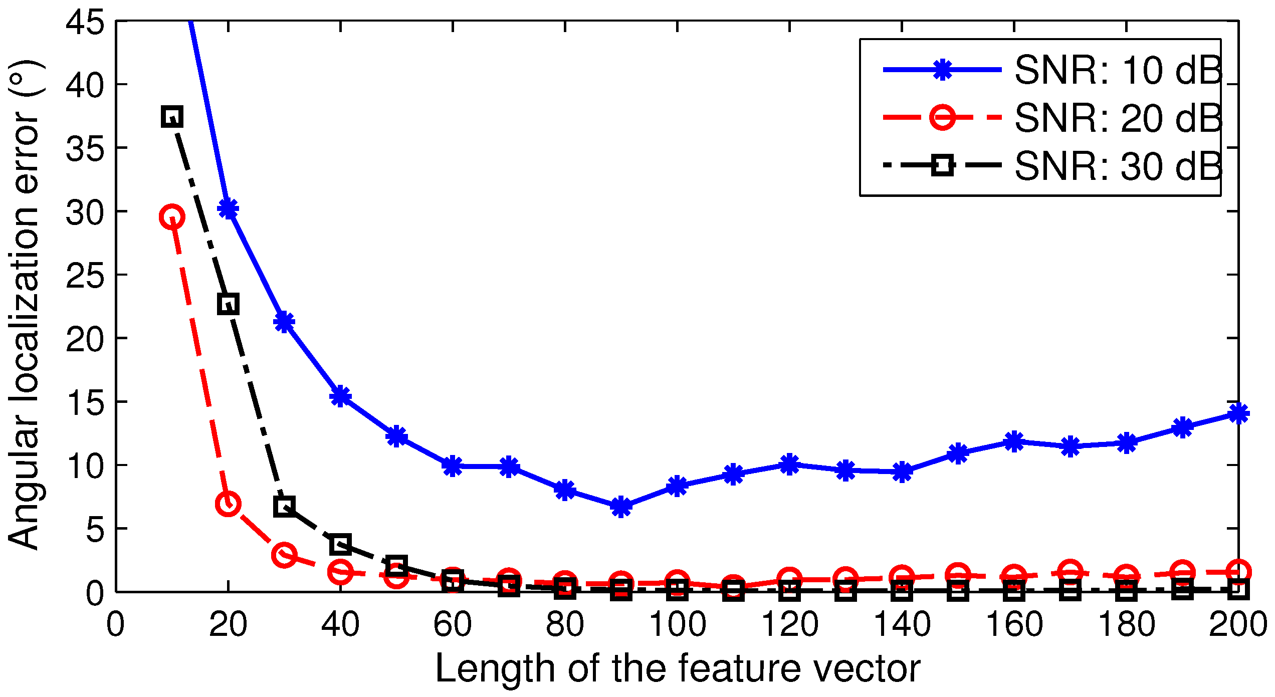
6.1.2. Performance Impact of the Feature Vector Length

From Figure 1 and Figure 2, it becomes apparent that the length of the feature vector $\tilde{\mathbf{v}}$ can directly influence the localization performance. For example, a length smaller than the optimum will result in insufficient spatial information (especially in the case of the median plane), while a greater length could result in increased ambiguity because of the effects of noise. In both cases, the mean angular localization error will be affected; thus, an optimum length for $\tilde{\mathbf{v}}$ that minimizes this error must be computed at the noise power level observed in a particular localization scenario. Hence, the training process described in Algorithm 1 is applied to a range of simulated speech inputs, and the optimum feature vector length and spatial cue combination is obtained dynamically based on their MI content.

Figure 6 illustrates the relationship between the mean angular errors and the length of the composite feature vector at different noise levels. The results are presented for three different SNRs, where the selected number of spatial cues varies from 10 to 200 in intervals of 10. The result for the 10 dB SNR case clearly illustrates the general behaviour discussed above (similar behaviour is observed at other noise levels as well), indicating an optimum feature vector length of approximately 90 elements. Note that the angular localization error for the 30 dB scenario is larger than that for the 20 dB scenario when the feature vector length is less than 60. This suggests that a short feature vector may lead to unstable localization performance; thus, a minimum length of the feature vector should be guaranteed.

6.1.3. Localization Performance

The performance of the proposed method is presented and compared with two other approaches in

Table 1. 3-D space localization performance comparison.

Localization Approach	Mean Angular Localization Error
	10 dB	20 dB	30 dB
Proposed learning	5.63${}^{\circ }$	0.89${}^{\circ }$	0.14${}^{\circ }$
Composite feature [25]	24.30${}^{\circ }$	5.11${}^{\circ }$	0.85${}^{\circ }$
Cross-Correlation [31]	67.65${}^{\circ }$	58.55${}^{\circ }$	51.58${}^{\circ }$

. Here, the received binaural inputs are obtained from 90 uniformly sampled source locations of the 950 locations in the HRTF dataset, and the resulting localization error is averaged across multiple untrained speech inputs and source locations. The results indicate a significant improvement in performance over the generic composite feature-based localization approach in [25], especially in the low SNR configurations. It was notable that the improvement predominantly stemmed from a reduction in front-to-back confusion. This suggests that the approach overcomes the lack of spectral cues located beyond the mid- to high-frequency ranges [33] that are less robust to the effects of noise. In general, the results suggest that the MI-based feature learning and rearrangement of the spatial cues in the feature vector can both improve the localization performance and overcome the negative effect of the dynamic truncation of the feature vector to achieve greater robustness to noise.

6.2. 3-D Space Localization with Probabilistic Model

To evaluate the accuracy and robustness of the proposed method, localization tests proceed with multiple testing conditions, and the localization results are compared with the state-of-the-art PPAM method [17]. In the last part of this section, performance in different reverberant environments is also compared and presented.

6.2.1. Performance Measurements and Simulation Configuration

The received signals are generated by convolving the simulated Binaural Room Impulse Response (BRIR) and speech utterances. The speech utterances are obtained from the PASCAL ‘CHiME’ Speech Separation and Recognition Challenge database [32], which includes 34 speakers and every speaker has 500 utterances. Each testing speech utterance has around 1 s duration.

The BRIRs used in the testing are generated with CIPIC HRTF subject ‘003’ and the Roomsim MATLAB program [34] based on the image method in four empty ‘shoebox’ rooms. A rectangular room with room sizes 5 m × 5 m × 3 m is created in the simulation. The subject head is fixed at (2.5, 2.5, 1.2) m and the sound source is positioned around the subject with the same position scheme as used in the CIPIC database, so there are 1250 source positions (25 azimuths × 50 elevations) in total during the tests. The distance between the sound source and the center of the head is fixed as 1.5 m so that the acoustical environment can be considered a far-field environment. The strengths of reflections are manipulated by the absorption coefficients $\beta$ on the walls. In the additive noise test, four sets of data are generated and tested with different SNRs. The absorption coefficients are set as $\beta =1$, so no reflections present and the interference is entirely caused by noise. As for the reverberation test, the absorption coefficients are tuned from 0.8 to 0.2, and the corresponding $T_{60}$ varies from 100 to 500 ms approximately.

The localization accuracy is evaluated by the correct rate of localization. An estimation is considered correct if the difference between the estimated sound direction and ground truth source position is below a certain tolerance threshold. To objectively demonstrate the 3-D position differences between the ground truth source position and the estimated direction, the angular error defined by the absolute angular difference between two directional vectors in a Cartesian coordinate system is calculated as:

$$ϵ=arccos\frac{{\mathbf{d}}_{<\alpha ,\beta >}·{\widehat{\mathbf{d}}}_{<\widehat{\alpha },\widehat{\beta }>}}{|{\mathbf{d}}_{<\alpha ,\beta >}\left|\right|{\widehat{\mathbf{d}}}_{<\widehat{\alpha },\widehat{\beta }>}|}$$

(19)

where ${\mathbf{d}}_{<\alpha ,\beta >}$ and ${\widehat{\mathbf{d}}}_{<\widehat{\alpha },\widehat{\beta }>}$ are the ground truth source direction vector and the estimation direction vector in Cartesian coordinate system, respectively. The azimuth and elevation correct rate in the interaural-polar system are also presented.

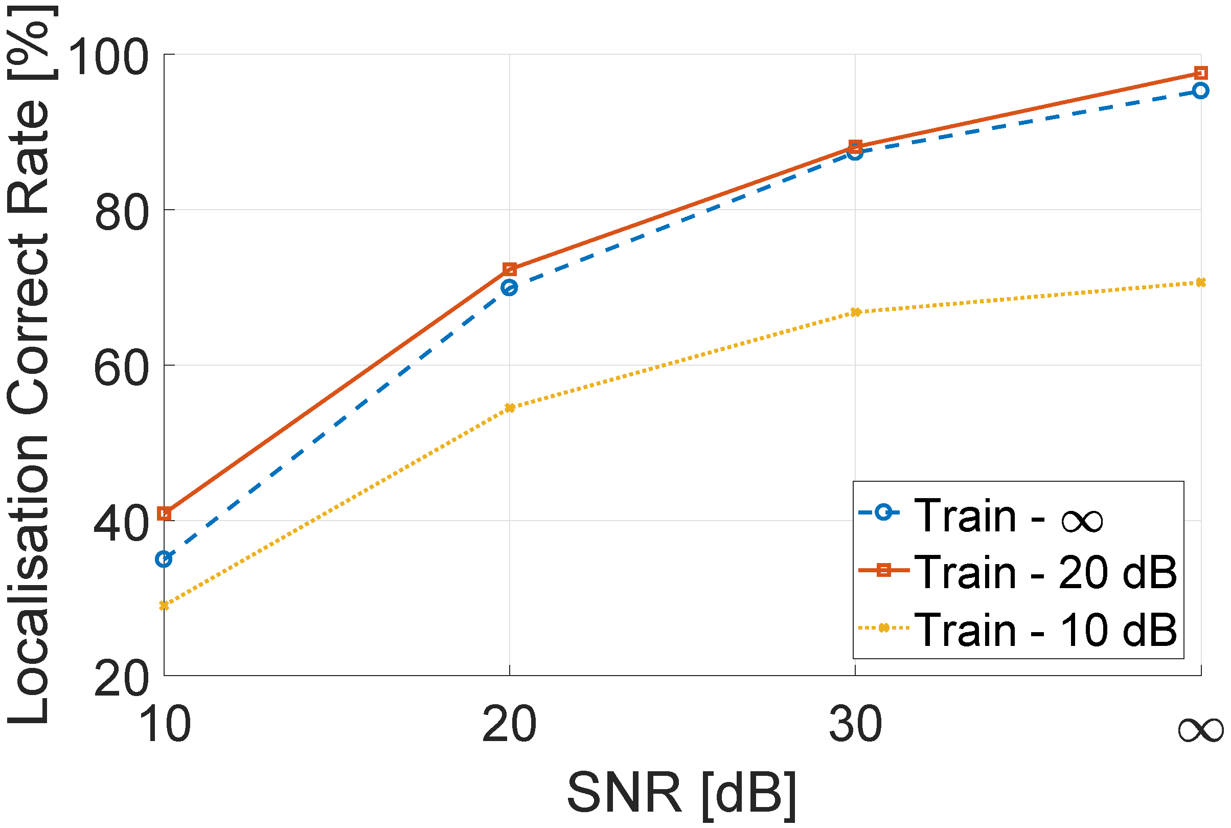
6.2.2. Localization Performance with Different Training Environment

As discussed in Section 5.2, different training conditions also affect the quality of the model, which leads to different localization performance. In this section, the localization performances with different training conditions are presented and compared in Figure 7.

In general, the localization accuracy for all models decreases with increasing noise level. As predicted in Section 5.2, the model trained with moderate noise conditions performs best, and slightly outperforms the one trained with no noise data. This is because the additive zero-mean Gaussian noise increases the variance of the training data, which introduces diversity in the splitting values for all features and forces trees to select the features that can still provide valuable information under interference. However, the localization result of the model trained in a strong noise environment entirely degrades because the model cannot capture the details of feature characteristics from noisy data, as demonstrated in the third column of Figure 5. According to this comparison result, in the following simulations, moderate noise data are used as training data for both the proposed and reference method for comparison.

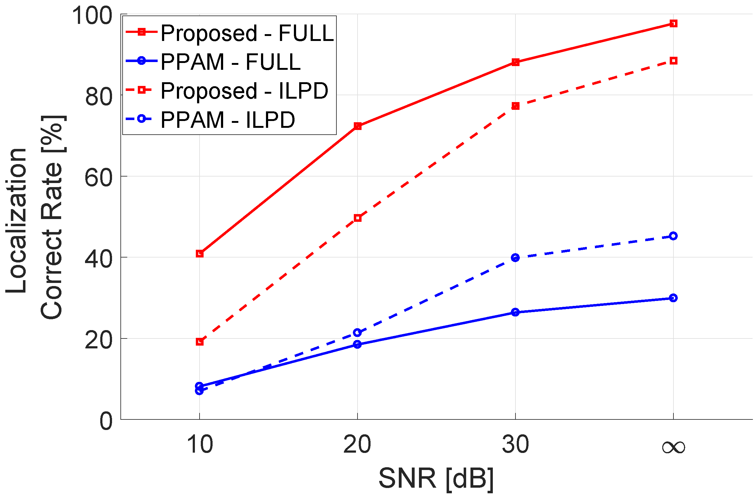
6.2.3. Localization Performance with Additive Noise

A localization accuracy comparison with the presence of additive noise is shown in Figure 8. In general, the proposed method outperforms the state-of-the-art method with both feature vector types. It can be concluded that the RF algorithm in the proposed method is capable of constructing a finer mapping between the feature characteristics and source locations, and this mapping shows robustness to additive noise. Further, through comparing the performance with different feature vectors yet the same localization method, it can be observed that better performance is obtained by using a full ILD and IPD spectrum in the proposed method, while a more accurate result is achieved by using the full-spectrum ILD and low-frequency IPD (ILPD) vector in PPAM. This different feature preference proves that the proposed method successfully exploits the non-linear cues in the high-frequency IPD spectrum, and such cues will contribute to a more accurate result.

A more detailed comparison between the azimuth and elevation estimation is provided in

Table 2. Azimuth and elevation estimation accuracy comparison in noisy environment.

(a) Azimuth Accuracy Comparison
SNR	No Noise		30 dB		20 dB		10 dB
Tolerance	≤2.5${}^{\circ }$	≤5${}^{\circ }$	≤2.5${}^{\circ }$	≤5${}^{\circ }$	≤2.5${}^{\circ }$	≤5${}^{\circ }$	≤2.5${}^{\circ }$	≤5${}^{\circ }$
Proposed - FULL	$99.44\%$	$100.0\%$	$98.88\%$	$100.0\%$	$97.20\%$	$99.60\%$	$94.40\%$	$97.92\%$
PPAM - FULL	$79.92\%$	$91.12\%$	$79.52\%$	$90.72\%$	$75.36\%$	$87.6\%$	$61.36\%$	73.84%
Proposed - ILPD	$95.68\%$	$97.12\%$	$87.68\%$	$90.56\%$	$78.96\%$	$86.00\%$	$68.64\%$	$79.44\%$
PPAM - ILPD	$89.28\%$	$96.96\%$	$86.64\%$	$95.68\%$	$73.84\%$	$89.44\%$	$55.04\%$	73.84%
(b) Elevation Accuracy Comparison
SNR	No Noise		30 dB		20 dB		10 dB
Tolerance	≤2.5${}^{\circ }$	≤6${}^{\circ }$	≤2.5${}^{\circ }$	≤6${}^{\circ }$	≤2.5${}^{\circ }$	≤6${}^{\circ }$	≤2.5${}^{\circ }$	≤6${}^{\circ }$
Proposed - FULL	$96.08\%$	$99.52\%$	$89.60\%$	$96.72\%$	$72.64\%$	$83.84\%$	$37.04\%$	$51.20\%$
PPAM - FULL	$28.08\%$	$47.12\%$	$24.48\%$	$44.80\%$	$19.52\%$	$34.64\%$	$9.20\%$	$17.20\%$
Proposed - ILPD	$94.40\%$	$97.12\%$	$76.96\%$	$84.00\%$	$48.72\%$	$58.88\%$	$17.76\%$	$27.04\%$
PPAM - ILPD	$44.72\%$	$71.92\%$	$40.72\%$	$63.28\%$	$24.26\%$	$41.44\%$	$9.84\%$	$18.24\%$

. Again, better estimation results can be obtained from the proposed method in general. In Table 2a, the proposed method using full ILD/IPD spectrum vectors achieves the best result and maintains a high estimation accuracy in a severe condition. Meanwhile, the result from the proposed method using ILPD features has comparably good performance in a noise-free environment, yet degrades rapidly with decreased SNR. There are two causes of this phenomenon. First, a longer feature vector increases the diversity of available feature candidates at each splitting node; hence, the independence between decision trees increases and the forest becomes more robust. Second, the RF algorithm extracts the spatial cues at high-frequency IPD spectrum (e.g., the group delay) and those cues contribute to the estimation even in a noisy environment. In Table 2b, although the elevation estimation accuracy from all methods decreases obviously with increased noise level, the proposed method can provide a precise estimation in the high SNR scenario, compared with the results from PPAM, which indicates that elevation-related feature characteristics extracted by the RF algorithm are non-linear and more sensitive to interference.

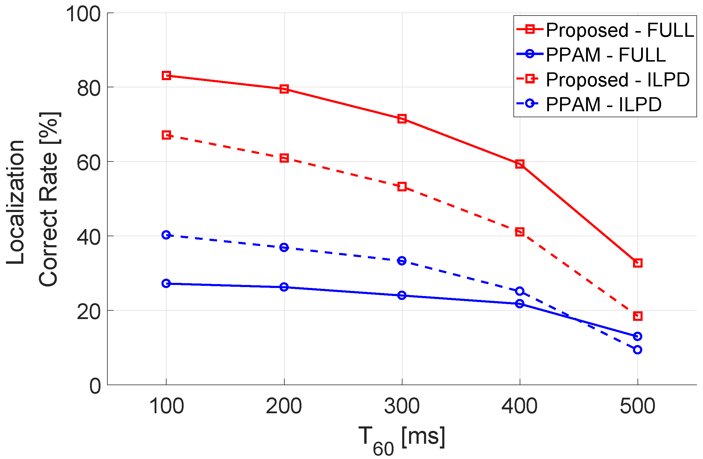
6.2.4. Localization Performance with Reverberations

To localize the sound source in a reverberant environment, the proposed method introduces the Direct Path Relative Transfer Function (DP-RTF) estimation method as a pre-processing front-end in the system. In the DP-RTF extraction, because the reverberation condition is assumed unknown, the CTF length $Q_k$ is settled as 0.25 s and remains unchanged in all simulations. Figure 9 shows the compared localization performances with multiple reverberation configurations. Although all methods are degraded in more severe environments, the proposed methods have more accurate localization results for both feature vector types, and the best performance is achieved by using full length vectors. It can be concluded that the high-IPD features still contain source direction information and, with an appropriate application, can contribute to the source position estimation in a reverberant environment.

Similar to the previous subsection, the azimuth and elevation estimations are compared separately in

Table 3. Azimuth and elevation estimation accuracy comparison in reverberate environment.

(a) Azimuth Accuracy Comparison
${\mathit{T}}_{60}$	200 ms		300 ms		400 ms		500 ms
Tolerance	≤2.5${}^{\circ }$	≤5${}^{\circ }$	≤2.5${}^{\circ }$	≤5${}^{\circ }$	≤2.5${}^{\circ }$	≤5${}^{\circ }$	≤2.5${}^{\circ }$	≤5${}^{\circ }$
Proposed - FULL	$94.32\%$	$97.92\%$	$91.44\%$	$96.72\%$	$89.44\%$	$95.76\%$	$78.88\%$	$89.12\%$
PPAM - FULL	$81.04\%$	$90.64\%$	$79.84\%$	$90.32\%$	$77.84\%$	$88.88\%$	$66.35\%$	$85.76\%$
Proposed - ILPD	$74.24\%$	$84.96\%$	$72.08\%$	$83.28\%$	$66.32\%$	$80.4\%$	$53.04\%$	$74.88\%$
PPAM - ILPD	$86.72\%$	$96.88\%$	$96.40\%$	$77.20\%$	$77.2\%$	$94.96\%$	$58.00\%$	83.92%
(b) Elevation Accuracy Comparison
${\mathit{T}}_{\mathbf{60}}$	200 ms		300 ms		400 ms		500 ms
Tolerance	≤2.5${}^{\circ }$	≤6${}^{\circ }$	≤2.5${}^{\circ }$	≤6${}^{\circ }$	≤2.5${}^{\circ }$	≤6${}^{\circ }$	≤2.5${}^{\circ }$	≤6${}^{\circ }$
Proposed - FULL	$75.84\%$	$89.04\%$	$68.48\%$	$82.72\%$	$55.52\%$	$72.56\%$	$42.64\%$	$62.80\%$
PPAM - FULL	$26.16\%$	$96.88\%$	$23.92\%$	$40.00\%$	$21.12\%$	$35.52\%$	$14.12\%$	24.80%
Proposed - ILPD	$61.92\%$	$42.64\%$	$53.76\%$	$70.32\%$	$42.08\%$	$61.04\%$	$22.48\%$	$40.24\%$
PPAM - ILPD	$37.36\%$	$61.60\%$	$34.08\%$	$55.44\%$	$28.96\%$	$46.80\%$	$15.68\%$	$28.00\%$

. In the azimuth comparison, the state-of-the-art method has better performance when using the ILPD feature vector, which indicates that the high-IPD features are crucial to the proposed method to tackle the interference caused by reverberation. As for the elevation localization, a considerably better elevation performance can be obtained by using the proposed methods with both vector types, which proves that mapping of elevation exploited by the RF algorithm can work well against the reverberate interference.

7. Experiment in Laboratory Environment

The proposed methods can localize a sound source accurately and robustly based on the simulation result. However, testing the proposed methods in practical environments remains necessary because the simulated data are generated based on a mathematical model with several assumptions, which might be difficult to achieve in a practical environment. Therefore, in this section, the proposed localization methods are tested with data recorded in a real indoor environment with the existence of reverberation and background noise.

The experimental evaluation of the localization performance is conducted in an enclosed laboratory at the Australian National University. A GRAS KEMAR manikin Type 45BA human-like simulator is used to collect the binaural testing data, which is performed by playing a source signal via loudspeakers fixed at different directional positions. Two Type 40AG polarized pressure microphones are placed at the entrance of the ear canal of the dummy head. To test the robustness and practicality of the proposed method, the testing dataset is collected in a real laboratory environment, while the training data are synthesized as described in the previous chapters based on the open HRTF database (i.e., CIPIC database) [24]. Hence, the testing environment is completely unfamiliar to the localization model, and no prior knowledge about the room acoustical characteristic is learned during the training process.

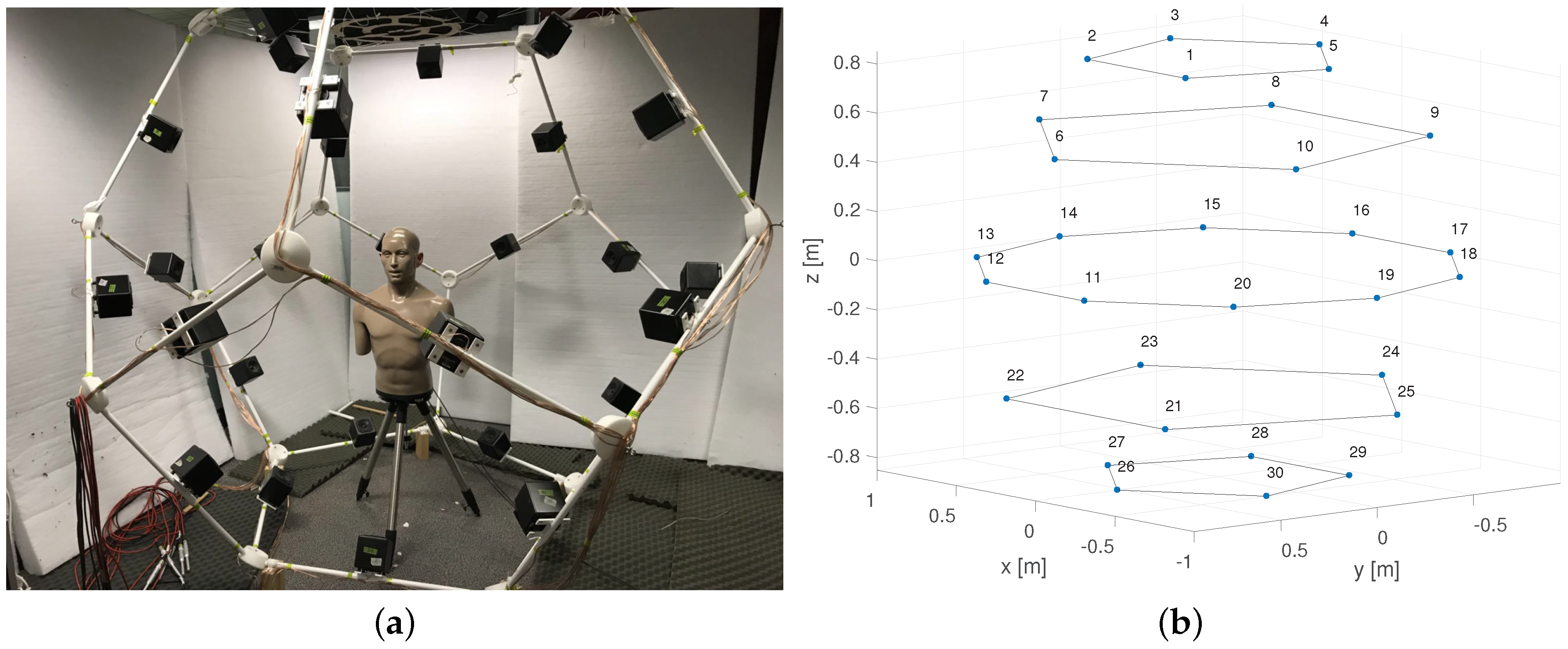
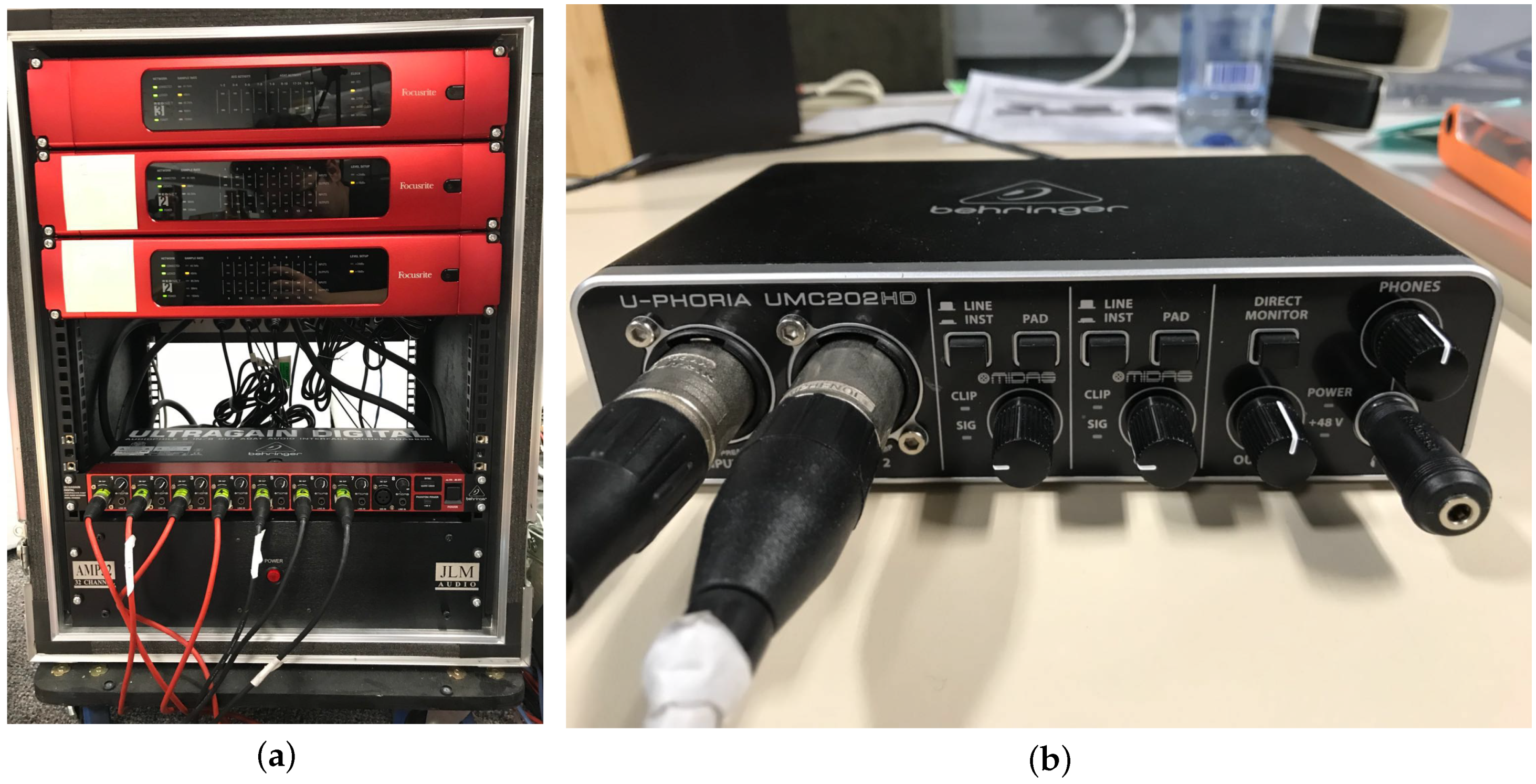
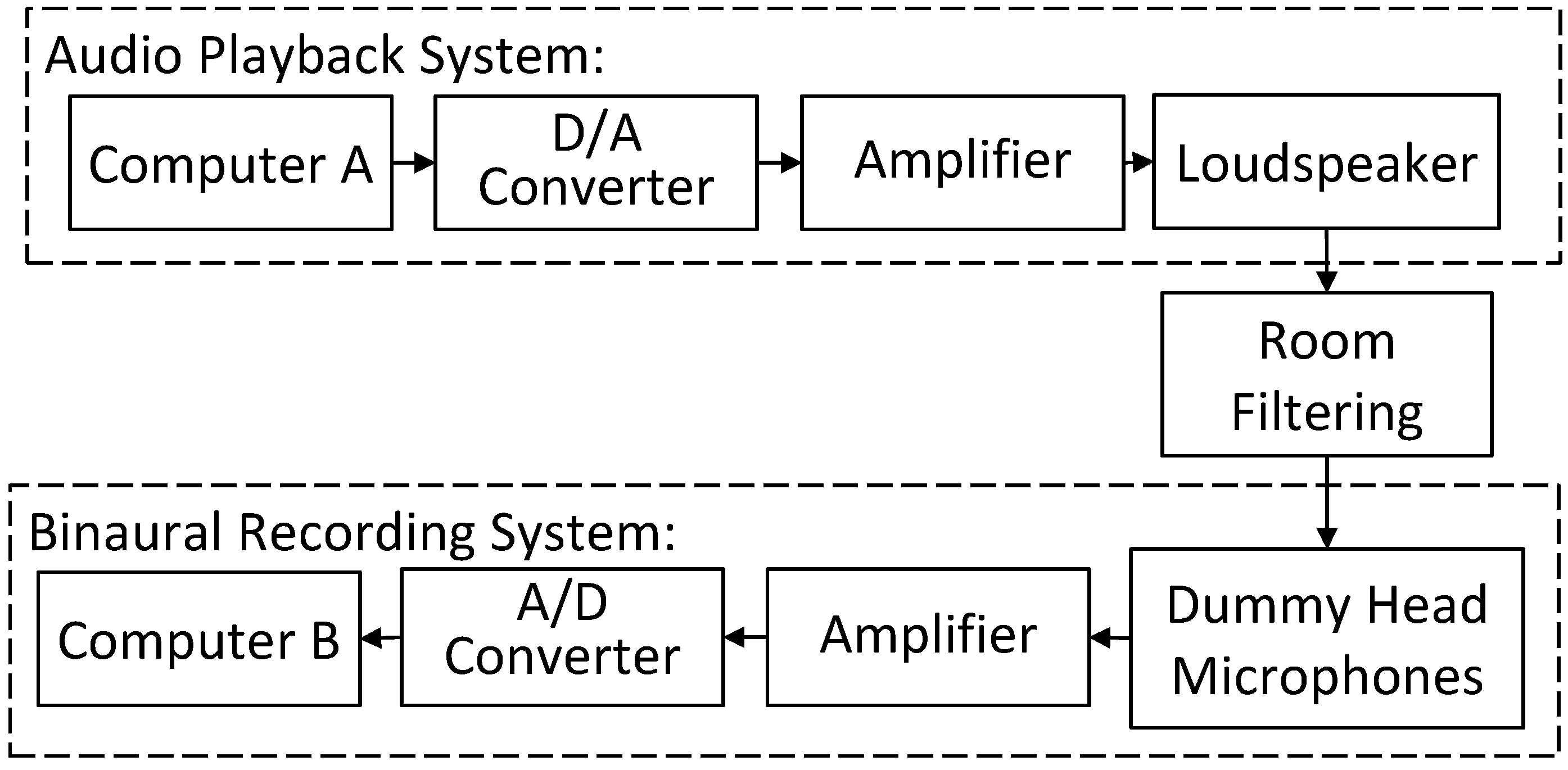
7.1. Experiment Facility and Room Configurations

The experiment system can be generally separated into two independent subsystems: the audio playback system and the binaural signal recording system. The general structure and connection relationship of the systems is shown in Figure 10, and the setup of the experiment is shown in Figure 11a. In this system, the source signal is played by the audio playback system via spatially placed loudspeakers. Then, the emitted signal then propagates through the space and is captured by the recording system. Notably, The recorded signals are pre-processed and delivered to another computer for the localization. The later content includes the more detailed configurations of the two systems.

In the audio playback system, 30 loudspeakers are placed on a regular dodecahedron. The loudspeakers are fixed on the middle of the edges and face to the center of the dodecahedron, as shown in Figure 11a. Figure 11b demonstrates the ground truth loudspeaker array placement positions and their corresponding labels in the Cartesian coordinate system. All loudspeakers are driven by the Dante audio network system, as shown in Figure 12a, which is controlled by a computer. As for the recording system, the signals are captured by two Type 40AG polarized pressure microphones planted in the ear canals of the dummy head. The captured signals are then converted via the U-PHORIA UMC202HD audio interface and transferred to another computer via a USB connection.

In the experiment, we first switch on the recording system, and then play the source signal with one of 30 loudspeakers with selected positions. The signals captured by the recording system are converted and delivered to the localization systems, and the estimated source location can be obtained. In such a system setup, the generation of directional audio signal and the process of localization are physically isolated, so the performance of the localization entirely relies on the recorded signals, and no prior knowledge about the source signal and environmental acoustic configurations can be obtained by the localization system. Therefore, the robustness and flexibility of the proposed methods can be examined.

7.2. Testing Positions and Microphone Data Pre-Processing

As aforementioned, the source signal is played by an array of 30 loudspeakers, so the ground truth source positions are identical to the locations of the loudspeakers. Figure 11b and

Table 4. To performance of the passive model. The ground truth loudspeaker locations are represented in ${\Theta }_{\mathrm{IP}}$.

Loudspeaker No.	True Azimuth	True Elevation	Estimated Azimuth	Estimated Elevation	Estimated Error
1	$-18.{00}^{\circ }$	63.44${}^{\circ }$	$-22.{00}^{\circ }$	81.68${}^{\circ }$	35.25${}^{\circ }$
2	18.00${}^{\circ }$	63.44${}^{\circ }$	20.00${}^{\circ }$	67.50${}^{\circ }$	4.33${}^{\circ }$
3	30.00${}^{\circ }$	100.82${}^{\circ }$	30.00${}^{\circ }$	71.43${}^{\circ }$	31.53${}^{\circ }$
4	0.00${}^{\circ }$	121.72${}^{\circ }$	$-5.{00}^{\circ }$	123.75${}^{\circ }$	2.03${}^{\circ }$
5	$-30.{00}^{\circ }$	100.82${}^{\circ }$	$-30.{00}^{\circ }$	84.38${}^{\circ }$	14.04${}^{\circ }$
6	0.00${}^{\circ }$	31.72${}^{\circ }$	0.00${}^{\circ }$	33.75${}^{\circ }$	2.03${}^{\circ }$
7	54.00${}^{\circ }$	63.44${}^{\circ }$	55.00${}^{\circ }$	60.19${}^{\circ }$	3.56${}^{\circ }$
8	30.00${}^{\circ }$	142.62${}^{\circ }$	30.00${}^{\circ }$	140.63${}^{\circ }$	1.73${}^{\circ }$
9	$-30.{00}^{\circ }$	142.62${}^{\circ }$	$-30.{00}^{\circ }$	135.56${}^{\circ }$	6.11${}^{\circ }$
10	$-54.{00}^{\circ }$	63.44${}^{\circ }$	$-55.{00}^{\circ }$	59.06${}^{\circ }$	2.82${}^{\circ }$
11	$-18.{00}^{\circ }$	0.00${}^{\circ }$	$-20.{00}^{\circ }$	0.00${}^{\circ }$	2.00${}^{\circ }$
12	18.00${}^{\circ }$	0.00${}^{\circ }$	19.50${}^{\circ }$	10.69${}^{\circ }$	11.88${}^{\circ }$
13	54.00${}^{\circ }$	0.00${}^{\circ }$	55.00${}^{\circ }$	0.00${}^{\circ }$	1.48${}^{\circ }$
14	90.00${}^{\circ }$	0.00${}^{\circ }$	80.00${}^{\circ }$	$-39.{94}^{\circ }$	10.00${}^{\circ }$
15	54.00${}^{\circ }$	180.00${}^{\circ }$	55.00${}^{\circ }$	194.06${}^{\circ }$	9.61${}^{\circ }$
16	18.00${}^{\circ }$	180.00${}^{\circ }$	20.00${}^{\circ }$	177.75${}^{\circ }$	3.47${}^{\circ }$
17	$-18.{00}^{\circ }$	180.00${}^{\circ }$	$-18.{00}^{\circ }$	157.50${}^{\circ }$	24.36${}^{\circ }$
18	$-54.{00}^{\circ }$	180.00${}^{\circ }$	$-55.{00}^{\circ }$	182.81${}^{\circ }$	2.21${}^{\circ }$
19	$-90.{00}^{\circ }$	0.00${}^{\circ }$	$-80.{00}^{\circ }$	$-39.{94}^{\circ }$	10.00${}^{\circ }$
20	$-54.{00}^{\circ }$	0.00${}^{\circ }$	$-55.{00}^{\circ }$	1.69${}^{\circ }$	2.69${}^{\circ }$
21	$-30.{00}^{\circ }$	$-37.{38}^{\circ }$	$-30.{00}^{\circ }$	$-38.{81}^{\circ }$	1.87${}^{\circ }$
22	30.00${}^{\circ }$	$-37.{38}^{\circ }$	30.00${}^{\circ }$	$-33.{75}^{\circ }$	3.14${}^{\circ }$
23 ${}^{*}$	54.00${}^{\circ }$	243.43${}^{\circ }$	55.00${}^{\circ }$	168.75${}^{\circ }$	41.26${}^{\circ }$
24	0.00${}^{\circ }$	211.74${}^{\circ }$	$-5.{00}^{\circ }$	219.38${}^{\circ }$	9.14${}^{\circ }$
25 ${}^{*}$	$-54.{00}^{\circ }$	243.43${}^{\circ }$	$-55.{00}^{\circ }$	101.25${}^{\circ }$	66.65${}^{\circ }$
26 ${}^{*}$	0.00${}^{\circ }$	$-58.{29}^{\circ }$	0.00${}^{\circ }$	$-33.{75}^{\circ }$	24.54${}^{\circ }$
27 ${}^{*}$	30.00${}^{\circ }$	$-79.{19}^{\circ }$	30.00${}^{\circ }$	73.13${}^{\circ }$	114.47${}^{\circ }$
28 ${}^{*}$	18.00${}^{\circ }$	243.43${}^{\circ }$	20.00${}^{\circ }$	196.88${}^{\circ }$	43.93${}^{\circ }$
29 ${}^{*}$	$-18.{00}^{\circ }$	243.43${}^{\circ }$	$-20.{00}^{\circ }$	157.50${}^{\circ }$	80.27${}^{\circ }$
30 ${}^{*}$	$-30.{00}^{\circ }$	$-79.{19}^{\circ }$	$-30.{00}^{\circ }$	$-33.{75}^{\circ }$	39.08${}^{\circ }$

${}^{*}$ indicates the indexes of out-of-range speakers.

illustrate the ground truth positions of loudspeakers represented in the interaural-polar coordinate system with the label indices. The testing loudspeaker positions are not presented in the training positions. Thus, a correct estimation should be the nearest location label to the ground truth. Notably, there are six loudspeakers placed beyond the training region, which are marked by ${}^{*}$ in Table 4. Those loudspeakers are muted during the following tests, since the localization of these speakers is meaningless.

One issue that must be noted is that the impulses of the two microphone channels cannot be identical in the real world, and small differences lead to inaccuracy in localization. Therefore, in the binaural recording system, the raw signals captured by the binaural microphones are equalized before passing to the localization model, which aims at minimizing the amplitude difference between channels. The equalization is performed by multiplying a generic compen coefficient ${\zeta }_l$ on the left-ear channel, and this coefficient is pre-measured in two steps. First, one 2 s white noise signal is played as the source signal by each loudspeaker, and the captured signals are notated as $x_{1,l,k}(t,\Theta )$ and $x_{1,r,k}(t,\Theta )$. Second, the connection of two channels is switched and the same source signals are played by each speaker again. The signals captured by the switched channel are notated as $x_{2,l,k}(t,\Theta )$ and $x_{2,r,k}(t,\Theta )$. Ideally, if the two channels are identical, we would have $x_{1,l,k}(t,\Theta )=x_{2,r,k}(t,\Theta )$ and $x_{1,r,k}(t,\Theta )=x_{2,l,k}(t,\Theta )$. Therefore, the estimated left-ear compensation coefficient ${\widehat{\zeta }}_l$ can be estimated by averaging all frames and positions as:

$${\widehat{\zeta }}_l=\sum _{k,\Theta }\left[\frac{x_{2,r,k}(t,\Theta )}{x_{1,l,k}(t,\Theta )}+\frac{x_{1,r,k}(t,\Theta )}{x_{2,l,k}(t,\Theta )}\right]$$

(20)

and hence, the binaural signals for To are calibrated by,

$$\begin{array}{cc}\hfill x_l(t,\Theta )& ={\widehat{\zeta }}_l·x_{1,l,k}(t,\Theta )\hfill \\ \hfill x_l(r,\Theta )& =x_{1,r,k}(t,\Theta )\hfill \end{array}$$

(21)

Given that the calibration is applied on the left channel for all source positions in the time domain, it is spatial and frequency independent, and does not introduce external information to estimate the sound source position.

7.3. Experiment Result

The localization performance of the probabilistic model is demonstrated in Table 4. The localization tests are repeated 10 times, and, in each test, the random selected speech utterances (around 1 to 2 s per utterance) are played as the source signal through the first 22 speakers. The results justify that the model can effectively localize the source positions. The azimuth localization is very accurate, since the model returns the nearest azimuth class to the ground truth position. Although the accuracy of elevation localization is degraded compared with the simulation results in the previous chapters, the absolute angular error remains around 10 degrees, which corresponds to around 17 cm differences with a 1 m source distance. Several factors may cause the decreasing of localization accuracy. One obvious cause is the difference of HRTF between the CIPIC database and the used dummy head. Those differences could result from assembling the dummy head in practice, which would affect the features in a high-frequency region. This issue could be resolved by replacing the training data with measured HRTFs of the subject being used. In addition, the reflections from objects in the laboratory may interfere with the localization, since there are no de-reverberation operations during testing. Notably, the localization error of those out-of-range speakers that marked by ${}^{*}$ is comparably larger to the other positions, because the labels of those out-of-range positions are not exist in the training dataset. However, if we carefully look into those localization results, the estimated azimuths of their sagittal planes are correct, and the results are suffer from the up-down confusion not front-back confusion. The up-down confusion indicates that the proposed model pinpoints the positions who share the most similar features with those unknown out-of range positions. Furthermore, these results also justify that the proposed model can use the other positions’ features to help distinguish the front and back for the unfamiliar positions, like the blocking effect of the external ears.

8. Conclusions

We have proposed a novel elevation localization model for binaural localization based on the RF algorithm. The algorithm operates on the interaural features—such as ILD and IPD—in the spectral domain. During the training process, the RF algorithm successfully selected the most reliable feature of a spectrum by using information gain, and constructed the elevation-dependent mappings simultaneously based on its selections for each sagittal plane. In the testing, the multi-tree structure showed robustness to additive noise and flexibility to an unfamiliar acoustical environment. Further, a hierarchical localization system was also proposed for 3-D space localization, which achieved outstanding localization performance in the simulation. The proposed method is also tested in a real laboratory environment, and the result justifies the effectness of the model.

References

1. Xie, B. Head-Related Transfer Function and Virtual Auditory Display; J. Ross Publishing: Plantation, FL, USA, 2013. [Google Scholar]
2. Gan, W.S.; Peksi, S.; He, J.; Ranjan, R.; Hai, N.D.; Chaudhary, N.K. Personalized HRTF Measurement and 3D Audio Rendering for AR/VR Headsets. In Proceedings of the Audio Engineering Society 142nd International Convention Committee Announced, Berlin, Germany, 20–23 May 2017. [Google Scholar]
3. Hai, N.D.; Chaudhary, N.K.; Peksi, S.; Ranjan, R.; He, J.; Gan, W. Fast HRFT measurement system with unconstrained head movements for 3D audio in virtual and augmented reality applications. In Proceedings of the 2017 IEEE International Conference on Acoustics, Speech and Signal Processing (ICASSP), New Orleans, LA, USA, 5–9 March 2017; pp. 6576–6577. [Google Scholar]
4. Sunder, K.; Gan, W.S. Individualization of Head-Related Transfer Functions in the Median Plane using Frontal Projection Headphones. J. Audio Eng. Soc. 2016, 64, 1026–1041. [Google Scholar] [CrossRef]
5. Reijniers, J.; Vanderelst, D.; Jin, C.; Carlile, S.; Peremans, H. An ideal-observer model of human sound localization. Biol. Cybern. 2014, 108, 169–181. [Google Scholar] [CrossRef] [PubMed]
6. Pereira, F.; Martens, W.L. Psychophysical Validation of Binaurally Processed Sound Superimposed upon Environmental Sound via an Unobstructed Pinna and an Open-Ear-Canal Earspeaker. In Proceedings of the Audio Engineering Society Conference: 2018 AES International Conference on Spatial Reproduction—Aesthetics and Science, Tokyo, Japan, 7–9 August 2018. [Google Scholar]
7. Gamper, H.; Tervo, S.; Lokki, T. Head Orientation Tracking Using Binaural Headset Microphones. In Proceedings of the Audio Engineering Society Convention 131, New York, NY, USA, 20–23 October 2011. [Google Scholar]
8. Braasch, J.; Martens, W.L.; Woszczyk, W. Modeling auditory localization in the low-frequency range. J. Acoust. Soc. Am. 2005, 117, 2391. [Google Scholar] [CrossRef]
9. Li, D.; Levinson, S.E. A Bayes-rule based hierarchical system for binaural sound source localization. In Proceedings of the IEEE International Conference on Acoustics, Speech and Signal Processing (ICASSP), Hong Kong, China, 6–10 April 2003; Volume 5, pp. 521–524. [Google Scholar]
10. Raspaud, M.; Viste, H.; Evangelista, G. Binaural Source Localization by Joint Estimation of ILD and ITD. IEEE Trans. Audio Speech Lang. Process. 2010, 18, 68–77. [Google Scholar] [CrossRef]
11. Woodruff, J.; Wang, D. Binaural Localization of Multiple Sources in Reverberant and Noisy Environments. IEEE Trans. Audio Speech Lang. Process. 2012, 20, 1503–1512. [Google Scholar] [CrossRef]
12. Duda, R.O. Elevation dependence of the interaural transfer function. In Binaural and Spatial Hearing in Real and Virtual Environments; Psychology Press: New York, NY, USA, 1997; pp. 49–75. [Google Scholar]
13. Keyrouz, F. Advanced Binaural Sound Localization in 3-D for Humanoid Robots. IEEE Trans. Instrum. Meas. 2014, 63, 2098–2107. [Google Scholar] [CrossRef]
14. Keyrouz, F.; Diepold, K. An enhanced binaural 3D sound localization algorithm. In Proceedings of the 2006 IEEE International Symposium on Signal Processing and Information Technology, Vancouver, BC, Canada, 27–30 August 2006; pp. 663–665. [Google Scholar]
15. Zhang, J.; Liu, H. Robust Acoustic Localization Via Time-Delay Compensation and Interaural Matching Filter. IEEE Trans. Signal Process. 2015, 63, 4771–4783. [Google Scholar] [CrossRef]
16. Liu, H.; Zhang, J.; Fu, Z. A new hierarchical binaural sound source localization method based on Interaural Matching Filter. In Proceedings of the IEEE International Conference on Robotics and Automation, Hong Kong, China, 31 May–7 June 2014; pp. 1598–1605. [Google Scholar]
17. Deleforge, A.; Forbes, F. Acoustic space learning for sound-source separation and localization on binaural manifolds. Int. J. Neural Syst. 2015, 25. [Google Scholar] [CrossRef] [PubMed]
18. Deleforge, A.; Horaud, R. 2D sound-source localization on the binaural manifold. In Proceedings of the IEEE International Workshop on Machine Learning for Signal Processing, Santander, Spain, 23–26 September 2012; pp. 1–6. [Google Scholar]
19. Weng, J.; Guentchev, K.Y. Three-dimensional sound localization from a compact non-coplanar array of microphones using tree-based learning. J. Acoust. Soc. Am. 2001, 110, 310–323. [Google Scholar] [CrossRef] [PubMed]
20. Algazi, V.R.; Avendano, C.; Duba, R.O. Elevation localization and head-related transfer function analysis at low frequencies. J. Acoust. Soc. Am. 2001, 109, 1110–1122. [Google Scholar] [CrossRef] [PubMed]
21. Li, X.; Girin, L.; Horaud, R.; Gannot, S. Estimation of the Direct-Path Relative Transfer Function for Supervised Sound-Source Localization. IEEE Trans. Audio Speech Lang. Process. 2016, 24, 2171–2186. [Google Scholar] [CrossRef] [Green Version]
22. Parisi, R.; Camoes, F.; Scarpiniti, M.; Uncini, A. Cepstrum prefiltering for binaural source localization in reverberant environments. IEEE Signal Process. Lett. 2012, 19, 99–102. [Google Scholar] [CrossRef]
23. Westermann, A.; Buchholz, J.M.; Dau, T. Binaural dereverberation based on interaural coherence histograms. J. Acoust. Soc. Am. 2013, 133, 2767–2777. [Google Scholar] [CrossRef] [PubMed]
24. Algazi, V.R.; Duda, R.O.; Thompson, D.M.; Avendano, C. The CIPIC HRTF database. In Proceedings of the IEEE ASSP Workshop on Applications of Signal Processing to Audio and Acoustics (WASPAA), New Platz, NY, USA, 24 October 2001; pp. 99–102. [Google Scholar]
25. Wu, X.; Talagala, D.S.; Zhang, W.; Abhayapala, T.D. Binaural localization of speech sources in 3-D using a composite feature vector of the HRTF. In Proceedings of the 2015 IEEE International Conference on Acoustics, Speech and Signal Processing (ICASSP), Brisbane, QLD, Australia, 19–24 April 2015; pp. 2654–2658. [Google Scholar]
26. Hanchuan, P.; Fuhui, L.; Chris, D. Feature Selection Based on Mutual Information: criteria of Max-Dependency, Max-Relevance, and Min-Redundancy. IEEE Trans. Pattern Anal. Mach. Intell. 2005, 27, 1226–1238. [Google Scholar] [CrossRef] [PubMed]
27. Vinh, L.T.; Lee, S.; Part, Y.T.; Auriol, B. A novel feature selection mehtod based on normalized mutual information. Springer Appl. Intell. 2012, 37, 100–120. [Google Scholar] [CrossRef]
28. Fan, W.; Greengrass, E.; McCloskey, J.; Yu, P.S.; Drammey, K. Effective estimation of posterior probabilities: explaining the accuracy of randomized decision tree approaches. In Proceedings of the IEEE International Conference on Data Mining (ICDM’05), Houston, TX, USA, 27–30 November 2005; p. 8. [Google Scholar]
29. Kamkar-Parsi, A.; Bouchard, M. Improved Noise Power Spectrum Density Estimation for Binaural Hearing Aids Operating in a Diffuse Noise Field Environment. IEEE Trans. Audio Speech Lang. Process. 2009, 17, 521–533. [Google Scholar] [CrossRef]
30. Breiman, L. Random Forests. Mach. Learn. 2001, 45, 5–32. [Google Scholar] [CrossRef] [Green Version]
31. Keyrouz, F.; Naous, Y.; Diepold, K. A new method for binaural 3-D localization based on HRTFs. In Proceedings of the IEEE International Conference on Acoustics, Speech and Signal Processing (ICASSP), Toulouse, France, 14–19 May 2006; Volume 5, pp. 341–344. [Google Scholar]
32. Barker, J.; Vincent, E.; Ma, N.; Christensen, H.; Green, P. The PASCAL CHiME speech separation and recognition challenge. Comput. Speech Lang. 2013, 27, 621–633. [Google Scholar] [CrossRef] [Green Version]
33. Raykar, V.C.; Duraiswami, R.; Yegnanarayana, B. Extracting the frequencies of the pinna spectral notches in measured head related impulse responses. J. Acoust. Soc. Am 2005, 118, 364–374. [Google Scholar] [CrossRef] [PubMed]
34. Campbell, R.D.; Palomki, K.J.; Brown, G. A MATLAB Simulation of “Shoebox” Room Acoustics for Use in Research and Teaching. Comput. Inf. Syst. 2005, 9, 48–51. [Google Scholar]
Figure 1. Mutual Information between the spatial cues and the elevation for a range of azimuths, frequencies and noise conditions.
Applsci 09 02682 g001
Figure 2. MI variation in spatial cues with respect to SNR.
Applsci 09 02682 g002
Figure 3. OOB errors.
Applsci 09 02682 g003
Figure 4. Feature Usage Accounts for training condition (a) SNR = ; (b) SNR = 20 dB and (c) SNR = 10 dB. The first two columns shows the feature usage for azimuth model and the last two columns shows the average feature usage for elevation model.
Applsci 09 02682 g004
Figure 5. (a) Split feature learning for θ = 30 and ϕ = 45 ; (b) Split feature learning for θ = 30 and ϕ = 135 . Split feature value comparison between (a) θ = 30 , ϕ = 45 and (b) θ = 30 , ϕ = 135 .
Applsci 09 02682 g005
Figure 6. Localization error with respect to feature vector length.
Applsci 09 02682 g006
Figure 7. Comparing the localization accuracy with different training conditions. The angular error tolerance is 2 . 5 .
Applsci 09 02682 g007
Figure 8. Comparing the localization accuracy between proposed and PPAM methods using different feature vector types. The angular error tolerance is 2 . 5 .
Applsci 09 02682 g008
Figure 9. Comparing the localization accuracy between proposed method and PPAM with different T 60 . The angular error tolerance is 2 . 5 .
Applsci 09 02682 g009
Figure 10. The experiment outline: The audio playback system and binaural recording system.
Applsci 09 02682 g010
Figure 11. The hardware setup and the loudspeaker positions. (a) The loudspeakers are positioned on the middle of edges of a dodecahedron frame, and the dummy head simulator with two microphones are placed in the center of the speaker arrays; (b) The ground truth position of sound sources and their corresponding labels.
Applsci 09 02682 g011
Figure 12. System hardware. (a) Dante audio network system; (b) U-PHORIA UMC202HD audio interface.
Applsci 09 02682 g012