Improving Lossless Image Compression with Contextual Memory

1. Introduction

Why is compression a difficult problem? In general, when it comes to predicting something, you need to understand the process behind the result. This requires the acquisition of knowledge about the environment and the potential dynamics. For example, if you know the English language, it will be rather easy to predict the letters missing from a truncated sentence. Predicting the value of the pixels in an image requires a deep understanding of what is represented in the image. The predictor needs to create an internal representation of segments that correspond to features of the image, like shapes, patterns, textures, borders, and then make a guess based on which part of the segmented image it is currently in.

An important application of image compression is in the field of medical imaging. Whether the images come from radiography, magnetic resonance imaging, ultrasonography, or by other methods, the number of acquired images is growing, which makes it increasingly necessary to use advanced compression methods. There are two important operations that require improvement: the storage of images, be it for long or short term (archiving), and the transmission of images via networks. When it comes to quality, lossy methods need to keep the quality of the image high to prevent mispronounced diagnostics. There may be cases where medical law is involved and the legislation would state that a copy of the medical images should be long term stored in lossless mode to allow diagnostic reconsideration in case of legal proceedings.

In this paper, we describe the state-of-the-art image compression method called PAQ8PX and introduce a new algorithm for online automated learning. We tailored the implementation for our proposed method by integrating it with PAQ8PX, which resulted in an improved 8 bpp grayscale model. We tested our implementation and obtained improvements on four datasets belonging to three benchmarks.

2. Related Work

Since compression is a difficult problem, the techniques used come from many branches of algorithmics. We provide a review of some of the algorithms that appeared in the literature in recent years and some of the algorithms that use a similar contextual method as ours.

Wavelet compression involves decorrelating the neighboring pixel values by convoluting them with a basis function and then entropy encoding the resulting coefficients. The Burrows–Wheeler transform involves applying a reversible sorting algorithm to the data, making it compressible using simple operations. Since these methods remove the contextual correlation in the data stream, the data compression falls into the category of non-contextual methods. There is ongoing research in the area of non-contextual methods applied for two-dimensional or three-dimensional images.

Lossless wavelet compression was improved in [1] by introducing a new family of update-then-predict integer lifting wavelets. In [2], the authors extended the Burrows–Wheeler transform to two dimensions. The bi-level Burrows–Wheeler compression algorithm applies the well-known block sorting algorithm on the rows of the image and then on the columns, for an improved homogeneity in the 2D space. It then uses a modified kernel move-to-front for the 2D subspace before the entropy coding stage.

A mixture of lossless and lossy wavelet-based color image compression has been described in [3], where the region of interest based on the saliency of the image is taken into account when sending the image progressively through the communication network. It was applied for wildlife photography where the images are sent through a limited bandwidth channel. The Region of Interest (ROI) is extracted using a convolutional neural network to create a mask. Two wavelet encoding types are then used: for the lossless part SPIHT coding, for the lossy one EZW coding.

Deep learning for residual error prediction has been described in [4]. Here, a residual-error predictive convolutional neural network (REP-CNN) is introduced with the scope of refining the prediction of the LOCO-I and CALIC predictors. In total, three REP-CNN are trained, one for direct prediction and two for predicting the residuals of the aforementioned predictors. The big disadvantage of such a method is that, in order for a decoder to work, the entire trained neural network needs to be sent along with the compressed representation.

Contextual methods are still the basis for both lossless and lossy image compression. There is a lot of diversity in the literature about the choice of context and how it is used. An example of a lossy image compression applied for medical ultrasound images relies on contextual vector quantization, as shown in [5]. In this algorithm, a separation method based on region growing distinguishes a region of interest in the image starting from a seed point. Different vector sizes are chosen for background and the contextual ROI. The regions are then encoded with high and low compression ratios respectively, and, then, are merged in a final result.

Another lossy image compression for medical imaging [6] relies on the contextual prediction of the quantized and the normalized sub-band coefficients after a discrete wavelet transform was applied.

Extending the prediction by partial matching for two dimensions for lossless compression of indexed raster images has been presented in [7]. Context models for sparse order lengths are created and stored in an AVL-tree structure. A parallelization of the coding algorithm is presented by splitting the image into independent blocks and compressing them individually.

Context-based predictor blending (CBPB) for lossless compression of color images is described in [8], which is an extension of the algorithm CBPB [9], where the image is interpreted as an interleaved sequence generated by multiple sources so that non-stationary signals are better predicted. The blending prediction weights are selected based on the texture of the surrounding pixels and a Pearson correlation coefficient is computed for adjusting these weights. The final prediction also takes into account a template matching prediction. The CBPB algorithm was also ported to parallel execution via a CUDA implementation [10].

Vanilc is a lossless image compression framework described in [11] for 8 bpp, multichannel color images, and 16 bpp medical 3D volumes. The main contribution of the paper is a pixel probability distribution predictor based on a weighted least squares approach that uses a weighting function that generalizes some of the proposed contextual schemes in the literature and provides good results when it comes to the non-stationarities in the image while having only a few tuning parameters.

A lossless image compression algorithm is described in [12]. It is based on multi-resolution compression for progressive transmission. It improves on prior work from [13], where the image is decomposed into a pyramidal data structure and an edge adaptive hierarchical interpolation is applied for coding and progressive transmission. The prediction accuracy is improved here by using context-conditioned adaptive error modeling and by passing the estimates through an error remapping function. In this way, it improves both the final bitrate and the visual quality of the reconstructed images at intermediate stages.

Another lossless medical imaging compression algorithm using geometry-adaptive partitioning and least square-based prediction is described in [14]. Because of the similarities of the images obtained from the same imaging method, a prior segmentation via geometry adaptive partitioning and quadtree partitioning of the image allows a good selection of a least squares optimized predictor for sections of the image.

For lossless compression of 3D medical images, an extension of the minimum rate predictors from 2D to 3D has been developed in [15]. Here, 3D-shaped predictors were introduced to benefit from the volumetric redundancy, and, then, volume-based optimizations are applied, and hybrid 3D block splitting and classification is done. The algorithm was also extended from 8 bpp images to 16 bpp images because they provide better diagnostic quality.

Lossless compression of multi-temporal hyperspectral images can also exploit the temporal correlations besides the spatial and spectral ones. In [16], the fast lossless predictor, a variation of the least means square applied to the causal context [17], has been extended to 4D to incorporate the temporal aspect in the prediction. The residuals are computed as the difference between the prediction and the current pixel and are then encoded using the fast Golomb-Rice coding.

3. PAQ8PX Algorithm for Lossless Image Compression in Detail

3.1. Introduction

PAQ is a series of experimental lossless data compression software aiming at the best compression ratio for a wide range of file types without a focus on using few computing resources or keeping backward version compatibility. It was started by Matt Mahoney and later developed by more than 20 developers in different branches of compression. PAQ8PX is a branch of PAQ started by Jan Ondrus in 2009 and that has recently adopted the best image compression models in the series with the help of Márcio Pais. In short, we refer to version 167 of PAQ8PX.

A detailed description of the software in its current phase is not available in the literature. The reason may be the everchanging filetype specific models and the amount of version branching this software receives, from simplified models for fast compression to platform-specific optimization tests and the generalization of the algorithms used. However, a description of the PAQ series of compressors from the perspective of machine learning is available at [18].

The description of the overall compression algorithm and the techniques used can be found in [19] and [20]. The PAQ8PX version has a development thread that can be found at [21]. The source code is written in the C++ programming language and is contained in only one file with more than 12000 lines of code. The logic was not broken into different files in order to make it easier to compile to any platform. The big downside of this is that it makes the code very difficult to read. Another thing that makes the code difficult to develop is that numerous optimization techniques were inserted along the code, which can slow down the understanding of what is going to execute and when.

3.2. General Aspects

Compressing a file goes through four main stages: preprocessing, model prediction, context mixing, and probability refining. An optional pre-training phase can be activated via command line parameters. The pipeline for image compression has been described schematically in Figure 1.

The preprocessing phase is also split into three parts. At first, it searches through the file to be compressed for known stream types. Based on these types, different models are activated for the second stage of compressing. For example, it searches for image (1 bpp, 4 bpp, 8 bpp, 8 bpp grayscale, 24 bpp, 32 bpp, png 8 bpp, png grayscale 8 bpp, png 24 bpp, png 32 bpp), jpeg, gif, text, audio (8 and 16-bit mono and stereo), exe, base64, zlib streams, file containers, and others. After this stage, an optional transform phase is applied for certain stream types such as text, where an end of line transform can be applied, or EXE, where certain instructions are replaced with others. The transform phase is then applied in reverse and if the result matches the original stream, the transform is kept.

In the case of images, the preprocessing phase extracts the file header, which is compressed separately, and the byte stream containing the pixel values of the image. The width and the bit depth of the image are extracted from the header and the width is passed on to the image model selected by bit depth.

The model prediction and context mixing phase happen consecutively. Probabilities of individual bits from the input stream are predicted by many specialized models. All the probabilities are combined into one probability via the context mixing algorithm. The output probability is refined using a network of adaptive probability maps. The final prediction is used to encode the bit from the stream using a binary arithmetic coder. The algorithm is symmetrical, meaning that both the coder and the decoder do the same operations ending up with the same final probability. The decoder uses the probability to decode the bit from the compressed stream.

3.3. Modeling

The term model is used with double meaning throughout the compressor. At first, it is used to denote the unit of the algorithm that outputs a probability that will participate in the mixing phase. One can interpret this as an “elementary” model. The second meaning is the collection of units that are modeling a given type of data. The output of such models is, evidently, a collection of probabilities. Example models are TextModel (for language-specific language stemming and word modeling), MatchModel (for repeatable long matches of data), RecordModel (for data structured in records), SparseModel, JpegModel (for specific jpeg data), WavModel, ExeModel, DmcForest (a collection of dynamic Markov coding models), XmlModel, PpmModel (various order prediction by partial matching), ImageModels (for different bit depth image data), and many more. One or more of this type of model is selected according to the input stream type and compression parameters.

It is outside of the scope of this paper to explain models unrelated to image compression. These can be further detailed in a general compression paper.

3.4. Image Compression

In the case of image streams, the match model can be optionally activated and can bypass the image model if there is a long match found. But our focus will be set on the 8 bpp image model. The output of this model contains predictions for four types of input streams: 8 bpp indexed color or grayscale and 8 bpp png indexed or grayscale. If the stream is png, a part of the filtering scheme used is undone in order to obtain the true pixel value.

Depending on the type of image, different correlations can be expected and, thus, exploited by specific modeling. Before describing the specific contexts, we should describe which types of operations are possible with the contexts. Three major types of models can be identified: direct, indirect, and least squares modeling. All of these models expect byte level context values (as data coming from a file comes in byte chunks) and can output direct probabilities, stretched probabilities, or both. The context mixing stage expects probabilities in the logistic domain (stretched probabilities) and different operations are applied to probabilities to fit or skew them into this domain.

3.4.1. Direct Modeling

Direct modeling is implemented with the use of stationary context maps. This type of map takes as input a context value and outputs a weighted stretched probability and a weighted probability centered around zero (skewing). It is implemented using a direct lookup table where each entry stores a probability (which is then stretched and skewed) and a hit counter. On the update phase, an error is computed as the difference between the stored probability and the value of the bit. The error is weighted with a value dependent on the hit counter. Fewer hits on the context value indicate a more rapid update rate. This is implemented via a lookup table containing the values of an inverse linear function of the hit count.

For each context that requires direct modeling, a new map must be created. This protects the contexts from colliding with each other.

3.4.2. Indirect Modeling

Unlike direct modeling, which updates the probability based on the last probability predicted, indirect modeling tries to learn the answer based on a similar sequence from the past.

Indirect modeling is implemented with the use of indirect context maps, which use two-step mapping. An optional run context map is also included, which is used for modeling runs of bits.

The first mapping is between a context value and a bit history called state. The state is modeled as an 8-bit value with the following meaning: A zero value means the context value was never seen before. States from 1 to 30 map all the possible 4-bit histories. The rest of the states represent bit counts of zero and one or an approximation of the ratio between zeroes and ones if the number of previously seen bits exceeds a count of 16. The states are used as indexes in a state table which contains transitions to the next state depending on the value of the next bit. The states were empirically chosen to try to model non-stationarity and different state maps were proposed in other compression programs [22].

The states are kept in a hash map implemented as a table with 64-byte entries to fit in a cache line. The entries contain checksums for the context value to prevent collisions and up to seven state values. Since the map expects byte data, at bit 0, 2, and 5, the bucket for a context value is recomputed via a dispersion function. The seven state values can hold information about no bits known (one value), one bit known (two values), and two bits known (four values). At bit zero, only three states are needed and, as an optimization, the next four bytes implement a run map that predicts the last byte seen in the same context value, logarithmically weighted by the length of the run. The hash map implements a “least frequently used” eviction policy and a “priority eviction” based on the state of the first element in the bucket. States are indexed based on the total number of bits seen, and, therefore, the more information available is favored.

The next mapping is between the state and one or more probabilities. This is done in a similar manner as in direct modeling by using a state map. For each input, four probabilities are returned, one stretched, one skewed, and two depending on the bit counts of zero and one for that state. The fifth probability out of the indirect context map comes from the run map.

Unlike stationary maps, more contexts can be added to the indirect map, meaning that they share the same memory space and are identified by an index. Each context has its own state map accessed by the index. Having states modeled as 8-bit values makes them more memory efficient than the 32-bit representation for stationary maps.

3.4.3. Least Squares Modeling

An ordinary least squares modeling is used to predict the value of the next pixel (not bit prediction) based on a given set of context values and acts as a maximum likelihood estimator. The prediction is a linear combination of the regressors, which are the explanatory variables. The update phase tries to minimize the sum of squared differences of the true pixel value and the predicted value. Finding the values of the weight vectors is done online by the method of normal equations that uses a Cholesky decomposition that factors the design matrix into an n by n lower triangular matrix, where n is the number of regressors. The matrix is then used to analytically find the weight values. The bias vector and the covariance matrix are updated using parametrized momentum.

The value of the prediction is not used directly, but is used in combination with the known bits of the current byte and the bit position in the byte as a key into a stationary context map.

3.4.4. Correlations

Different types of correlations are exploited for the type of images supported since we have varying expectations of what the byte values from the input stream represent in the image. It is difficult to describe all the operations used and only a minimal description will be provided. This section does not cover png modeling.

The neighboring pixels are the best estimators for searching correlations. They form the causal pixel neighborhood. Various notations are used for representing the position of the pixels. A simple and meaningful representation is obtained by using the cardinal points on a compass (see Figure 2).

Each time a cardinal point is mentioned, a step of the size of the pixel is taken into the direction relative to the pixel that is being predicted.

Palette color indexed images, as the name suggests, use the byte value to index the true RGB color in the palette table. This means that the direct values cannot be used with linear predictors because a linear combination will also be an index and might end up suggesting a completely different color. Another problem is that quantizing the values will also result in different indexes that are not matched to the expected texture in the image. Moreover, since we know that we have 8-bit indexes, we expect that only a small portion of the entire color plane is used. This makes the use of indirect context maps useful and context values will be computed, for example, by hashing the W, N and NW values together.

Grayscale images or individual color planes in color images require different modeling that is dependent on what the content of the image represents. If the source of the image is artificial (meaning computer generated, renders, drawings or screenshots), hard edges and continuous tone regions may be expected. Photographic images may present noise, which makes the process of prediction more cumbersome.

Of course, like for palette images, texture tracking via indirect context maps is useful. Contexts can now be computed also by quantizing the values or computing intensity magnitude levels using logarithm functions of direct values or of logarithms of the difference of quotient of two values.

Additionally, modeling for the expected pixel value is needed. The results are used as keys into stationary maps. Various prediction techniques work in many directions, including horizontal, vertical, and diagonals.

Inspired from video compression schemes, half-pixel, quarter pixel, and n-th pixel interpolation and extrapolation provide predictions and can be combined with other predictions by averaging gradients and other interpolation techniques.

Linear pixel value combinations are used, such as averaging or gradients. For example, if the two pixels from above have values 60 and 50, a combination of the form N*2–NN will output 40. An averaging combination of the form (N + NN)/2 and will output 55. Another type of combination can be a Lagrange polynomial used for extrapolating, like NNN*3–NN * 3 + N. Extrapolated values from different directions are then combined by linear combinations for new predictions. The result of a prediction can be negative or above the maximum value of 255, and, therefore, two functions are applied to the result. The clip function restricts the value in the [0, 255] interval. The clamp function is similar to the strategy employed by the LOCO predictor for keeping the prediction in the same plane as the neighboring pixel values that are also passed as parameters to the function.

Color images exploit the same correlations as the grayscale images, but include modeling for the spectral correlation of the color planes. This means that an increased gradient in the red color plan can also mean increased gradients in the other planes. The magnitude of the change in a previous plane can be used to make predictions in a current plane or a prediction in the current plane can be refined based on the residual of the prediction in the previous plane.

3.4.5. Grayscale 8 bpp

In the analyzed version of PAQ8PX, a number of 62 stationary maps are used for grayscale images. Five of them are used in conjunction with OLS modeling, in order to model quadrants of the causal pixel neighborhood of different lengths. The others accept as keys various clipped and clamped predictions. An indirect context map is used which accepts 27 entries as keys computed as hashed predictions. This means that the estimated number of probabilities which are the output of the image model for grayscale images is 62 * 2 + 27 * 5 = 259.

3.5. Context Mixing

Encoding of a bit needs only one probability and the bit to code. Modeling produces many probabilities that need to be combined to obtain a final probability. One option would be to do a linear combination of the probabilities and adjust the weights accordingly after the true value is available.

The solution in the PAQ8 family of compressors is to use a gated linear network, and context mixing is one implementation of such a network. The details of GLNs are described in detail in [23], which also include the mathematical proof of the convergence guarantee. The description of the network is split into three parts: geometric mixing, gated geometric mixing, and gated linear networks.

Geometric mixing is an adaptive online ensemble that was analyzed in depth and whose properties are described in [24,25,26]. The main difference to linear mixing, which implies weighting the probabilities directly, is that the probabilities are first transformed into the logistic domain using the logit function (sometimes referred to as stretch in the paper).

$$logit(x)=\log (\frac{x}{1-x})$$

(1)

They are then linearly combined and then the result is transformed back into a probability using a sigmoid function (sometimes referred to as squash in the paper).

$$\sigma \left(x\right) = \frac{1}{1+e^{-x}}$$

(2)

The weights are updated using an online gradient descent together with a logarithmic loss. In this way, a weighted redundancy minimization in the coding space can be achieved (minimized Kullback–Leibler divergence) [25].

An advantage of this method when compared to regular probability weighting also comes with the fact that weights do not need to be normalized or clipped to the positive domain.

Gated geometric mixing means adding a context selector. So far, we have a neuron that takes as input stretched probabilities and has weights associated with the input. If, instead, we had a set of weights from which we select one based on an index, we would create a gate. The index can be computed as a function of a context or as additional information. We can now say that the neuron has specialized weights.

Gated linear networks are a network of stacked gated geometric mixing layers of neurons. The output of a gated geometric mixing neuron is a probability. A set of neurons that works on the same input forms a layer. The set of outputs of one layer form the input for another layer. A final probability is obtained when a layer contains only one neuron. At first glance, the network looks similar to a multi-layer perceptron, but, in this case, the learning is not done via backpropagation. Instead, each neuron output tries to approximate the end probability, and, since each layer constructs on the output of the previous, it further improves the result.

In the following paragraph, we present some important considerations. The loss function is convex, which implies a simplified training of a deep network. The network rapidly adapts to the input, making it a perfect candidate for online learning. Weights can be initialized in more ways and random assignment is not necessary because of the convexity of the loss function. The PAQ8 compressors initialize all the weights to zero with the implication that no predicting model has any importance in the beginning and allowing a rapid update towards selecting the best specialist. Clipping the weights and regularization techniques are also presented in [23], but are not used in PAQ.

PAQ8PX uses a network with two layers for image compression, the first layer has seven neurons and uses functions of immediate pixels and column information as contexts, which means that the pixel position in the image is taken into account.

3.6. Adaptive Probability Maps

Adaptive probability maps (APM), sometimes referred to as secondary symbol estimation, have a probability and a context value as inputs, and a probability as output. The context value serves as an index in a set of transfer functions. Once selected, a set of interpolation points are available. In the initial state, they should map the input probability to the same value. The input probability is quantized between two points of the set; the output value is the linear interpolation of the value of the points weighted by the distance from them. In the update phase, the two end values are updated so that the output probability is closer to the value of the predicted bit.

There are variations of the APM. One of them, which is used in PAQ8, has a stretched probability as an input with the benefit of having more interpolation points towards the zero and one probability, where compression benefits from the fine-tuning. Other compression programs use APM with two quantized predictions as inputs with a 2D interpolation plane.

It is not necessary to use only a single APM since they can be connected in a network. PAQ8PX uses different architectures based on the type of stream detected. For 8 bpp grayscale images, three APMs are used. Two of them take the output of the context mixing phase as an input and have functions as contexts, including the current known byte bits, the number of mispredictions in the past, and whether the prediction falls in a neighborhood plane or not. The output of the first APM is again refined and the final prediction is a fixed weight linear combination of the three probabilities.

3.7. Other Considerations

Predictions need to be perfectly identical when compressing and decompressing, because, otherwise, the decoder will rely on false data. Floating point operations cannot guarantee cross compiler, cross processor, and cross-operating system this hard constraint. It became even more important to have fixed rules when support for streaming instructions like SSE and AVX was added. It was decided that fixed point arithmetic will be used across all operations. Even setting initial values for lookup operation tables like stretching, squashing or logarithm was done by interpolation of initial integer values or by numerical integration. Components described here use fixed-point values with varying point position. The representation can be on 16 bit or 32-bit integers. For example, representing the weights of the context mixing algorithm in 16 bit is useful when using vector instructions, since more values fit into operands. Some exceptions to this rule were made for the sake of maximum compression for the wav model and the ordinary least squares algorithm used in image compression.

Another unintuitive part is that the update part of each model takes place right before the prediction part. The first prediction is by default 0.5 since it relies on no information. Afterward, each time the predictor is queried, it does the update with the known bit and then computes a prediction. This is done as an optimization since the accessed memory locations during the update might still be loaded in the cache and the prediction might need the same locations.

4. The Proposed Method–Contextual Memory

The idea behind the algorithm is to encode probabilities in a memory-like structure. The probabilities are accessed by using a set of keys computed on a known context. Resilience to noise (since lossless compression for photographic images will mostly have to deal with noise) would be handled by allowing that not all the keys will find a match in the memory.

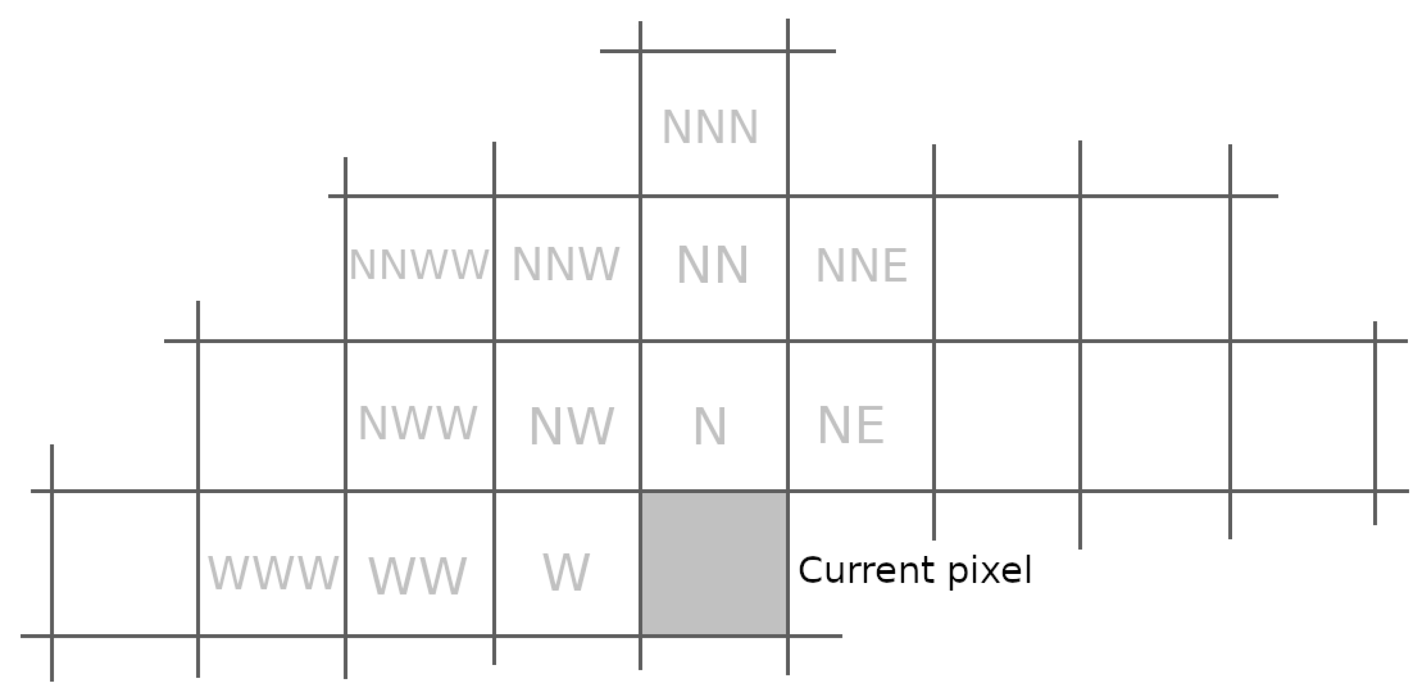
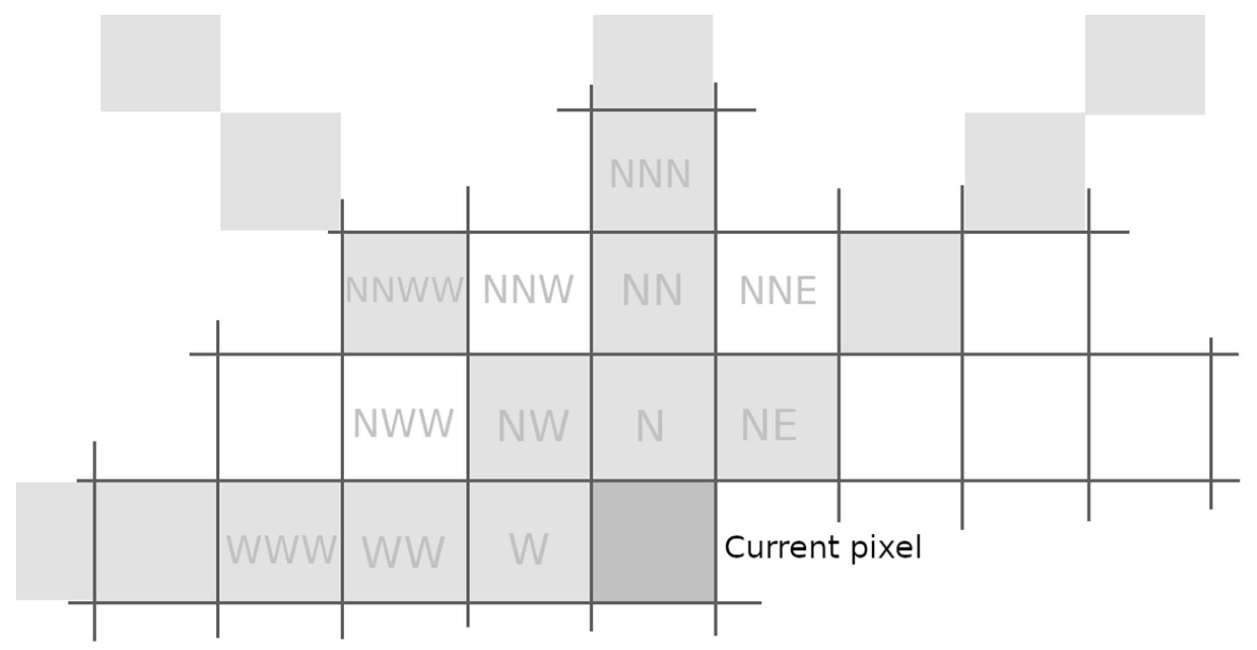
4.1. Context Modeling

When it comes to predictive compression, we need to decide what best describes the part of the image we are currently trying to predict. This means that we need to look around the target pixel in the hope that the information will be enough to help a decision mechanism recognize which part of the image we are in and choose to use the appropriate representation of the internally created segmentation of the image.

Before continuing, we need to define the terms used in Figure 3. The word context represents the region of the image that participates in the prediction mechanism. “Context value” is the numeric value of the context, either a direct value or a function of that value, which will be used as an index in the memory structure. The algorithm makes no assumption about the memory structure, but we provide some implementation details. The output of indexing the memory is the “memory value”.

We choose a simple model for contexts for predicting the bits of the pixels. We use rays in four directions and with various lengths, and the quantized derivatives along the rays. Since the pixels of the image are predicted from left to right, top to bottom, the only information we can rely on are known pixels, which means the directions are to the west, 45 degrees north-west, north, and 45 degrees north-east. The rays are depicted as gray background in Figure 4. We choose rays of varying lengths from length 1 to 7, but use this as a parameter. The derivative with respect to the intensity value is computed as the difference between the consecutive pixels of the ray and quantizing is done by masking the lower order bits from the derivative. We use three levels of quantizing, each cutting out one more bit than the other. The current pixel participates in the contexts only with the currently known bits.

In order to compute the context value from the contexts, we use a hashing function. We chose Fowler–Noll–Vo hash function (FNV) that is a non-cryptographic one byte at a time, designed to compute fast and with a low collisions rate. It is found to be particularly suited for hashing nearly identical strings [27].

As an optimization, since we know that we will need to compute hashes for rays, we exploit the fact that FNV computes one byte at a time hashes and pass as input only the longest ray and output all the intermediate results. We apply the same optimization for the quantized derivatives of the rays.

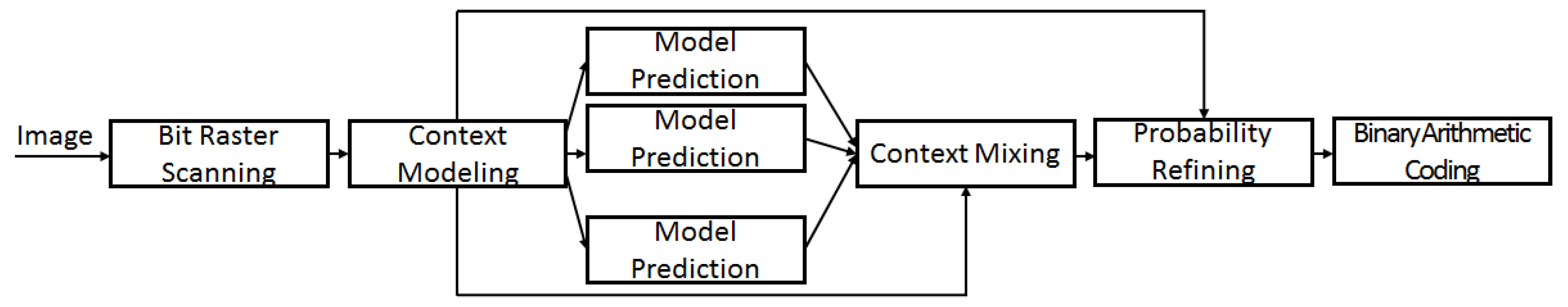
4.2. Description of the Contextual Prediction

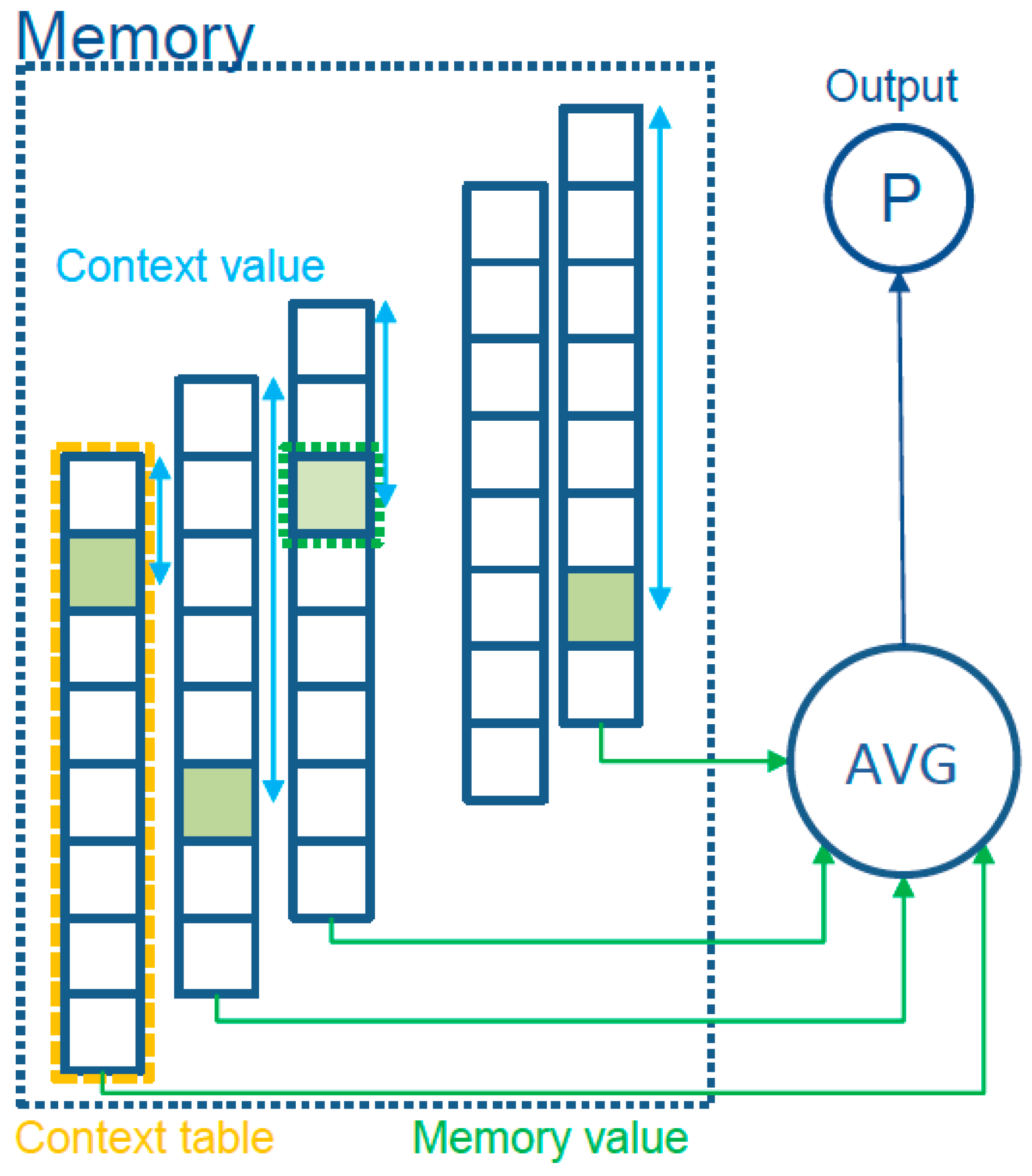
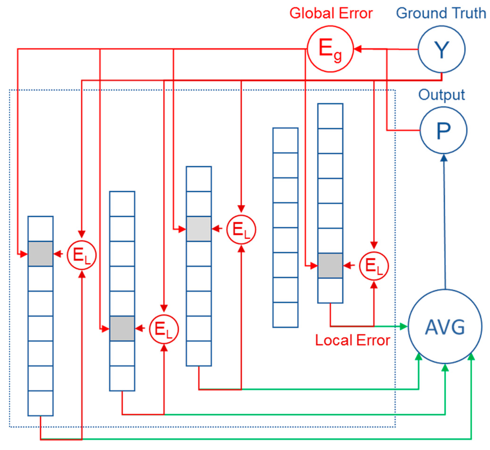
4.2.1. Model Prediction

To make a prediction, we propose the following algorithm (simplified from the original proposed algorithm [28], which had a probability refinement phase):

• We obtain a value from the memory for each context. One way to do that is to index the hash of the “context value” in a table
• We average all the obtained “memory values”
• Convert the average into a probability using the sigmoid function

  $$p=\sigma \left(\frac{k}{n}{\displaystyle \sum }_{i=0}^n{v}_i\right), v_i=M\left[i\right]\left[hash\left(c_i\right)\right]$$

  (3)

p is the output probability (that a bit is one),

n is the number of input contexts,

c_i is the context value of the i-th context,

v_i is the memory value from the memory M for context i,

k is some ad-hoc constant

σ is the sigmoid function.

4.2.2. Interpretation of Values

Logistic regression is a way of combining probabilities when they are fed as inputs to the algorithm. Using stretched probabilities as inputs (applying logit function to them), logistic mixing becomes optimal for minimizing wasted coding space (Kullback–Leibler divergence) [24] because the weighting becomes geometric.

$${\beta }_0+{\beta }_1{x}_{1,i}+{\beta }_2{x}_{2,i}+\cdots +{\beta }_0{x}_{k,i}$$

(4)

where $x_{j,i}$ is a probability, becomes

$${\beta }_0+{\beta }_1{t}_{1,i}+{\beta }_{2}t+\cdots +{\beta }_0{t}_{k,i}$$

(5)

where

$$t_{j,i}= \mathrm{logit}(x_{j,i})$$

(6)

The update formula for minimizing the relative entropy is:

$${\beta }_j={\beta }_j+ \alpha \ast t_j\ast \left(y_i-p_i\right)$$

(7)

The set of weights carries a part of the predictive part of the ensemble, and they get updated to better represent the potential of individual components. In the case of PAQ8, the components gather statistics independently and the network independently mixes the statistics. Adding more weights to the mixer can result in improved predictive power since the model can better discriminate between the contexts. But what if instead of separating the mixer from the statistics we move the mixing information towards the components? How can we pass the mixing information to the weak learners of the ensemble?

So far, we know that the memory value v_i is taken from a memory structure. The index in the memory is computed based on the context value. But the feature is the context, not the memory value. We can assume that the memory value is

$$v_i={\beta }_i\ast t_i$$

(8)

with t_i a stretched probability and β the weight of the probability in the ensemble. Computing the output probability resembles logistic regression, with the main difference being that we apply averaging. The average in itself is a weighted stretched probability

$$\frac{k}{n}{\displaystyle \sum }_{i=0}^n({\beta }_i\ast t_i)$$

(9)

which is converted into a regular probability by applying the sigmoid function.

4.2.3. Updating the Model

In order to pass mixing information to the weak learners, we propose a dual objective minimization function (as depicted in Figure 5):

• In respect to the output of the network–global error
• In respect to the output of the individual nodes (side predictions)–local error

Like PAQ8, we use reinforcement learning. Since we do not know the true value of the probability that a bit is 0 or 1 in a given context, we cannot use supervised learning. We backpropagate the binary outcome in the network and try to minimize the cumulative logistic loss in an online manner. The square loss can be also used, but we are trying to minimize the wasted coding space.

For minimizing the logistic loss, the formula we used for the global error is

$$E_g={\beta }_g\left(p-y\right)$$

(10)

If we wanted to minimize the square loss, the formula would be

$$E_g={\beta }_g\left(p-y\right)\ast p\ast \left(1-p\right)$$

(11)

with E_g as the global error, β_g the global error learning rate, p is the output probability of the entire network, and y the binary ground truth.

The local error is computed for each memory value in a similar fashion to the global error.

$$E_l= {\beta }_l\ast \left(p_i-y\right), p_{i=}\sigma \left(k_v\ast v_i\right)$$

(12)

with E_l as the local error, β_l the local error learning rate, p_i is the output probability for the i-th context (side prediction) multiplied by an ad-hoc value k_v, computed as the sigmoid of the memory value v_i, and y is the binary ground truth.

All the “memory values” are then updated by subtracting the local and global errors:

$$v_i=v_i-E_l-E_g$$

(13)

Instead of updating weights of the mixture, we update directly the values that contribute to the average. We have no layer to separate the context weights from the input probabilities, making the method different from the context mixing algorithm.

4.3. Memory Implementation and Variations

The algorithm makes no assumption on how to organize the memory structure. We describe here potential implementation and give more details to the implementation we chose to use. The proposed implementations are based on hash tables since they give fast retrieval, given the fact that the context values are computed by hashing series of pixel values. We chose the 32-bit FNV hashing with table sizes the power of two so that indexing an entry will be done by masking. We use separate tables for each context so we have collision independence. The difference between the memory types comes from the way collisions and new entries are treated.

• simple lookup–we ignore the potential collisions and average the memory values, multiply the result by an ad-hoc constant, and then apply the sigmoid function,

  $$p=\sigma \left(sum\ast c\right), c=\frac{k}{n}$$

  (14)

  where n is the number of contexts and k is an ad-hoc constant. Once the number of contexts becomes known, c becomes a constant and can be computed only once.
• tagged lookup–for each memory value a small tag is added that is computed by taking the higher order bits of the context value. If a table address size is less than 32 bits, the remaining bits still can bring value to the indexing. If the tag matches, we can use the value for the average.

  $$p=\sigma (\frac{sum\ast k}{n_t})$$

  (15)

  where n_t is the number of tag matches. In an empirical study we concluded that instead of simply averaging the values, we can get better results by dividing the sum by the average of the number of contexts and the number of tag matches. The formula becomes

  $$p=\rho \left(\frac{sum\ast k}{\frac{n_t+n}{2}}\right)$$

  (16)
  This is an approximate weighting of the confidence of the output based on how many inputs participate in the result.
  On update, we update the tag of the location where it does not match. The value of the location can be reset to zero or the old value can be kept and the regular updated formula used. Keeping the old value sometimes gives better results and we believe this is because the collisions generated by noise can reset a very biased context value. This method uses more memory and has a more complex update rule, but gives better results than the simple lookup with the cost of improved computing complexity.
• bucket lookup–the context value indexes a bucket with an array of tagged values. The selection of the memory value is done by searching the bucket for a matching tag. In this way, we can implement complex replacement rules for the values inside the bucket. We provide a “least bias” eviction rule when no tag is matched in the bucket. This means kicking the location with the value closest to zero. In this way, we keep the values that can bring benefits to the compression. Computing the output and the update rules are the same as in tagged lookup. If the bucket size is kept small (4 to 8 entries), the linear search is done in the same cache line, making the speed comparable to the tagged lookup.

The tests we performed yielded different results for the proposed memory implementations. Each implementation should be chosen by taking into account the balance of speed versus the quality of prediction (from the first to the third).

As an optimization, instead of having the memory values represented as floating point numbers that occupy 32 bits, we quantize the value to a fixed-point represented by a short integer that only uses 16 bits. In the future, we could replace this representation with the FP16 standard. For tagged values we have found that 8-bit values are enough, making the whole tag-value pair to be 24 bits. In this way, we can use lookup tables for computing the local error, since we know that the values are constricted to 65536 possibilities and we avoid the multiply and squash operations.

Memory implementations consider the 8 bits per byte structure of the image. This means that the buckets should be indexed using a proximity function for faster memory access. We used the XOR function of the initial context value hash with the partial known nibble (4 bits of a byte) to create a new index. This ensures that the new context value will fall inside the same (or at most another) cache line of 64 bytes. After 4 bits, a new hash is computed with the known full nibble.

5. Experimental Results

5.1. PAQ8PX Contextual Memory Implementation Details

We implemented the contextual memory algorithm for the 8 bpp lossless image compression. This section describes the architecture and some of the implementation details of the application.

The application is implemented in the C++ programming language, since the PAQ8PX was already implemented in this language. The code is compiled in Visual Studio and separates the original code, the changes required for compilation and the additional implementation into different commits, making clear which part is which.

The source code containing a full implementation of the algorithm will be publicly available at the GitHub page [29] repository [30].

5.2. Evaluation on the Benchmarks

In order to test the effectiveness of the algorithm, we applied the augmented version of the PAQ8PX algorithm with contextual memory to four test sets. The command line option for the compression for all the images selects memory level 8 and adaptive learning rate (-8a).

The Waterloo image compression benchmark [31] contains two test sets with image sizes from 256 x 256 pixels up to 1118 x 1105. For this benchmark, we used as parameters for the contextual memory ray length 5 and memory size 20. The results are presented in

Table 1. Waterloo gray test set 1.

Set	JPEG 2000	JPEG-LS	MRP	ZPAQ	VanilcWLS D	Paq8px167	Paq8px167+CM (proposed)
bird	3,6300	3,4710	3,2380	4,0620	2,7490	2,6073	2,6077
bridge	6,0120	5,7900	5,5840	6,3680	5,5960	5,5074	5,5037
camera	4,5700	4,3140	3,9980	4,7660	3,9950	3,8176	3,8173
circles11	0,9280	0,1530	0,1320	0,2300	0,0430	0,0281	0,0282
crosses1	1,0660	0,3860	0,0510	0,2120	0,0160	0,0176	0,0171
goldhill1	5,5160	5,2810	5,0980	5,8210	5,0900	5,0220	5,0197
horiz11	0,2310	0,0940	0,0160	0,1220	0,0150	0,0139	0,0140
lena1	4,7550	4,5810	4,1890	5,6440	4,1230	4,1302	4,1293
montage1	2,9830	2,7230	2,3530	3,3350	2,3630	2,1505	2,1501
slope1	1,3420	1,5710	0,8590	1,5040	0,9600	0,7186	0,7194
squares1	0,1630	0,0770	0,0130	0,1770	0,0070	0,0129	0,0128
text1	4,2150	1,6320	3,1750	0,4960	0,6210	0,1053	0,1052
Average	2,9510	2,5060	2,3920	2,7280	2,1310	2,0109	2,0103

_¹ Non-natural/artificially generated image

and

Table 2. Waterloo gray test set 2.

Set	JPEG2000	JPEG-LS	MRP	ZPAQ	VanilcWLS D	Paq8px167	Paq8px167+CM (proposed)
barb	4,6690	4,7330	3,9100	5,6720	3,8710	3,9319	3,9297
boat	4,4150	4,2500	3,8720	4,9650	3,9280	3,8165	3,8145
france1	2,0350	1,4130	0,6030	0,4220	1,1590	0,0992	0,0966
frog	6,2670	6,0490	_2	3,3560	5,1060	2,4656	2,4581
goldhill2	4,8470	4,7120	4,4650	5,2830	4,4630	4,4227	4,4214
lena2	4,3260	4,2440	3,9230	5,0660	3,8680	3,8608	3,8604
library1	5,7120	5,1010	4,7650	4,4870	4,9110	3,3253	3,3200
mandrill	6,1190	6,0370	5,6790	6,3690	5,6780	5,6364	5,6339
mountain	6,7120	6,4220	6,2210	4,4930	5,2150	4,0799	4,0744
peppers2	4,6290	4,4890	4,1960	5,0950	4,1740	4,1493	4,1470
washsat	4,4410	4,1290	4,1470	2,2900	1,8900	1,7478	1,7466
zelda	4,0010	4,0050	3,6320	4,9200	3,6330	3,6437	3,6435
Average	4,8480	4,6320		4,3680	3,9910	3,4316	3,4288

_¹ Non-natural/artificially generated image

_² Supported image size only multiple of eight

. A newer benchmark, Sachin Garg’s test images corpus [32], contains images ranging from 2268 x 1512 pixels up to 7216 x 5412. For this benchmark, we used ray length 7 and memory size 23 as parameters for the contextual memory. The results are presented in

Table 3. Imagecompression.info 8 bpp gray new test images.

Set	JPEG2000	JPEG-LS	MRP	ZPAQ	GraLIC	VanilcWLS D	Paq8px167	Paq8px167+CM (proposed)
artificial1	1,1970	0,7980	0,5170	0,6730	0,4464	0,6820	0,3188	0,3186
big_building	3,6550	3,5920	_2	4,3350	3,1777	3,2430	3,1250	3,1216
big_tree	3,8050	3,7320	_2	4,4130	3,4080	3,4680	3,3823	3,3803
Bridge	4,1930	4,1480	_2	4,7250	3,8700	3,8420	3,7958	3,7953
cathedral	3,7100	3,5700	3,2600	4,2390	3,1900	3,3020	3,1539	3,1519
Deer	4,5820	4,6590	_2	4,7280	4,3116	4,3760	4,1788	4,1750
fireworks	1,6540	1,4650	1,3010	1,5550	1,2500	1,3640	1,2324	1,2325
flower_foveon	2,1980	2,0380	_2	2,4640	1,7761	1,7470	1,6944	1,6943
hdr	2,3440	2,1750	1,8540	2,5890	1,9197	1,8730	1,8330	1,8327
leaves_iso_200	4,0830	3,8200	3,4000	4,7430	3,2630	3,5370	4,0509	4,0473
leaves_iso_1600	4,6810	4,4860	4,1860	5,2600	4,0720	4,2430	3,2168	3,2130
nightshot_iso_100	2,3000	2,1300	1,8390	2,5760	1,8240	1,8750	1,7811	1,7805
nightshot_iso_1600	4,0380	3,9710	3,7430	4,2680	3,6610	3,7820	3,6295	3,6272
spider_web	1,9080	1,7660	1,3490	2,3640	1,4441	1,4220	1,3498	1,3502
zone_plate1	5,7550	7,4290	2,8340	5,9430	0,8620	0,9110	0,1257	0,1257
Average	3,3400	3,3190		3,6580	2,5650	2,6500	2,4579	2,4564

_¹ Non-natural/artificially generated image

_² Supported image size only multiple of eight

. We also included the Squeezechart 8 bpp grayscale images test set [33] where four of the five images are medical images. For this benchmark, we used ray length 6 and memory size 20 as parameters for the contextual memory. The results are presented in

Table 4. Squeezechart 8 bpp grayscale.

Set	MRP	cmix v14f	GraLIC	Paq8px167	Paq8px167+CM (proposed)
blood8	2,1670	2,1600	2,3200	2,1308	2,1304
cathether8	1,5350	1,5351	1,6580	1,5382	1,5380
fetus	4,0650	3,9730	4,1310	3,8236	3,8225
shoulder	2,8660	2,9080	3,1130	2,8697	2,8676
sigma8	2,6870	2,6290	2,7200	2,6266	2,6263
Average	2,6640	2,6410	2,7880	2,5978	2,5970

. The best results in the table are highlighted using bold font weight.

We used as learning constants global learning rate βg = 0.9 and local learning rate β_l = 0.1 and the constants k and k_v were set to 0.4.

The results in Table 1, Table 2, Table 3 and Table 4 are expressed in bits per pixel which is an image size independent absolute measure of the compression ratio. It represents the average number of bits needed to encode the pixel information from an image. It is computed as the compressed size of the image divided by the number of pixels. This is not to be confused with bits per byte, which measures the compressed ratio of a general file, though in our case the two values coincide since the size of a pixel in an 8-bit color depth grayscale image is one byte. The header of the compressed file should be excluded when computing the bits per pixel, but it is not always the case since the header is usually a minor payload compared to the content. However, it should be specified if the header is included or not in computing the bits per pixel so that the results can be verified.

5.3. Discussion on the Results

The reason for choosing these benchmarks is that they are publicly available and that they are provided without conflicts of interest. They contain images of various types such as artificially generated, edited, photographs, and scans. This makes them suitable for publications and there are published papers using them, such as [11]. We present our results on all the images in the datasets in order to prove that we did not tune the algorithm to a selected few. The images are compressed separately (as in not a solid archive) to prevent reusing correlations.

The PAQ8 family of algorithms was designed to achieve good compression ratios at the expense of a long compression time and a large memory footprint. Even though there are some optimizations applied, the running time will be much larger than some of the other algorithms. The contextual memory algorithm also does not contain too many speed optimizations in its provided form. Therefore, a running time comparison is out of the scope of this paper, but to give the reader a sense of the execution time scale, we provide a relative comparison on the image lena2 from the Waterloo gray test set (see

Table 5. Compression running time comparison on image lena2 (expressed in seconds).

Image	MRP	JPEG 2000	JPEG-LS	GraLIC	Paq8px167	Paq8px167+CM (proposed)
lena2	258 s	0.04 s	0.02 s	0.25 s	12 s	24 s

). The algorithms where run on the same processing architecture.

The compression running time does not equal the decompression running time for all the algorithms. For instance, the MRP algorithm is highly asymmetric due to its multiple pass optimizations, decompression of the same image taking only 0.6 seconds. The timings were measured using the x64 version of the Timer 14.00 tool created by Igor Pavlov and available for public domain on the 7-cpu website [34].

Memory requirements depend on the compression parameters. PAQ8PX reports using 2493MB of memory for command line parameter -8a. The contextual memory algorithm adds to this depending on the parameters set. We can estimate the memory consumption of the current implementation by multiplying the number of rays by ray length, table size (2^{memory size}), 4 (no quantization plus 3 quantized derivatives), 3 (number of bytes per memory location). For ray length 5 and memory size 20, we estimate that it adds another 240 MB of memory.

The results in Table 1, Table 2 and Table 3 for all the compressors, except Paq8px167 and the proposed method, were taken directly from [11], and the results in Table 4 were taken from the PAQ8PX thread [21]. The results missing in the paper for GraLIC and the results for Paq8px167 and the proposed method are computed using a tool we created for this purpose, available at [35]. The tool does not exclude the file headers when computing the bits per pixel.

6. Conclusions and Future Work

This paper provides a description of the state-of-the-art compression program PAQ8PX from the point of view of grayscale image compression. The main contribution of this paper is an application agnostic algorithm for predicting probabilities based on the contextual information available with learning done in an online fashion. The usefulness of the algorithm is demonstrated by integrating it with the PAQ8PX algorithm and testing it on several image compression benchmarks. The results show an overall compression ratio improvement across all the datasets without special crafted features. One important difference from existing ensemble mixing algorithms is that, in our algorithm, we assume that various contexts apply together and the prediction benefits from the synergy of the side predictions, unlike the ensembles that assume model independence.

In its current state, the algorithm was not applied to color or 16 bpp images. For future developments, we intend to extend the algorithm for three-dimensional medical image compression and support 16 bpp depth. Context modeling can be done similarly to the work described in [15].

The architecture chosen for the algorithm does not take into account parallel optimization techniques that are suitable for hardware implementation like the CCSDS developed image compression algorithms [17]. Unlike the CCSDS standard, the focus for PAQ8 is set to provide the unconstrained liberty for exploring techniques to improve the compression ratio. However, if one wants to standardize an epoch of development, the code can be converted to the ZPAQ open standard [36] that, among other things, aims for forward and backward compatibility of archives. Although not presented in this paper, in future releases we can compare the compression ratio with the CCSDS family of algorithms.

In [37], a context function is proposed to statistically discriminate error residual classes of full pixel prediction, useful for lossless and near-lossless compression schemes. Due to its properties, such a function could be integrated within the context mixing layer and the adaptive probability maps.

Design space exploration needs to be done for context modeling. Moving contexts from other modeling types to the contextual memory predictor might also bring benefits. The side predictions of the algorithm can be also be passed to the context mixing network. Splitting various contexts into two or more contextual memory structures can also lead to finding better correlations.

References

- Chen, D.; Li, Y.; Zhang, H.; Gao, W. Invertible update-then-predict integer lifting wavelet for lossless image compression. EURASIP J. Adv. Signal Process. 2017, 2017, 8–17. [Google Scholar] [CrossRef]
- Khan, A.; Khan, A.; Khan, M.; Uzair, M. Lossless image compression: Application of Bi-level Burrows Wheeler Compression Algorithm (BBWCA) to 2-D data. Multimed. Tools Appl. 2017, 76, 12391–12416. [Google Scholar] [CrossRef]
- Feng, W.; Hu, C.; Wang, Y.; Zhang, J.; Yan, H. A Novel Hierarchical Coding Progressive Transmission Method for WMSN Wildlife Images. Sensors 2019, 19, 946. [Google Scholar] [CrossRef] [PubMed]
- Schiopu, I.; Munteanu, A. Residual-error prediction based on deep learning for lossless image compression. Electron. Lett. 2018, 54, 1032–1034. [Google Scholar] [CrossRef]
- Hosseini, S.M.; Naghsh-Nilchi, A.-R. Medical ultrasound image compression using contextual vector quantization. Comput. Biol. Med. 2012, 42, 743–750. [Google Scholar] [CrossRef] [PubMed]
- Eben Sophia, P.; Anitha, J. Contextual Medical Image Compression using Normalized Wavelet-Transform Coefficients and Prediction. IETE J. Res. 2017, 63, 671–683. [Google Scholar] [CrossRef]
- Borusyak, A.V.; Vasin, Y.G. Development of an algorithm for adaptive compression of indexed images using contextual simulation. Pattern Recognit. Image Anal. 2016, 26, 4–8. [Google Scholar] [CrossRef]
- Strutz, T. Context-Based Predictor Blending for Lossless Color Image Compression. IEEE Trans. Circuits Syst. Video Technol. 2016, 26, 687–695. [Google Scholar] [CrossRef]
- Knezovic, J.; Kovac, M.; Mlinaric, H. Classification and Blending Prediction for Lossless Image Compression. In Proceedings of the MELECON 2006–2006 IEEE Mediterranean Electrotechnical Conference, Benalmadena, Spain, 16–19 May 2006; pp. 486–489. [Google Scholar] [CrossRef]
- Strizic, L.; Knezovic, J. Optimization of losless image compression method for GPGPU. In Proceedings of the 18th Mediterranean Electrotechnical Conference (MELECON), Lemesos, Cyprus, 18–20 April 2016; pp. 1–6. [Google Scholar] [CrossRef]
- Weinlich, A.; Amon, P.; Hutter, A.; Kaup, A. Probability Distribution Estimation for Autoregressive Pixel-Predictive Image Coding. IEEE Trans. Image Process. 2016, 25, 1382–1395. [Google Scholar] [CrossRef] [PubMed]
- Biadgie, Y.; Kim, M.; Sohn, K.-A. Multi-resolution Lossless Image Compression for Progressive Transmission and Multiple Decoding Using an Enhanced Edge Adaptive Hierarchical Interpolation. Ksii Trans. Internet Inf. Syst. 2017, 11, 6017–6037. [Google Scholar] [CrossRef]
- Biadgie, Y. Edge Adaptive Hierarchical Interpolation for Lossless and Progressive Image Transmission. Ksii Trans. Internet Inf. Syst. 2011, 5, 2068–2086. [Google Scholar] [CrossRef]
- Song, X.; Huang, Q.; Chang, S.; He, J.; Wang, H. Lossless medical image compression using geometry-adaptive partitioning and least square-based prediction. Med Biol. Eng. Comput. 2018, 56, 957–966. [Google Scholar] [CrossRef] [PubMed]
- Lucas, L.F.R.; Rodrigues, N.M.M.; da Silva Cruz, L.A.; de Faria, S.M.M. Lossless Compression of Medical Images Using 3-D Predictors. IEEE Trans. Med. Imaging 2017, 36, 2250–2260. [Google Scholar] [CrossRef] [PubMed]
- Shen, H.; Jiang, Z.; Pan, W. Efficient Lossless Compression of Multitemporal Hyperspectral Image Data. J. Imaging 2018, 4, 142. [Google Scholar] [CrossRef]
- Consultative Committee for Space Data Systems CCSDS Recommended Standard for Image Data Compression. 2017. Available online: https://public.ccsds.org/Pubs/122x0b2.pdf (accessed on 29 June 2019).
- Knoll, B.; De Freitas, N. A Machine Learning Perspective on Predictive Coding with PAQ8. In Proceedings of the 2012 Data Compression Conference, Snowbird, UT, USA, 10–12 April 2012; pp. 377–386. [Google Scholar] [CrossRef]
- Mahoney, M.V. Adaptive Weighing of Context Models for Lossless Data Compression; The Florida Institute of Technology: Melbourne, FL, USA, 2005; Volume 6. [Google Scholar]
- Data Compression Explained. Available online: http://mattmahoney.net/dc/dce.html#Section_43 (accessed on 11 May 2019).
- Paq8px thread. Available online: https://encode.ru/threads/342-paq8px (accessed on 11 May 2019).
- Chartier, M. MCM File Compressor. Available online: https://github.com/mathieuchartier/mcm (accessed on 29 June 2019).
- Veness, J.; Lattimore, T.; Bhoopchand, A.; Grabska-Barwinska, A.; Mattern, C.; Toth, P. Online Learning with Gated Linear Networks. arXiv 2017, arXiv:1712.01897 [cs, math]. [Google Scholar]
- Mattern, C. Mixing Strategies in Data Compression. In Proceedings of the 2012 Data Compression Conference, Snowbird, UT, USA, 10–12 April 2012; pp. 337–346. [Google Scholar] [CrossRef]
- Mattern, C. Linear and Geometric Mixtures-Analysis. In Proceedings of the 2013 Data Compression Conference, Snowbird, UT, USA, 20–22 March 2013; pp. 301–310. [Google Scholar] [CrossRef]
- Mattern, C. On Statistical Data Compression. Ph.D. Thesis, Technische Universität Ilmenau, Ilmenau, Germany, 2016. [Google Scholar]
- Fowler–Noll–Vo Hash Functions. Available online: http://www.isthe.com/chongo/tech/comp/fnv/index.html (accessed on 11 May 2019).
- Dorobanţiu, A.; Brad, R. A novel contextual memory algorithm for edge detection. Pattern Anal. Appl. 2019, 1–13. [Google Scholar] [CrossRef]
- Alexandru Dorobanțiu-GitHub. Available online: https://github.com/AlexDorobantiu (accessed on 11 May 2019).
- Dorobanțiu, A. Paq8px167ContextualMemory. Available online: https://github.com/AlexDorobantiu/Paq8px167ContextualMemory (accessed on 13 May 2019).
- Image Repository of the University of Waterloo. Available online: http://links.uwaterloo.ca/Repository.html (accessed on 11 May 2019).
- Garg, S. The New Test Images-Image Compression Benchmark. Available online: http://imagecompression.info/test_images/ (accessed on 11 May 2019).
- Squeeze Chart Lossless Data Compression Benchmarks. Available online: http://www.squeezechart.com/ (accessed on 11 May 2019).
- 7-cpu. Available online: https://www.7-cpu.com/utils.html (accessed on 13 June 2019).
- Dorobanțiu, A. Compute Bits Per Pixel for Compressed Images. Available online: https://github.com/AlexDorobantiu/BppEvaluator (accessed on 29 June 2019).
- Mahoney, M. The ZPAQ Open Standard Format for Highly Compressed Data-Level 2. 2016. Available online: http://www.mattmahoney.net/dc/zpaq206.pdf (accessed on 29 June 2019).
- Aiazzi, B.; Alparone, L.; Baronti, S. Context modeling for near-lossless image coding. IEEE Signal Process. Lett. 2002, 9, 77–80. [Google Scholar] [CrossRef]