Featured Application
This work is used for the unmanned driving of vehicles and other devices.
Abstract
At present, many path tracking controllers are unable to actively adjust the longitudinal velocity according to path information, such as the radius of the curve, to further improve tracking accuracy. For this problem, we propose a new path tracking framework based on model predictive control (MPC). This is a multilayer control system that includes three path tracking controllers with fixed velocities and a velocity decision controller. This new control method is named multilayer MPC. This new control method is compared to other control methods through simulation. In this paper, the maximum values of the displacement error and the heading error of multilayer MPC are 92.92% and 77.02%, respectively, smaller than those of nonlinear MPC. The real-time performance of multilayer MPC is very good, and parallel computation can further improve the real-time performance of this control method. In simulation results, the calculation time of multilayer MPC in each control period does not exceed 0.0130 s, which is much smaller than the control period. In addition, when the error of positioning systems is at the centimeter level, the performance of multilayer MPC is still good.
1. Introduction
An autonomous vehicle system usually consists of mapping, positioning, perception, and navigation. Path tracking is a core system of the autonomous navigation system. Its task is to control the vehicles devices to track the reference path by minimizing errors [1,2,3,4]. Based on our previous work [5], this paper still focuses on the path tracking of articulated vehicles. Of course, the control method proposed in this paper can also be applied in the path tracking of mobile devices such as front-wheel steering vehicles and differential robots.
1.1. Motivations
The motivation for this paper is to further improve the accuracy of path tracking. In previous work, we found that most path tracking methods cannot adjust the velocity of the vehicle according to path information such as the radius of the curve, and a high reference velocity at corners will lead to a sharp deterioration in path tracking performance [5].
There is no doubt that path tracking controllers perform well at a low reference velocity. However, too low driving efficiency is also unacceptable in the mining industry. So, when should the articulated vehicle slow down? How much should it reduce its velocity by? It is difficult to calculate the most suitable reference velocity for each curve. For the above problems, we propose multilayer model predictive control (multilayer MPC) for the path tracking of articulated vehicles. This controller can adjust the velocity according to the path information.
1.2. Related Works
Currently, there are many control methods for the path tracking of articulated vehicles. Feedback linearization control and optimal control are the most common of these.
The history of path tracking for articulated vehicles based on feedback linearization control is very long. Hemami et al. designed controllers in this way earlier [6,7,8]. DeSantis et al. proposed a similar controller in 1997 [9]. Based on the classic kinematics model of articulated vehicles, Corke et al. also designed a controller using feedback linearization control [10]. Until 2019, there are still new controllers based on feedback linearization [11,12,13,14,15].
Feedback linearization control is a mature traditional control method, however its shortcomings are also obvious. The parameters of feedback linearization controllers are usually fixed, however the reference path is complex and diverse, so consequently feedback linearization controllers often perform poorly when tracking complex reference paths. Nayl et al. have proven that the performance of feedback linearization control is not as good as that of model predictive control (MPC) [16,17,18].
MPC is a kind of optimal control method. Linear quadratic regulation (LQR) is the other optimal control method that is often used for path tracking in articulated vehicles [19,20,21,22,23]. However, Nayl et al. have also demonstrated that MPC performs better than LQR. In addition, other researchers have also found that MPC performs better than LQR in the path tracking of front-wheel steering vehicles [24,25]. The reason why MPC performs better is that this control method can handle system constraints well and can add the feedforward information of the reference path.
However, in previous studies, we found that MPC is not perfect. Like feedback linearization and LQR, Nayl et al.’s switching MPC and our nonlinear MPC also cannot adjust the velocity in a wide range [5]. However, the accuracy of the path tracking control can be greatly improved by reducing the velocity during steering. Therefore, we believe that it is necessary to propose a new controller for the path tracking of articulated vehicles.
1.3. Contributions
In this paper, our contributions are listed as follows: Firstly, the multilayer MPC controller that can automatically adjust the velocity according to path information is proposed. Our proposed controller is compared with the switching MPC controller and the nonlinear MPC controller. The performance of the multilayer MPC controller is very good. Secondly, two controller topology schemes are proposed, and we prove that the parallel layout can further improve the real-time performance of multilayer MPC. Thirdly, the performance of the multilayer MPC controller under the impact of positioning error is verified.
2. Controller Design
The design of the controller consisted of three steps. First, we propose a framework for multilayer MPC, then, we design the first layer controllers and finally the second layer controller.
2.1. The Framework for Multilayer MPC
In our previous work [5] we found that most path tracking controllers can only adapt to different reference velocities and cannot regulate the operation velocity automatically. The reason for this phenomenon is that in many path tracking controllers, the state of the path tracking systems is partly determined by the reference velocity.
The performance of the controller varies greatly at different reference velocities. We guess that it is possible to get control inputs at different reference velocities through several controllers. These controllers are the first layer of the multilayer MPC, and we name them as path tracking controllers with a fixed velocity. As shown in Figure 1, we set up three path tracking controllers with fixed velocities in the multilayer MPC framework.
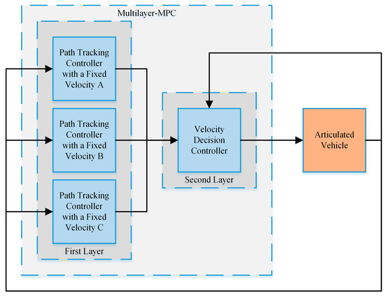
Figure 1.
The framework of multilayer model predictive control (MPC).
In these three controllers:
where is the reference velocity in the current control period, is the reference velocity in the last control period, and is the acceleration amplitude or deceleration amplitude based on constraints and control period. In addition:
where is the acceleration limit and is the control period.
These three controllers can generate three sets of control inputs. Due to constraints such as the upper limit of the articulated angle speed, sometimes these inputs cannot completely eliminate errors between the articulated vehicle and the reference path. By comparing these residual errors it is possible to decide which set of control inputs can make the path tracking control system perform better. Therefore, the second layer controller is a velocity decision controller.
2.2. Path Tracking Controller with a Fixed Velocity
Linear model predictive control (linear MPC) is very powerful in terms of its real-time performance, and it also has high accuracy when the reference velocity is low [26]. Consequently, we chose the linear MPC controller as the path tracking controller with a fixed velocity. In the process of designing this controller, we also referred to the work of Gong et al. [27] and Plessen et al. [28]. The linear MPC controller includes two parts, the predictive model and the rolling optimization. Except for the reference velocities, the three linear MPC controllers are identical.
The basis of the predictive model is the kinematic model of articulated vehicles. We still use the model in [5]. This model is very mature and its application is very extensive. In this kinematics model, we ignore the force of the tires and consider the bodies of the articulated vehicle as rigid bodies. The kinematics model is presented in Figure 2. The definition of the parameters is presented in [5].
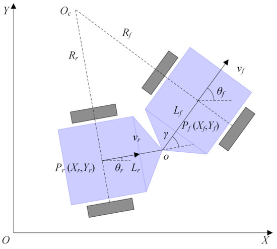
Figure 2.
Model of the articulated vehicle.
The matrix form of the kinematic model is:
where is the articulated angular speed.
Carrying out Jacobian linearization on Equation (3), the result is:
where:
In the path tracking controller with a fixed velocity, the reference velocity is the longitudinal velocity, so:
In Equations (5) and (6), is the -th predicted state at the current time , and is the -th possible control input at the current time . Especially, when , and are the state and control input of the last control period, respectively.
If the prediction horizon is , the control horizon is :
To make the relationship clearer, the future output of the system can be represented in a matrix:
where:
Since the function of the controllers is to enable articulated vehicle to track the reference path as quickly and smoothly as possible, the objective function of the rolling optimization can be designed as:
where is the linearized state information of the tracking target point, and are the weight matrices, is the relaxation factor, and is the weight factor.
We can rewrite Equation (15) as:
The tracking target point is the closest point to the articulated vehicle which is selected on the reference path. We can set its status information to , , , and . Then, we can set that:
So:
Then Equation (16) can be rewritten as:
If:
We can rewrite Equation (19) as:
where:
Combined with the constraints in [5], the final rolling optimization function is:
We can use the quadprog function in MATLAB to solve Equation (23), and the solution algorithm can be specified as active-set. After the solution, the control input increment sequence in the control time domain can be obtained:
2.3. Velocity Decision Controller
The function of the velocity decision controller is to judge the three sets of control inputs. This controller is not required to stand out in terms of real-time performance, as there is no large-scale optimization solution. Instead, this controller is required to accurately predict the state of the articulated vehicle in a long time domain. According to these requirements, we believe that nonlinear MPC is well suited for velocity decision controllers.
The kinematics model detailed in Equation (3) can be abbreviated as:
where:
After discretization, a nonlinear prediction model can be obtained:
Substituting the three sets of control inputs obtained in the first layer into Equation (27), the corresponding future state of the articulated vehicle can be obtained.
The errors between the reference path and the future state of articulated vehicles are:
where is the prediction horizon in the velocity decision controller and is the information on the reference path. is obtained by the interpolation of the reference path, based on the reference velocity and control period. The arc length on the reference path between and is equal to the product of the reference velocity and the control period.
Based on the above prediction model, the following decision function can be designed:
In order to ensure safety, the path tracking controller with the slowest velocity is set at the highest priority. The judgment rules are as follows:
where and are relaxation factors.
3. Simulation
The simulation environment used in this paper is exactly the same as in our previous work [5]. The parameters of the model and the controller are shown in Table 1. Figure 3 shows the definition of displacement error and heading error. Their detailed explanation can be found in [5].

Table 1.
Parameter values.
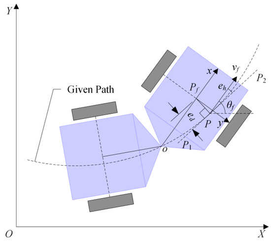
Figure 3.
Displacement error and heading error.
The simulation was divided into three groups. The first group is the comparison between the multilayer MPC controller, the nonlinear MPC controller and the switching MPC controller. The second group is the comparison between the two topologies of the multilayer MPC controller, and the third group is a performance test of the controller with positioning errors. In all simulations, most of the parameters were fixed. Each group simulation had the same computer model of articulated vehicles and the same reference path. The reference path consisted of straight lines and arcs, where the radius of the arcs was 10 m. The radius of these arcs is 5 m smaller than the radius of the arcs in [5].
3.1. Comparison Between Controllers
Firstly, multilayer MPC, switching MPC, and nonlinear MPC are compared. The reference velocity of the multilayer MPC controller was set to 5 m/s, and that of the other two controllers was set to 2.5 m/s. Figure 4 shows the tracking results. Multilayer MPC and switching MPC successfully completed the control task, however, switching MPC failed. According to [5,16,17,18], switching MPC can complete path tracking when the reference velocity is low or the radius of the reference path is large.
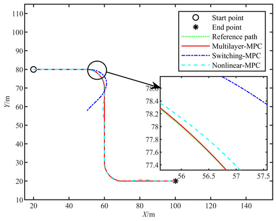
Figure 4.
The trajectory of the comparison between controllers.
Figure 5, Figure 6 and Figure 7 show the longitudinal velocity, articulated angle, and articulated angle speed, respectively. All control inputs and states are within the system constraints. The displacement error is shown in Figure 8. The heading error is shown in Figure 9. The errors of switching MPC are divergent. The maximum errors of the other controllers are shown in Table 2. The maximum displacement and heading errors of multilayer MPC are 92.92% and 77.02% smaller than those of nonlinear MPC, respectively.
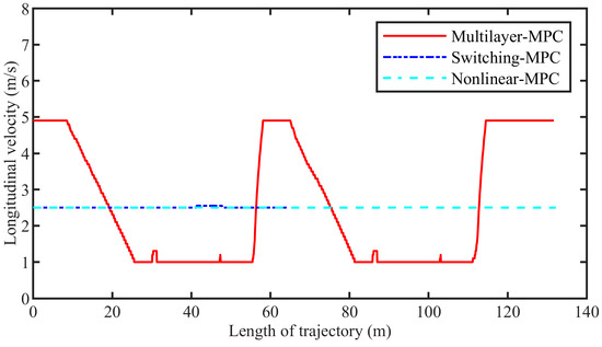
Figure 5.
The longitudinal velocity of the comparison between controllers.
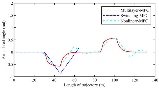
Figure 6.
The articulated angle of the comparison between controllers.
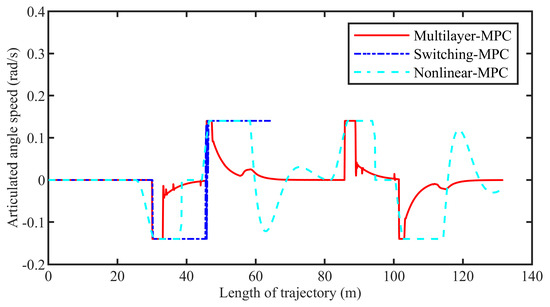
Figure 7.
Articulated angle speed of the comparison between controllers.
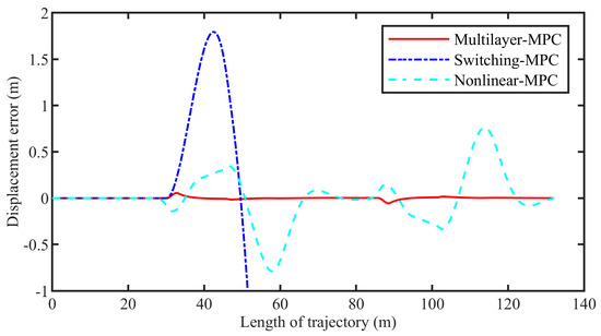
Figure 8.
Displacement error of the comparison between controllers.
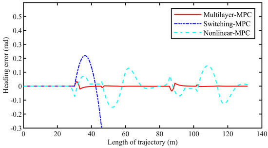
Figure 9.
Heading error of the comparison between controllers.
Table 2.
Maximum errors.
Multilayer MPC shows strong real-time performance, as shown in Figure 10. Its maximum calculation time in each control period was 0.0130 s, and its average calculation time was 0.0086 s. The real-time performance of multilayer MPC is significantly better than that of nonlinear MPC. Of course, the best control method for real-time performance is switching MPC, but this control method cannot control the articulated vehicle tracking reference path under this simulation condition.
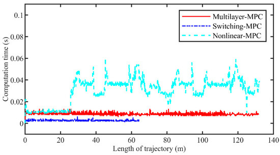
Figure 10.
The computation time of the comparison between controllers.
By comparing these control methods, we can see that multilayer MPC has good control precision and real-time performance. From a theoretical point of view, this controller can automatically adjust velocity according to the reference path.
3.2. Sequential Computation and Parallel Computation
Multilayer MPC is a distributed control method, so there are multiple topologies. The simplest two are sequential and parallel. These two calculation processes are shown in Figure 11. Of course, multi-threaded computing hardware is the basis of parallel computation.
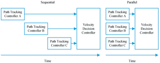
Figure 11.
Two calculation processes of multilayer MPC.
From a theoretical point of view, sequential computation and parallel computation only have an effect on real-time performance but have no effect on control accuracy. In a trajectory figure similar to Figure 4, it is difficult to observe the difference between the two topologies. So, in this group of simulations, we will compare the control inputs and states.
Figure 12, Figure 13, Figure 14, Figure 15 and Figure 16 show the longitudinal velocity, articulated angle, articulated angle speed, displacement error, and heading error, respectively. In theory, the variables of the two topologies should be identical. In the simulation, there were some deviations on a small scale. This phenomenon is caused by factors such as the sampling interval in the simulation.
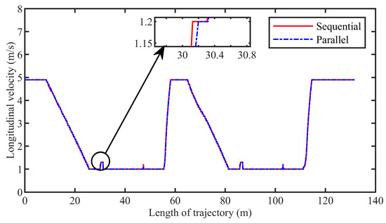
Figure 12.
The longitudinal velocity of the comparison between calculation processes.
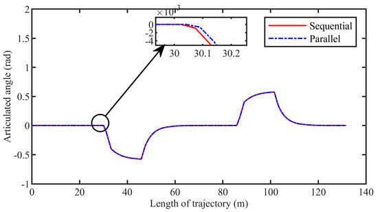
Figure 13.
The articulated angle of the comparison between calculation processes.
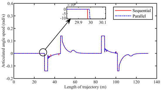
Figure 14.
Articulated angle speed of the comparison between calculation processes.
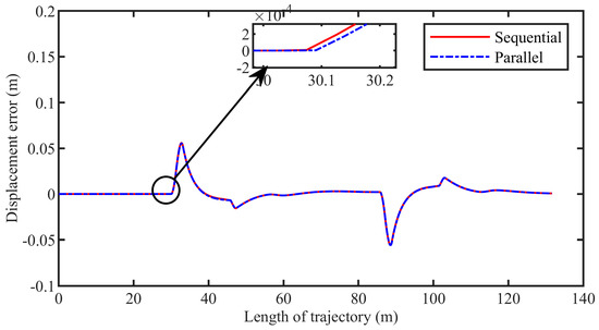
Figure 15.
Displacement error of the comparison between calculation processes.
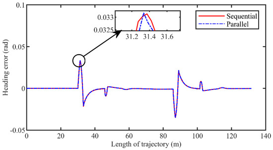
Figure 16.
Heading error of the comparison between calculation processes.
The real-time performance of parallel computation is obviously better than that of sequential computation, as shown in Figure 17. The maximum computation time for parallel computation was 0.0090 s, which was 30.77% smaller than that of sequential computation. The average computation time for parallel computation was 0.0044 s, which was 48.84% less than that of the sequential computation.
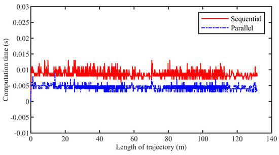
Figure 17.
The computation time of the comparison between calculation processes.
3.3. Performance with Positioning Error
The purpose of this group is to verify the performance of the controller with positioning errors.
At present, positioning devices such as BDM670 of Beijing BDStar Navigation Co. Ltd can provide centimeter-level positioning. Consequently, we added a random error within ± 0.01 m to the horizontal and vertical coordinates of the articulated vehicle model. Since the judgment of Equation (30) is based on errors, positioning errors will affect the function. To avoid the articulated vehicle always traveling at the minimum of the reference velocity, we increased and . In this group, was 4 and was 2.
Figure 18, Figure 19, Figure 20, Figure 21, Figure 22, Figure 23 and Figure 24 show the results of this group of simulations. The trend of each variable with positioning error was the same as the trend of the ideal variable. Therefore, we believe that multilayer MPC can be used in a working environment with small positioning errors.
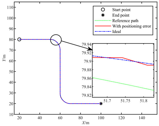
Figure 18.
The trajectory of the simulation with positioning errors.
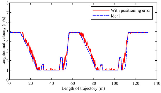
Figure 19.
The longitudinal velocity of the simulation with positioning errors.
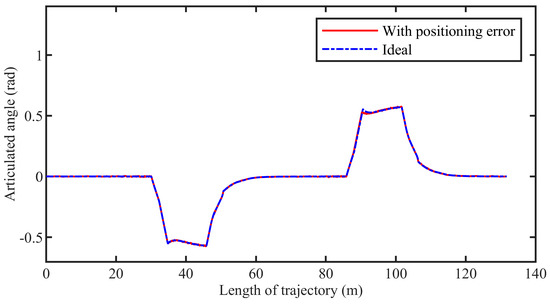
Figure 20.
The articulated angle of the simulation with positioning errors.
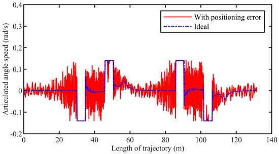
Figure 21.
Articulated angle speed of the simulation with positioning errors.
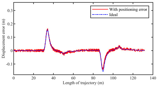
Figure 22.
Displacement error of the simulation with positioning errors.
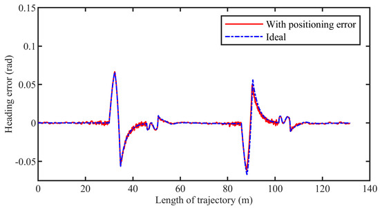
Figure 23.
Heading error of the simulation with positioning errors.
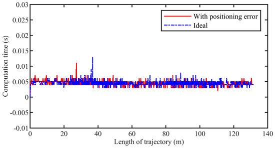
Figure 24.
The computation time of the simulation with positioning errors.
In addition, multilayer MPC still faces some challenges. As Figure 21, The articulation angle speed is not smooth due to the influence of the positioning error. Of course, this is a phenomenon that cannot be avoided by any controller, but we think there is still the possibility of improvement here. We believe that nonlinear MPC is more robust than linear MPC. If the linear MPC-based path tracking controller in multilayer MPC is replaced with the nonlinear MPC controller, the amplitude of the articulated angle speed may be reduced. However, the real-time performance of nonlinear MPC is suboptimal, requiring further work in the future solve this problem.
4. Conclusions
In our previous work [5] we found that switching model predictive control (MPC), nonlinear MPC, and most other control methods can operate at different longitudinal velocities but cannot actively adjust the longitudinal velocity according to the given path information. However, when tracking the same reference path, the tracking accuracy can be significantly improved by reducing the longitudinal velocity. To solve this problem, we propose a new MPC control method and name it multilayer MPC.
From the perspective of science, our contribution is to propose an MPC control framework that can actively adjust the longitudinal velocity according to the path information when path tracking. This is an exploration and development of MPC. We think that this framework can be applied to the control of other automated equipment.
From an engineering perspective we present many contributions. Firstly, we have demonstrated that the accuracy of path tracking can be improved by adjusting the longitudinal velocity. Compared with the nonlinear MPC controller, the multilayer MPC controller, which can actively adjust the longitudinal velocity, reduces the maximum displacement error by 92.92% and reduces the maximum heading error by 77.02%. Secondly, the real-time performance of multilayer MPC is very good. Moreover, compared with sequential computation, multilayer MPC with parallel computation has better real-time performance and its maximum calculation time is 0.0090 s. Thirdly, the multilayer MPC controller can still perform the path tracking task under the impact of positioning error.
Of course, there are still some shortcomings in our work. Firstly, limited by the lack of equipment, multilayer MPC has not been verified by real vehicles. We are deeply sorry about this issue, but the problem of acquiring or developing experimental equipment is difficult to solve quickly. We will work hard and try our best to provide the experiment as soon as possible. In addition, for positioning errors, the robustness of linear MPC in multilayer MPC does not satisfy us. We will solve this problem in our future work.
Author Contributions
Conceptualization, G.B., Q.G., and Y.M.; Methodology, G.B. and Q.G.; Software, G.B.; Validation, G.B., and K.L.; Investigation, G.B.; Writing-original draft preparation, G.B.; Writing-review and editing, Y.M., L.L., W.L., and Q.G.; Supervision, L.L. and W.L.; Project administration, L.L. and W.L.; Funding acquisition, L.L., W.L., Y.M., and Q.G.
Funding
This research was funded by the National Key Research and Development Program of China, grant number 2018YFC0604403 and 2016YFC0802905, the National High Technology Research and Development Program of China (863 program), grant number 2011AA060408 and the Fundamental Research Funds for the Central Universities, grant number FRF-TP-17-010A2.
Conflicts of Interest
The authors declare no conflict of interest. The funders had no role in the design of the study, in the collection, analyses, or interpretation of data, in the writing of the manuscript, or in the decision to publish the results.
References
- Cheein, F.A. Intelligent sampling technique for path tracking controllers. IEEE Trans. Control Syst. Technol. 2016, 24, 747–755. [Google Scholar] [CrossRef]
- Altafini, C. Path following with reduced off-tracking for multibody wheeled vehicles. IEEE Trans. Control Syst. Technol. 2003, 11, 598–605. [Google Scholar] [CrossRef]
- Aguiar, A.P.; Hespanha, J.P. Trajectory-tracking and path-following of underactuated autonomous vehicles with parametric modeling uncertainty. IEEE Trans. Autom. Control 2007, 52, 1362–1379. [Google Scholar] [CrossRef]
- Li, R.; Jia, L. On the layout of fixed urban traffic detectors: An application study. IEEE Intell. Transp. Syst. 2009, 1, 6–12. [Google Scholar] [CrossRef]
- Bai, G.; Liu, L.; Meng, Y.; Luo, W.; Gu, Q.; Ma, B. Path Tracking of Mining Vehicles Based on Nonlinear Model Predictive Control. Appl. Sci. 2019, 9, 1372. [Google Scholar] [CrossRef]
- Hemami, A.; Polotski, V. Problem formulation for path tracking automation of low speed articulated vehicles. In Proceedings of the 1996 IEEE International Conference on Control Applications, Dearborn, MI, USA, 15 September–18 November 1996. [Google Scholar] [CrossRef]
- Polotski, V.; Hemami, A. Control of articulated vehicle for mining applications: Modeling and laboratory experiments. In Proceedings of the 1997 IEEE International Conference on Control Applications, Hartford, CT, USA, 5–7 October 1997. [Google Scholar] [CrossRef]
- Hemami, A.; Polotski, V. Path Tracking control problem formulation of an LHD loader. Int. J. Robot. Res. 1998, 17, 193–199. [Google Scholar] [CrossRef]
- DeSantis, R.M. Modeling and path-tracking for a load-haul-dump mining vehicle. J. Dyn. Syst. Meas. Control 1997, 119, 40–47. [Google Scholar] [CrossRef]
- Corke, P.; Ridley, P. Load haul dump vehicle kinematics and control. J. Dyn. Syst. Meas. Control 2003, 125, 54–59. [Google Scholar]
- Sasiadek, J.Z.; Lu, Y. Path tracking of an autonomous LHD articulated vehicle. IFAC Proc. 2005, 38, 55–60. [Google Scholar] [CrossRef]
- Marshall, J.; Barfoot, T.; Larsson, J. Autonomous underground tramming for center-articulated vehicles. J. Field Robot. 2010, 25, 400–421. [Google Scholar] [CrossRef]
- Zhao, X.; Yang, J.; Zhang, W.; Zeng, J. Feedback linearization control for path tracking of articulated dump truck. TELKOMNIKA (Telecommun. Comput. Electron. Control) 2015, 13, 922–929. [Google Scholar] [CrossRef][Green Version]
- Bian, Y.; Yang, M.; Fang, X.; Wang, X. Kinematics and path following control of an articulated drum roller. Chin. J. Mech. Eng. 2017, 30. [Google Scholar] [CrossRef]
- Dekker, L.G.; Marshall, J.A.; Larsson, J. Experiments in feedback linearized iterative learning-based path following for center-articulated industrial vehicles. J. Field Robot. 2019. [Google Scholar] [CrossRef]
- Nayl, T.; Nikolakopoulos, G.; Gustafsson, T. Path following for an articulated vehicle based on switching model predictive control under varying speeds and slip angles. In Proceedings of the 2012 IEEE 17th International Conference on Emerging Technologies & Factory Automation (ETFA 2012), Krakow, Poland, 17–21 September 2012. [Google Scholar] [CrossRef]
- Nayl, T.; Nikolakopoulos, G.; Gustafsson, T. Switching model predictive control for an articulated vehicle under varying slip angle. In Proceedings of the 2012 20th Mediterranean Conference on Control & Automation (MED), Barcelona, Spain, 3–6 July 2012. [Google Scholar] [CrossRef]
- Nayl, T.; Nikolakopoulos, G.; Gustafsson, T. A full error dynamics switching modeling and control scheme for an articulated vehicle. Int. J. Control Autom. 2015, 13, 1221–1232. [Google Scholar] [CrossRef]
- Hemami, A.; Mehrabi, M.G.; Cheng, R.M.H. Synthesis of an optimal control law for path tracking in mobile robots. Automatica 1992, 28, 383–387. [Google Scholar] [CrossRef]
- Divelbiss, A.W.; Wen, J.T. Trajectory tracking control of a car-trailer system. IEEE Trans. Control Syst. Technol. 1997, 5, 269–278. [Google Scholar] [CrossRef]
- Suicmez, E.C.; Kutay, A.T. Optimal path tracking control of a quadrotor UAV. In Proceedings of the 2014 International Conference on Unmanned Aircraft Systems (ICUAS), Orlando, FL, USA, 27–30 May 2014; pp. 115–125. [Google Scholar]
- Meng, Y.; Wang, Y.; Gu, Q.; Bai, G. LQR-GA Path Tracking Control of Articulated Vehicle Based on Predictive Information. Trans. Chin. Soc. Agric. Mach. 2018, 49, 375–384. (In Chinese) [Google Scholar]
- Meng, Y.; Gan, X.; Wang, Y.; Gu, Q. LQR-GA controller for articulated dump truck path tracking system. J. Shanghai Jiaotong Univ. (Sci.) 2019, 24, 78–85. [Google Scholar] [CrossRef]
- Meola, D.; Gambino, G.; Palmieri, G.; Glielmo, L. A comparison between LTV-MPC and LQR yaw rate-side slip controller. IFAC Proc. 2009, 42, 154–159. [Google Scholar] [CrossRef]
- Yakub, F.; Mori, Y. Comparative study of autonomous path-following vehicle control via model predictive control and linear quadratic control. Proc. Inst. Mech. Eng. D-J. Automob. 2015, 229, 1695–1714. [Google Scholar] [CrossRef]
- Klančar, G.; Škrjanc, I. Tracking-error model-based predictive control for mobile robots in real time. Robot. Auton. Syst. 2007, 55, 460–469. [Google Scholar] [CrossRef]
- Gong, J.W.; Xu, W.; Jiang, Y.; Liu, K.; Guo, H.F.; Sun, Y.J. Multi-constrained model predictive control for autonomous ground vehicle trajectory tracking. J. Beijing. Inst. Technol. 2015, 24, 441–443. [Google Scholar]
- Plessen, M.M.G.; Bemporad, A. Reference trajectory planning under constraints and path tracking using linear time-varying model predictive control for agricultural machines. Biosyst. Eng. 2017, 153, 28–41. [Google Scholar] [CrossRef]
© 2019 by the authors. Licensee MDPI, Basel, Switzerland. This article is an open access article distributed under the terms and conditions of the Creative Commons Attribution (CC BY) license (http://creativecommons.org/licenses/by/4.0/).