Article

State-of-the-Art Model for Music Object Recognition with Deep Learning

Faculty of Information Technology, Beijing University of Technology, Beijing 100124, China
*
Author to whom correspondence should be addressed.
Appl. Sci. 2019, 9(13), 2645; https://doi.org/10.3390/app9132645
Submission received: 23 May 2019 / Revised: 11 June 2019 / Accepted: 26 June 2019 / Published: 29 June 2019
(This article belongs to the Special Issue Sound and Music Computing -- Music and Interaction)

Abstract

:
Optical music recognition (OMR) is an area in music information retrieval. Music object detection is a key part of the OMR pipeline. Notes are used to record pitch and duration and have semantic information. Therefore, note recognition is the core and key aspect of music score recognition. This paper proposes an end-to-end detection model based on a deep convolutional neural network and feature fusion. This model is able to directly process the entire image and then output the symbol categories and the pitch and duration of notes. We show a state-of-the-art recognition model for general music symbols which can get 0.92 duration accurary and 0.96 pitch accuracy .

1. Introduction

Today, many pieces of music are recorded and passed down by scores. Musical scores play a decisive role in the development of music. For centuries, music has been preserved in the form of pictures, whether the composer’s manuscript or a published version. However, the storage of music scores in picture form has brought plenty of difficulties for Music Information Retrieval (MIR) [1]. Music scores ought to be recorded in digital format, which is unique to music, rather than pixels, which are unrelated to each other, to make it easy for people to retrieve or edit it. To edit a score stored in a picture, we have to manually enter elements one by one into music notation software before making changes and adjustments. There are many existing music-encoding formats including MEI [2] and MusicXML [3]. Through the use of these professional music encoding files, which are equivalent to the source code of the music, computers can quickly and structurally acquire all of the information held in the score. It can be said that the digitization of music scores is the basis of music information retrieval. The process of converting a score in picture form into a digitally structured format is called Optical Music Recognition (OMR). Optical music recognition is the application of Optical Character Recognition (OCR) to music to allow the recognition of musical scores in editable or playable forms such as MIDI (for playback) and MusicXML (for page layout) [4]. Compared with other symbols, the proportion of notes, which is used to record pitch and time values and has semantic information, is extremely high in a score. Therefore, note recognition is the core of score recognition. A traditional OMR system includes four steps [5]: (1) image pre-processing, (2) removal of staff lines and classification of music symbols, (3) musical notation reconstruction, and (4) musical notation encoding. In the traditional OMR process, it is necessary to detect and remove the staff lines in order to classify music symbols. Even though many people have made efforts to this end, the effects have not been satisfactory. Nowadays, following the rapid development of Deep Learning, it has been widely used in various fields and has achieved subversive effects. Therefore, we combined deep learning technology with OMR, proposing an end-to-end OMR pipeline which has achieved results in monophonic score recognition. Furthermore, this process can be extended to the recognition of polyphonic scores. The rest of the paper is organized as follows: Section 2 gives a summary of related works, Section 3 provides an introduction of the dataset used, Section 4 describes our model in detail, Section 5 details the experimental method used and the results obtained, and Section 6 gives a summary of the conclusions and future works.

2. Related Work

This section describes the key references of Optical Music Recognition using deep learning that are relevant to the present work.

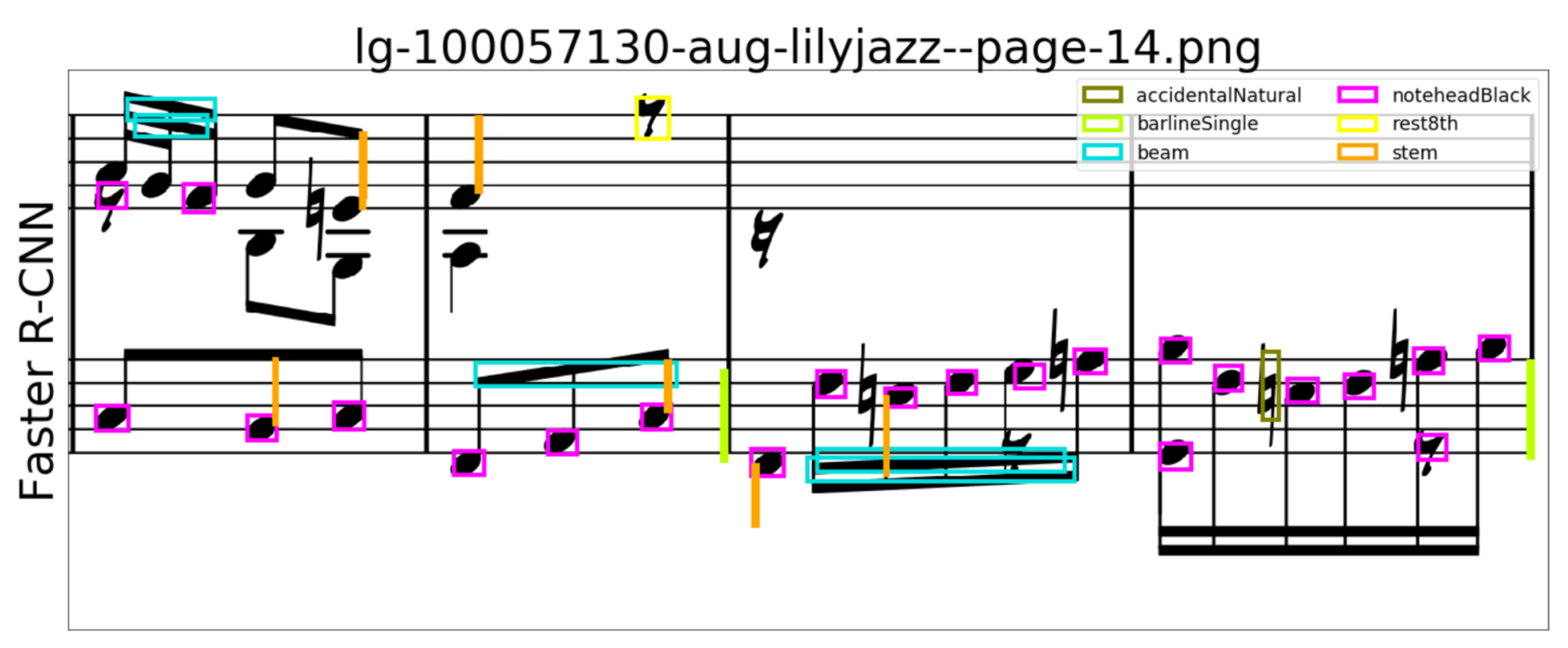
2.1. Object Detection-Based Approaches

In recent years, with the development of computer vision technology, the convolutional neural network (CNN) based on deep learning [6] technology has been increasingly applied to OCR and has achieved good results. During this period, a large number of object detection algorithms appeared, which were roughly divided into two categories: a one-stage detection algorithm and a two-stage detection algorithm.Typical one-stage detection models, such as YOLO [7,8,9] , SSD [10] and retina-net [11], do not require a regional proposal stage and directly generate the category probability and coordinate position values of objects. The final detection result can be obtained directly after a single detection, so it has a faster detection speed. On the contrary, two-stage detection algorithms, such as Fast R-CNN [12], Faster R-CNN [13], and R-FCN [14], have higher detection accuracy levels but slower speeds. Naturally, the exploration of CNN application in the OMR system is also in full swing.
Pacha et al. [15] proposed a baseline for general music object detection, which uses three different object detection models (Faster R-CNN, u-net [16], RetinaNet) for three different datasets (deepscores [17] as well as using MUSCIMA++ [18], capital) to detect notes. The test results of each model were given in terms of average precison.
Hajič jr. et al. [19] identified the notes in two stages. In the first stage, the input score image was segmented into a binary image using the semantic segmentation model, and the overall detection problem was decomposed into a set of binary pixel classification problems, and then the connected component detector was used to derive the final detection proposal. The experiment was aimed at the MUSCIMA++ dataset, showing the detection results of symbols in terms of f-scores.
Tuggener et al. [20] proposed the Deep Watershed Detector. They use ResNets [21] to predict dense energy maps that were used to predict the location, class, and bounding box of each symbol and could directly input the entire image without cropping each staff. They gave the final results for DeepScores and the MUSCIMA++ dataset. Their method was found to work well on small symbols, but there were problems such as inaccurate bounding boxes and undetectable rare classes.

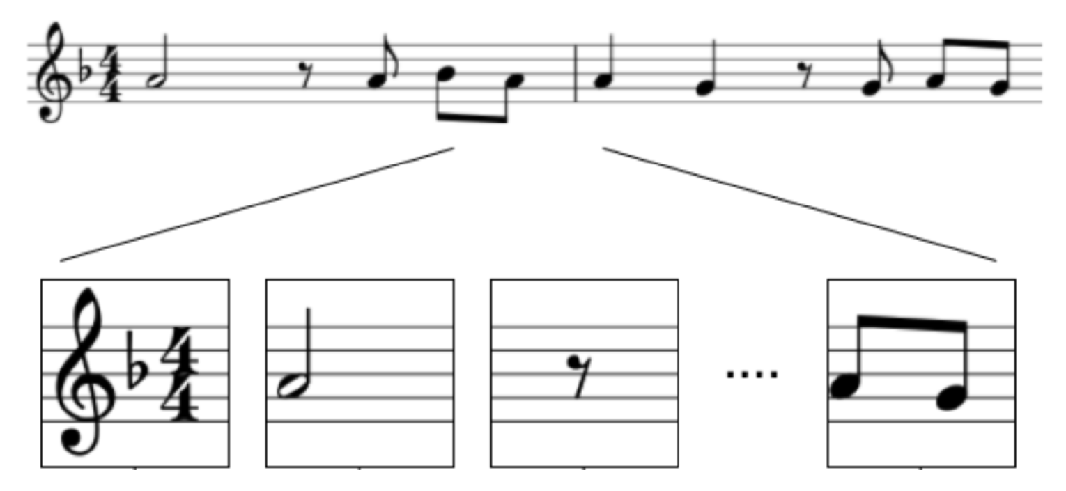
2.2. Sequential Recognition-Based Approaches

Another approach uses sequence-to-sequence architecture to translate OMR issues into translation problems. In the absence of context, instead of training a single segmentation symbol, the entire line of music is translated simultaneously. Those approaches mainly use convolutional neural networks (CNN) and recurrent neural networks (RNN), CNNs can learn local structures in images and combine them with useful features, so convolutional architecture has become a popular type of algorithm among various MIR-related tasks. RNN is critical in the sequence-to-sequence model and is often used in machine translation tasks [22,23].
Eelco van der Wel et al. [24] proposed the Convolutional Sequence-to-Sequence network, which uses CNN to encode the input image window into a series of vector representations. The encoder RNN then encodes the vector sequence into a fixed size representation and finally uses the RNN to decode the fixed size into an output tag sequence. The experiment yielded good results and demonstrated the pitch, time, and note accuracy. Calvo-Zaragoza et al. [25,26] also used a CNN to extract features from printed music scores and feed a Recurrent Neural Network. They used the Connectionist Temporal Classification (CTC) loss function to solve the problem of misalignment of different score image labels.

2.3. Summary

We observed some drawbacks in the above methods. After object detection-based approaches, additional steps are required to combine the symbols to obtain the note duration and pitch, and the detection accuracy of each symbol will affect the final result of duration and pitch. Sequential recognition-based approaches are only able to recognize monophonic music scores (no chords). In addition, they cannot identify dense music scores containing many accidentals, dynamics, or expression marks [27].
For all the above reasons, we propose an end-to-end music object detection model that can output symbol categories, symbol durations and pitches, as well as in monophonic music scores.

3. Dataset

The dataset in our experiment was derived from monophonic MusicXML scores from the MuseScore (https://musescore.org) sheet music archive. MuseScore is a type of free music notation software that also allows their users to upload their sheet music to their website and share it with others. We selected 10,000 MusicXML files to generate the dataset. Labels(category, bounding box, pitch, and duration) and score images were obtained by parsing each MusicMXL file. This study followed a fixed partitioning scheme where 70% of the dataset was used for training to learn the parameters of the neural model; 15% was used for verification and optimization of hyperparameters; and 15% was used for testing and calculating the final evaluation index.

3.1. Pre-Processing

Our corpus was composed of 10,000 MusicXML files (https://drive.google.com/open?id=1GCZ5r1s2-nDWUmGKPbTOQwDwhmwSgBc6). A dataset of images of score fragments and corresponding note labels was created from the corpus. The whole process was divided into three steps: Firstly, MusicXML and Scalable Vector Graphics (svg) were downloaded from MuseScore. Secondly, parse svg was used to get the bounding box of the symbol and convert svg was used to get the score image as well as the classes, duration, and pitch of notes from MusicXML. By combining known information, we were able to obtain score images, which are shown in Figure 1, and labels. The corresponding labels were represented with a pitch, duration, and bounding box vector. Note that the dataset we used was completely generated by MuseScore without any manual annotation.

3.1.1. Symbol Categories

The goal of our model is not to detect all symbols on the score, but to propose a new method of music object recognition (focusing on the recognition of note), we selected ten symbols (clefG, clefF, clefC, flat, natural, sharp, barline, timesig note, rest) as a key detection object because they account for 99% of all symbols. Then, get each category and its bounding box by parsing the svg file. Here, we do not need to detect hooks, dots, beams, stems. Please note that the rests of different durations belong to the same class, the notes of different durations and pitches belong to the same class, and the accidental sharp is the same as the sharp in the key signature. The representative symbols are depicted in Figure 2.

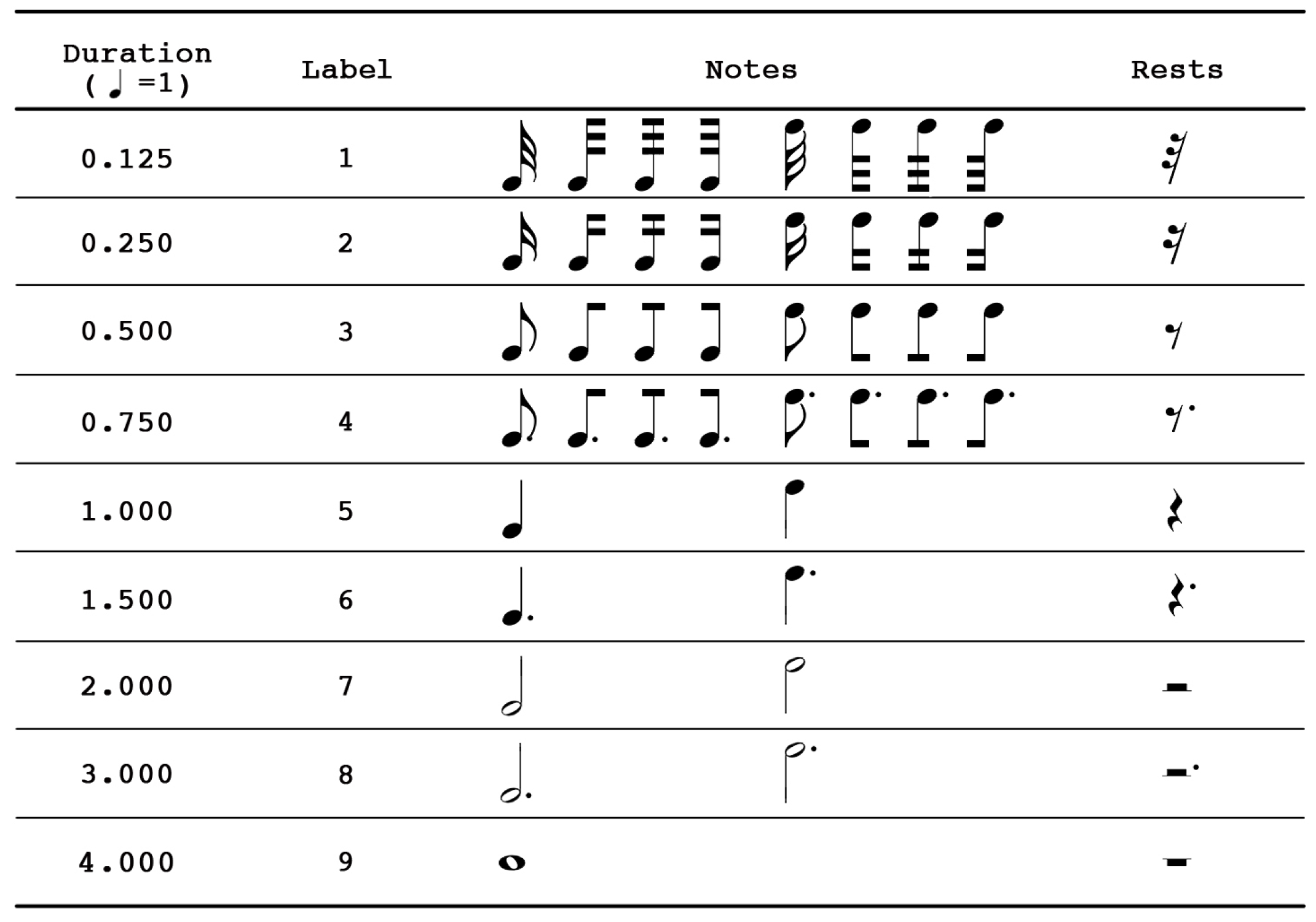
3.1.2. Symbol Duration
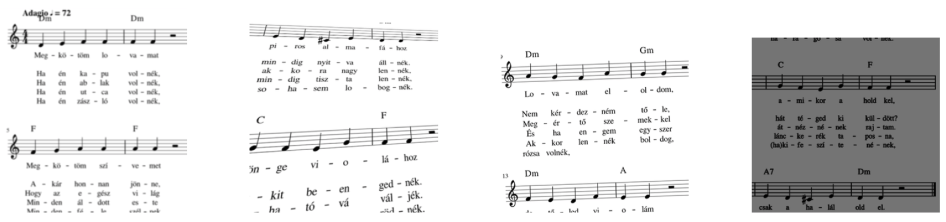
In the above method of classifying symbols, symbols of different duration belong to the same class. We needed to provide additional duration labels for notes and rests to distinguish between different symbols. Combining the relationship between the notehead, the beam, the dot, and the hook, we parsed the duration of the note and rest, and representative symbols are depicted in Figure 3.

3.1.3. Note Pitch

The pitch of a note is a vital piece of information in music score recognition. As shown in Figure 4, we used the relative position to represent the pitch, taking the fifth line of the staff line as the starting point. The vertical distance between the note and the starting point was recorded as the label, the number on the “2” side of the figure indicates the labels of pitch , in Figure 4, the label of the yellow note is 4, and the red note is 2 .

3.2. Image Augmentation

The images converted from svg contain no noise or variation in the musical symbols. This causes the neural network to learn stable symbol textures without generalization.In order to make the neural network model more robust, it was necessary to process the data on images to increase the diversity and variability. The method used in this article is shown below:
  • blur;
  • random crop;
  • Gaussian noise;
  • affine transformations;
  • elastic transformations;
  • hue, saturation, exposure shifts.
We used a total of six data processing methods, and we adjusted the composite parameters so that the score image was similar to the real-world score. For each training image, in order to make the notes larger in size, we randomly crop them into multiple images and stretched the cropped image. Then, two methods were randomly selected from the remaining five methods to process the data. Here, each cropped image had a 50% chance of being processd. In Figure 5, an example of these augmentations is shown.

4. Model

In this section, we introduce the end-to-end object detection model as applied to OMR tasks, translating music recognition tasks into detection and classification tasks. The bounding box of symbols was detected and the duration and pitch of symbols were classified.

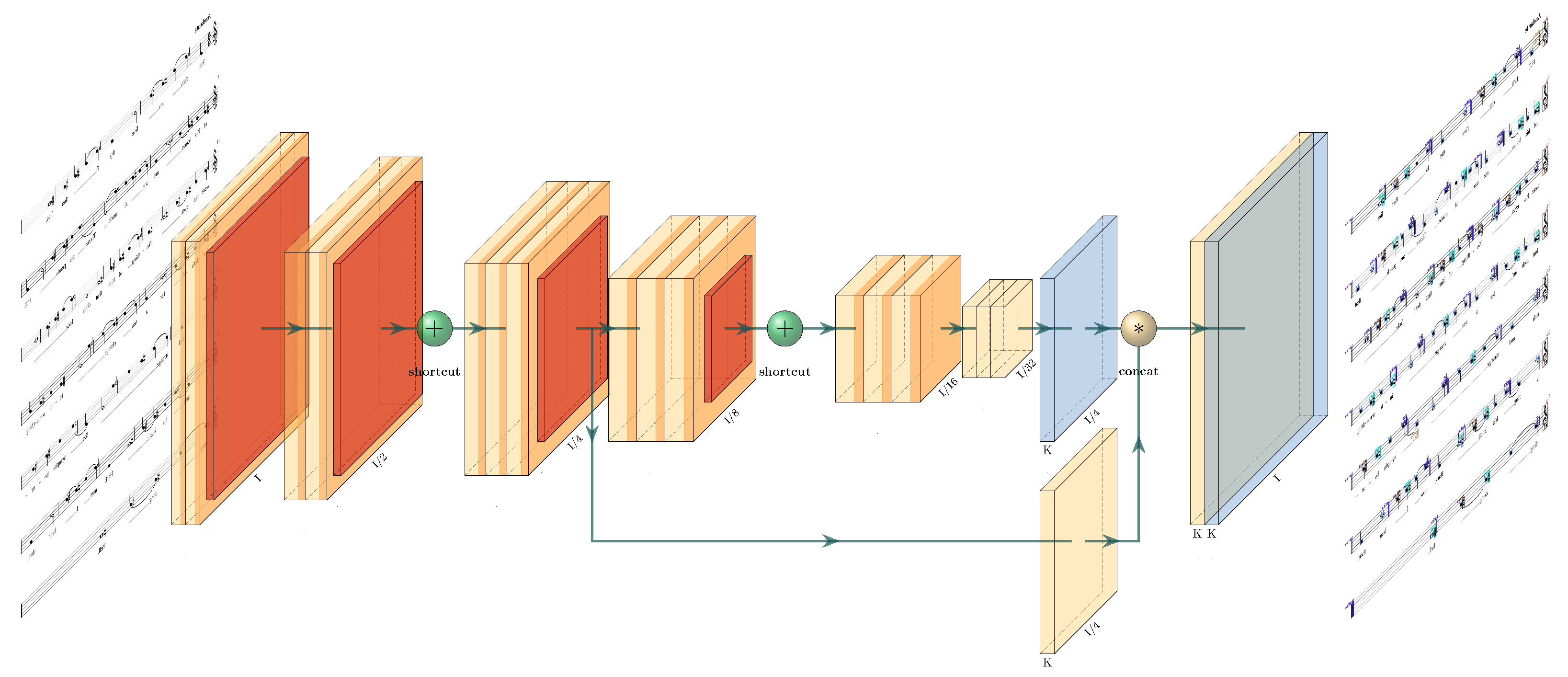
4.1. Network Architecture

The specific process of the our model is as follows: the score image is input into the convolutional neural network, and the feature map of the score image is extracted through a series of convolution, residual, and concatenated operations. Then, the symbol duration and pitch on the feature map are output, and the symbol bounding box is returned.
As shown in Figure 6, the input image size was 576 × 576 and the final feature size was 144 × 144. In order to make the symbols have a large enough receptive field, the model uses the darknet53 basic network in YOLO [9] to extract features. Considering that the feature of small objects will be lost after convolution, the darknet53 [9] basic network output feature map is upsampled 8 times and the feature map of the upper layer network is used for feature fusion to obtain more comprehensive feature information.The network structure of darknet53 is divided into five parts, namely conv1_x, conv2_x, conv3_x, conv4_x and conv5_x. conv1_x, conv2_x, conv3_x, conv4_x and conv5_x respectively comprise 1, 2, 8, 8, 6 building blocks, each building block consists of 2 convolution layers and a residual connection layer.
As shown in Figure 7, after the convolutional neural network outputs the feature map, an n-dimensional feature vector is generated based on each pixel point on the feature map, and the dimension n of the feature vector is 7 × (confidence + coordinates + symbols class + pitch category + duration category), that is, seven target candidate regions are generated in the n-dimensional feature vector. For each target candidate region, the sigmoid activation function is used to obtain the confidence of the target , the coordinates of the anchor boxes, the symbol class, the note pitch, and the symbol duration, so as to achieve multi-task training.
In the bounding box of the training dataset, k-means clustering is used to find the best width and height of the prior candidate box. In our work, a total of seven sizes of width and height were selected as the prior condition input. The use of k-means to generate candidate boxes will mean that the neural network model has better effects and is easier to learn.

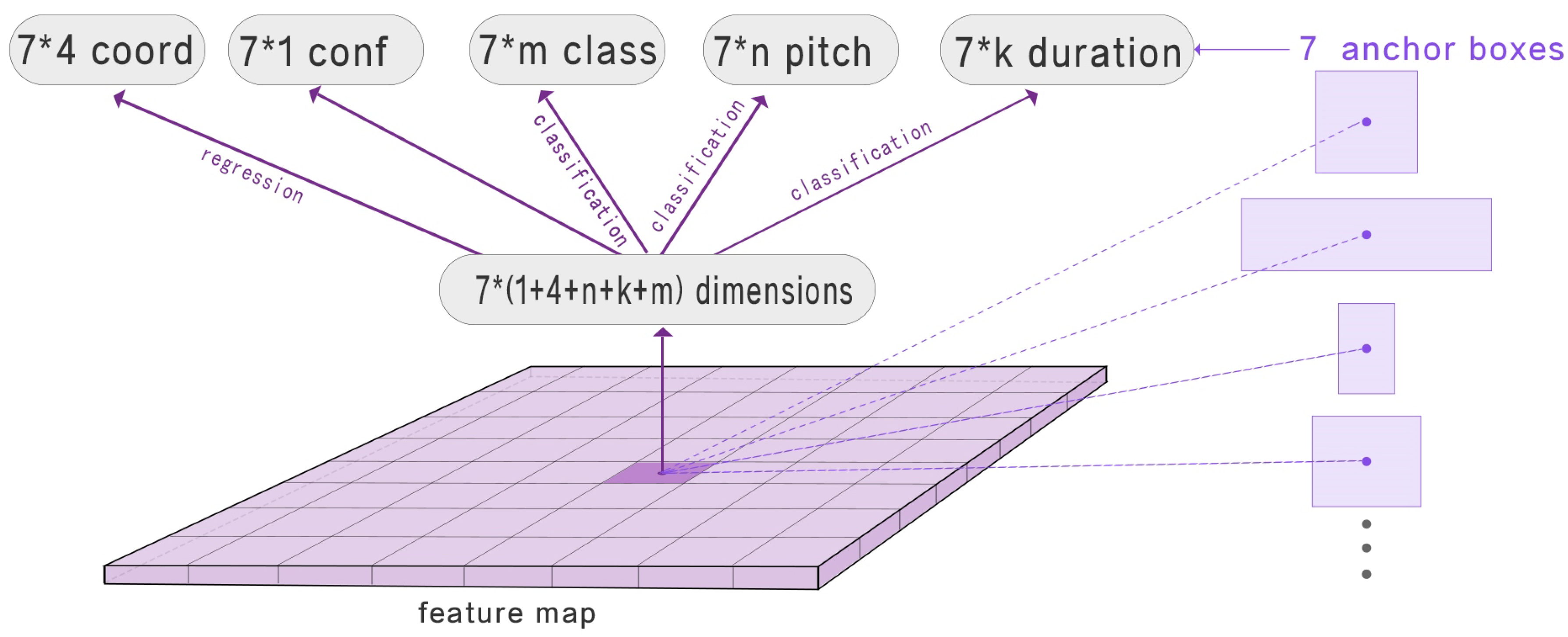
4.1.1. Class Prediction

We selected the 7× m-dimensional feature vector on the feature vector of the 7 × (1 + 4 + n + k + m) dimension generated by the pixel on the feature map, with a depth equal to the number of classes. The sigmoid activation function was applied to process the 7 × m features to generate the probability of each category. Finally, the binary cross entropy was used to calculate the loss function of the category l o s s c .

4.1.2. Predict Bounding Box

On the 7 × 4 feature vectors, 7 sets of offset coordinates ( t x , t y , t w , t h ) were generated by the sigmoid activation function, that is, 7 bounding boxes were generated at each pixel of the feature map. If the pixel of the cell is offset ( c x , c y ) from the upper left corner of the image, and the candidate box has prior information about the width and height ( p w , p h ), the predicted results are as follows:
b x = σ ( t x ) + c x b y = σ ( t y ) + c y b w = p w e t w b h = p h e t h .
The offset values are all between (0, 1), and the loss function of the offset is calculated using cross entropy: l o s s x , l o s s y , l o s s w , l o s s h .

4.1.3. Duration and Pitch

After predicting the bounding box of the symbol, we classified the duration and pitch of the symbol on the feature vectors 7 × n and 7 × k, where n and k are equal to the label’s length of duration and pitch. The probability of each classification was obtained through the sigmoid activation function. Then, l o s s d and l o s s p were calculated using cross entropy.

4.2. Losses

We wanted to jointly train all tasks; therefore, we defined l o s s t o t as
l o s s t o t = l o s s c + l o s s x + l o s s y + l o s s w + l o s s y + + l o s s d + l o s s p + l o s s c o n f
We predicted the confidence of each bounding box. First, we set the threshold of the area overlap between the predicted bounding box and the real bounding box to 0.6. In this model, if the predicted bounding box overlaps with the real regression box by more than any other predicted bounding box, this bounding box is set as the best match with a confidence of 1. If the overlap exceeds the threshold but is not within the optimal bounding box, the predicted bounding box is ignored, and the bounding box l o s s t o t is 0. At this time, l o s s t o t = l o s s c o n f . If the overlap is less than the threshold, the confidence of the bounding box is deemed to be 0. Finally, the l o s s c o n f of the confidence is calculated by binary cross entropy.
c o f i d e n c e = 1 , if best 0 , if overlap > threshold and not best i g n o r e , if overlap < threshold

5. Experiments and Results

5.1. Network Training

We trained an end-to-end network in order to achieve reasonable results. We only needed to provide the dataset generated by MuseScore and input it to the neural network. After the training stage, we were able to use the network to predict the desired result.
We rescaled the cropped image to a size of 576 × 576 pixels , which had two purposes: to perform efficient data augmentation and to process the input size of the image to give the target a larger receptive field. We set the batch size to 16 to reach the Nvidia Titian memory limit during training. Training was done using the Adam optimizer [28] with a learning rate of 0.005 and a decay rate of 0.995. A single Nvidia Titan Xp GPU was used for training and the model was trained in approximately 6 h.

5.2. Evaluation Metrics

For the test set, we calculated three evaluation metrics: the duration accuracy, pitch accuracy, and symbol average precision.
  • Pitch accuracy: the proportion of correctly predicted pitches.
  • Duration accuracy: the proportion of correctly predicted durations.
  • Symbol average precision [15]: the area under the precision–recall curve for all possible values of classes.
This was set to positive samples (PS) when the predicted durations of notes and rests were correct, otherwise it was set to negative samples (NS). The accuracy of the pitch was also calculated in this way:
a c c u r a r y = P S P S + N S

5.3. Results

The model tested a total of 1500 score images converted by MuseScore. The overall recognition results were a duration accuracy of 0.92 and a pitch accuracy of 0.96. Table 1 shows the average precision of each class. The results show that our model performs very well on score recognition tasks. The accuracy of duration and pitch was also higher than 0.9.
Figure 8 shows the detection effect of our network in the MuseScore test set. For the detected symbols, we drew the bounding box of the prediction, showing the duration and pitch of the symbol. In this simple score, the recognition results were almost entirely correct. Look carefully at the numbers marked on the notes and rests, for the two numbes on the notes, the first shows the duration of the note and the other represents the pitch, and the number on the rest indicates the duration. These data represent the duration and pitch of the model prediction, the mapping tabel corresponding to the labels of the duration and the pitch in the figure is shown in Section 3. We can directly obtain the final required duration and pitch of the symbol without detecting the hook, dot or beam.
At the same time, we randomly selected 2000 score images from Deepscores dataset, then we tested the score images and the test results were good, as shown in Figure 9. One problem is that there is a big gap between MuseScore and DeepScores’s labels, so we cannot quantitatively evaluate the results on DeepScores. Note that we used the MuseScore dataset for training without using any score images from DeepScores. Surprisingly, our training set consisted of monophonic scores, but our network was able to recognize polyphony and produced good results.We further applied the model to the natural scene, we took some music scores and used our model to recognize these images, as shown in Figure 10.

5.4. Comparison with Previous Approaches

Table 2 shows the current work for OMR. Similar to our work, E. van der Wel [24] applied the MuseScore dataset. In terms of recognition accuracy, our method has many advantages, with a mAP of 0.91, a duration accuracy of 0.92, and a pitch accuracy of 0.96.
Compared to sequential recognition-based approaches, we do not need to crop the image and directly input the entire image. As shown in Figure 11, they can only process one line of music score at a time.
Compared to object detection-based approaches, our work has many advantages. In References [15,20], related to music object detection, only symbols are detected, as shown in Figure 12 . If one wants to get the duration and pitch of the notes, they need extra steps, such as combining hook, beam, dot , and notehead to parse the duration; if one of the symbols is not detected, it will cause the final result to go wrong. We can directly output the duration and pitch of the note with a pitch accuracy of 0.96 and a duration accuracy of 0.92.

5.5. Discussion

From these results, we can conclude that our method works. There are some limitations to our system that are described below:
  • The ground truth does not provide the position of the clef on the stave. This means that a bass clef on the third or fourth staff lines are predicted as the same.
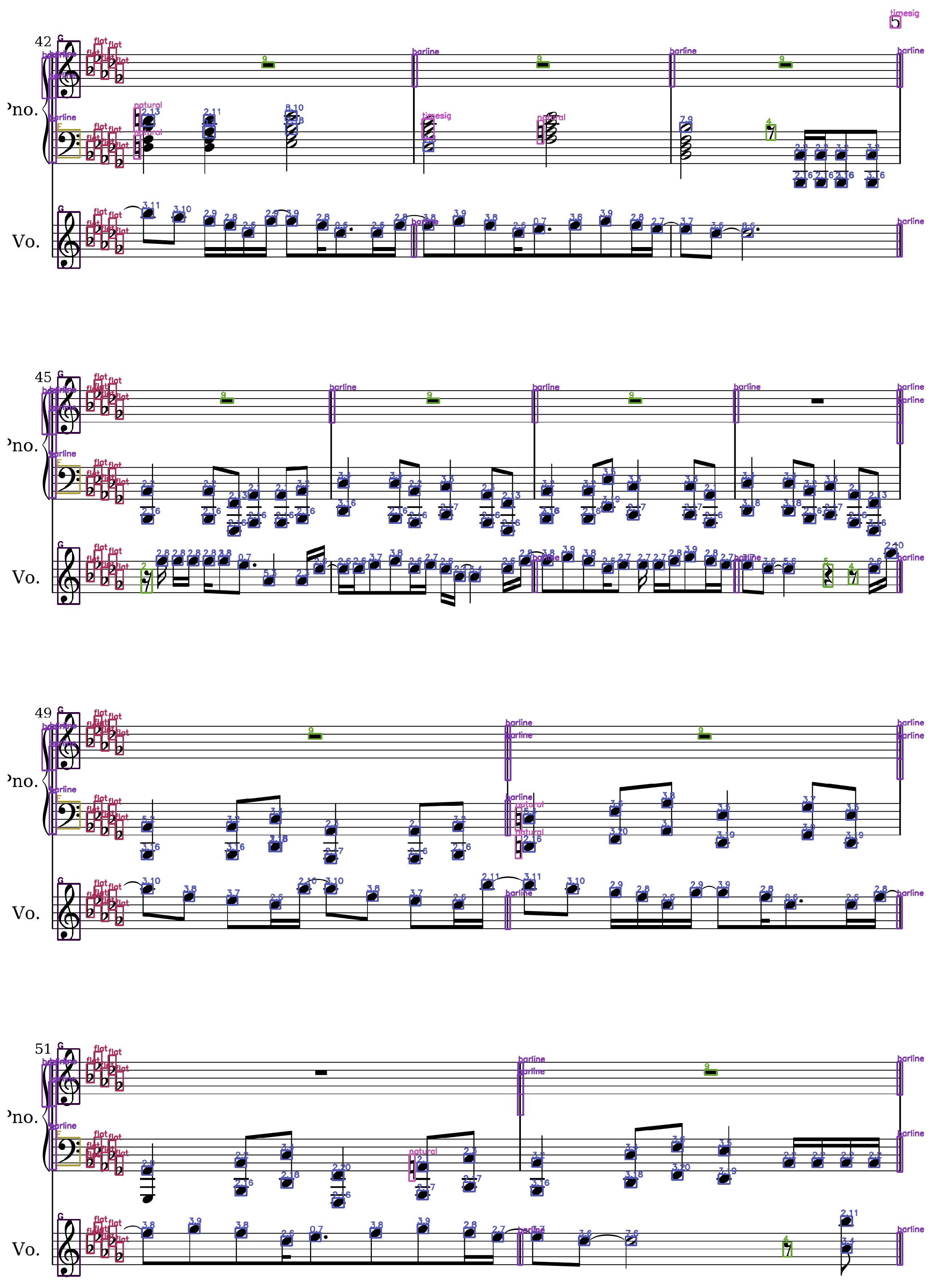
  • Our system generally struggles with rare classes, overlapping symbols, and dense symbols. We have calculated the distribution of symbols, the symbols that the model can recognize account for 99% and it is very challenging to detect these rare symbols (less than 1% of all symbols). For dense symbols (chords), our model will miss some notes.
  • As shown in Figure 3 and Figure 4, The duration of the symbols ranges from 0.125 to 4.000, and the pitch label of note ranges from −6 to 14. This means that the duration and pitch of the note can only be predicted within a certain range. If the range is exceeded, the pitch and duration of the symbols cannot be accurately predicted.

6. Conclusions and Future Work

In this work, we proposed a complete end-to-end printed score recognition model based on a deep convolutional neural network . The system only needs to input a complete score to be able to output the category, duration, and pitch of the symbols. The experimental results show that our approach produces state-of-the-art results when applied to MuseScore data. Our core is on the high efficiency of our model recognition (eliminating the cumbersome steps of semantic reconstruction, direct input of the whole picture, short time) and high accuracy. For general music scores, these categories contain most of the musical semantic information, and we have achieved good recognition (speed and accuracy) in these key categories, which proves the feasibility of our model. In future work, we plan to apply the system to handwritten scores and work on its performance.

Author Contributions

X.J. conceived of and designed the experiments. X.J. performed the experiments and analyzed the data. Y.G. contributed analysis tools. Z.H. and X.J. wrote the paper.

Funding

This research received no external funding.

Acknowledgments

The authors wish to thank the anonymous reviewers for their valuable suggestions.

Conflicts of Interest

The authors declare no conflict of interest.

Abbreviations

MIDIMusical Instrument Digital Interface
R-CNNRegion-based Convolutional Neural Network
SSDSingle Shot Detector
YOLOYou Only Look Once
mAPMean Average Precision
CNNConvolutional Neural Network
RNNRecurrent Neural Network
CTCConnectionist Temporal Classification
GPUGraphical Processing Units
AdamA Method for Stochastic Optimization

References

  1. Casey, M.; Veltkamp, R.; Goto, M.; Leman, M.; Rhodes, C.; Slaney, M. Content-Based Music Information Retrieval: Current Directions and Future Challenges. Proc. IEEE 2008, 96, 668–696. [Google Scholar] [CrossRef] [Green Version]
  2. Roland, P. The Music Encoding Initiative (MEI). In Proceedings of the First International Conference on Musical Applications Using XML, Milan, Italy, 19–20 September 2002; pp. 55–59. [Google Scholar]
  3. Good, M.; Actor, G. Using MusicXML for file interchange. In Proceedings of the Third International Conference on WEB Delivering of Music, Leeds, UK, 15–17 September 2003; p. 153. [Google Scholar] [CrossRef]
  4. Bainbridge, D.; Bell, T. The challenge of optical music recognition. Comput. Humanit. 2001, 35, 95–121. [Google Scholar] [CrossRef]
  5. Rebelo, A.; Fujinaga, I.; Paszkiewicz, F.; Marcal, A.R.S.; Guedes, C.; Cardoso, J.S. Optical music recognition: State-of-the-art and open issues. Int. J. Multimed. Inf. Retr. 2012, 1, 173–190. [Google Scholar] [CrossRef]
  6. LeCun, Y.; Bengio, Y.; Hinton, G. Deep learning. Nature 2015, 521, 436–444. [Google Scholar] [CrossRef] [PubMed]
  7. Redmon, J.; Divvala, S.; Girshick, R.; Farhadi, A. You Only Look Once: Unified, Real-Time Object Detection. arXiv 2015, arXiv:1506.02640. [Google Scholar]
  8. Redmon, J.; Farhadi, A. YOLO9000: Better, Faster, Stronger. arXiv 2016, arXiv:1612.08242. [Google Scholar]
  9. Redmon, J.; Farhadi, A. YOLOv3: An Incremental Improvement. arXiv 2018, arXiv:1804.02767. [Google Scholar]
  10. Liu, W.; Anguelov, D.; Erhan, D.; Szegedy, C.; Reed, S.; Fu, C.Y.; Berg, A.C. SSD: Single Shot MultiBox Detector. In European Conference on Computer Vision; Springer: Cham, Switzerland, 2016; pp. 21–37. [Google Scholar] [Green Version]
  11. Lin, T.Y.; Goyal, P.; Girshick, R.; He, K.; Dollár, P. Focal Loss for Dense Object Detection. arXiv 2017, arXiv:1708.02002. [Google Scholar]
  12. Girshick, R. Fast R-CNN. arXiv 2015, arXiv:1504.08083. [Google Scholar]
  13. Ren, S.; He, K.; Girshick, R.; Sun, J. Faster R-CNN: Towards Real-Time Object Detection with Region Proposal Networks. arXiv 2015, arXiv:1506.01497. [Google Scholar] [CrossRef] [PubMed]
  14. Dai, J.; Li, Y.; He, K.; Sun, J. R-FCN: Object Detection via Region-based Fully Convolutional Networks. arXiv 2016, arXiv:1605.06409. [Google Scholar]
  15. Pacha, A.; Hajič, J.; Calvo-Zaragoza, J. A Baseline for General Music Object Detection with Deep Learning. Appl. Sci. 2018, 8, 1488. [Google Scholar] [CrossRef]
  16. Ronneberger, O.; Fischer, P.; Brox, T. U-Net: Convolutional Networks for Biomedical Image Segmentation. arXiv 2015, arXiv:1505.04597. [Google Scholar]
  17. Tuggener, L.; Elezi, I.; Schmidhuber, J.; Pelillo, M.; Stadelmann, T. DeepScores—A Dataset for Segmentation, Detection and Classification of Tiny Objects. arXiv 2018, arXiv:1804.00525. [Google Scholar]
  18. Hajič, J.; Pecina, P. The MUSCIMA++ Dataset for Handwritten Optical Music Recognition. In Proceedings of the 2017 14th IAPR International Conference on Document Analysis and Recognition (ICDAR), Kyoto, Japan, 10 November 2017; pp. 39–46. [Google Scholar] [CrossRef]
  19. Hajič, J., Jr.; Dorfer, M.; Widmer, G.; Pecina, P. Towards Full-Pipeline Handwritten OMR with Musical Symbol Detection by U-Nets. In Proceedings of the 19th International Society for Music Information Retrieval Conference, Paris, France, 23–27 September 2018; pp. 23–27. [Google Scholar]
  20. Tuggener, L.; Elezi, I.; Schmidhuber, J.; Stadelmann, T. Deep Watershed Detector for Music Object Recognition. arXiv 2018, arXiv:1805.10548. [Google Scholar]
  21. He, K.; Zhang, X.; Ren, S.; Sun, J. Deep Residual Learning for Image Recognition. arXiv 2015, arXiv:1512.03385. [Google Scholar]
  22. Cho, K.; van Merrienboer, B.; Gulcehre, C.; Bahdanau, D.; Bougares, F.; Schwenk, H.; Bengio, Y. Learning Phrase Representations using RNN Encoder-Decoder for Statistical Machine Translation. arXiv 2014, arXiv:1406.1078. [Google Scholar]
  23. Sutskever, I.; Vinyals, O.; Le, Q.V. Sequence to Sequence Learning with Neural Networks. In Advances in Neural Information Processing Systems 27; Ghahramani, Z., Welling, M., Cortes, C., Lawrence, N.D., Weinberger, K.Q., Eds.; Curran Associates, Inc.: Nice, France, 2014; pp. 3104–3112. [Google Scholar]
  24. van der Wel, E.; Ullrich, K. Optical Music Recognition with Convolutional Sequence-to-Sequence Models. arXiv 2017, arXiv:1707.04877. [Google Scholar]
  25. Calvo-Zaragoza, J.; Valero-Mas, J.J.; Pertusa, A. END-TO-END OPTICAL MUSIC RECOGNITION USING NEURAL NETWORKS. In Proceedings of the 18th International Society for Music Information Retrieval Conference, Suzhou, China, 472–477 Octorber 2017; pp. 23–27. [Google Scholar]
  26. Calvo-Zaragoza, J.; Rizo, D. End-to-End Neural Optical Music Recognition of Monophonic Scores. Appl. Sci. 2018, 8, 606. [Google Scholar] [CrossRef]
  27. Baró, A.; Riba, P.; Calvo-Zaragoza, J.; Fornés, A. From Optical Music Recognition to Handwritten Music Recognition: A baseline. Pattern Recognit. Lett. 2019, 123, 1–8. [Google Scholar] [CrossRef] [Green Version]
  28. Kingma, D.P.; Ba, J. Adam: A Method for Stochastic Optimization. arXiv 2014, arXiv:1412.6980. [Google Scholar]
Figure 1. Samples of notations from MuseScore.
Applsci 09 02645 g001
Figure 2. The classes of symbols from MuseScore used in our work. These symbols are depicted without considering their pitch and duration.
Applsci 09 02645 g002
Figure 3. Encoding the duration into discrete categories. Nine kinds of durations were used in our work, and each duration corresponded to a different note. The duration was encoded as a label between 1 and 9.
Applsci 09 02645 g003
Figure 4. Encoding of the pitch with a vertical distance. The numbers in the figure represent the labels of the pitch. The label of the red headnote is 2 , and the label of the yellow headnote is 4.
Applsci 09 02645 g004
Figure 5. The whole score was cropped and four images were generated. The first image was Gaussian blurred; the second image was affine transformed and rotated 5 degrees to the left; the next image was elastically transformed, and the last image used color transform to simulate the effects of illumination on the image.
Applsci 09 02645 g005
Figure 6. A diagram of the proposed end-to-end object detection model. Darknet53 is applied as the backbone network, the features are extracted using a convolutional neural network, and then upsampling and feature fusion are conducted to get the final feature map.
Applsci 09 02645 g006
Figure 7. The last layer of the network: the symbol class, pitch, and duration are classified, and the coordinates of the symbol are obtained by regression.
Applsci 09 02645 g007
Figure 8. Detection results sample: MuseScore.
Applsci 09 02645 g008
Figure 9. Detection results sample: DeepScores.
Applsci 09 02645 g009
Figure 10. Detection results sample: image taken from a mobile phone.
Applsci 09 02645 g010
Figure 11. Image from Eelco van der Wel et al. [24].
Applsci 09 02645 g011
Figure 12. Detection results on DeepScores:image from Pacha et al. [15].
Applsci 09 02645 g012
Table 1. Results in terms of Average Precision(AP)(%) with respect to the dataset (MuseScore).
ClassSharpFlatNaturalclefGclefFclefCBarlineTimesigNoteRest
AP0.960.930.920.980.960.860.90.820.940.92
Table 2. Comparison of our results with current methods.
MethodDatasetResult
Eelco van der Wel [24]printed scoreaccuracy
MuseScore0.81 (pitch)0.80 (note)0.94 (duration)
oursprinted scoreaccuracy and mean average precision
MuseScore0.96 (pitch)0.91 (symbols)0.92 (duration)

