Parallel Hierarchical Genetic Algorithm for Scattered Data Fitting through B-Splines

 , ,
, ,  ,
,  and
and
Abstract
1. Introduction
2. Related Work
3. Background
3.1. Curve Fitting with B-Spline Curves
3.2. Hierarchical Genetic Algorithms
4. B-Spline Curve Fitting Using PHGA
4.1. Chromosome Encoding
4.2. Fitness Function
4.2.1. Akaike’s Information Criterion
4.2.2. Knot Structure Function
4.3. Selection Scheme
4.4. Genetic Operators
4.4.1. Crossover Operator
4.4.2. Mutation Operator
4.5. Parallel Hierarchical Genetic Algorithm
Migration Operator
5. Simulation Results
5.1. Experimental Set
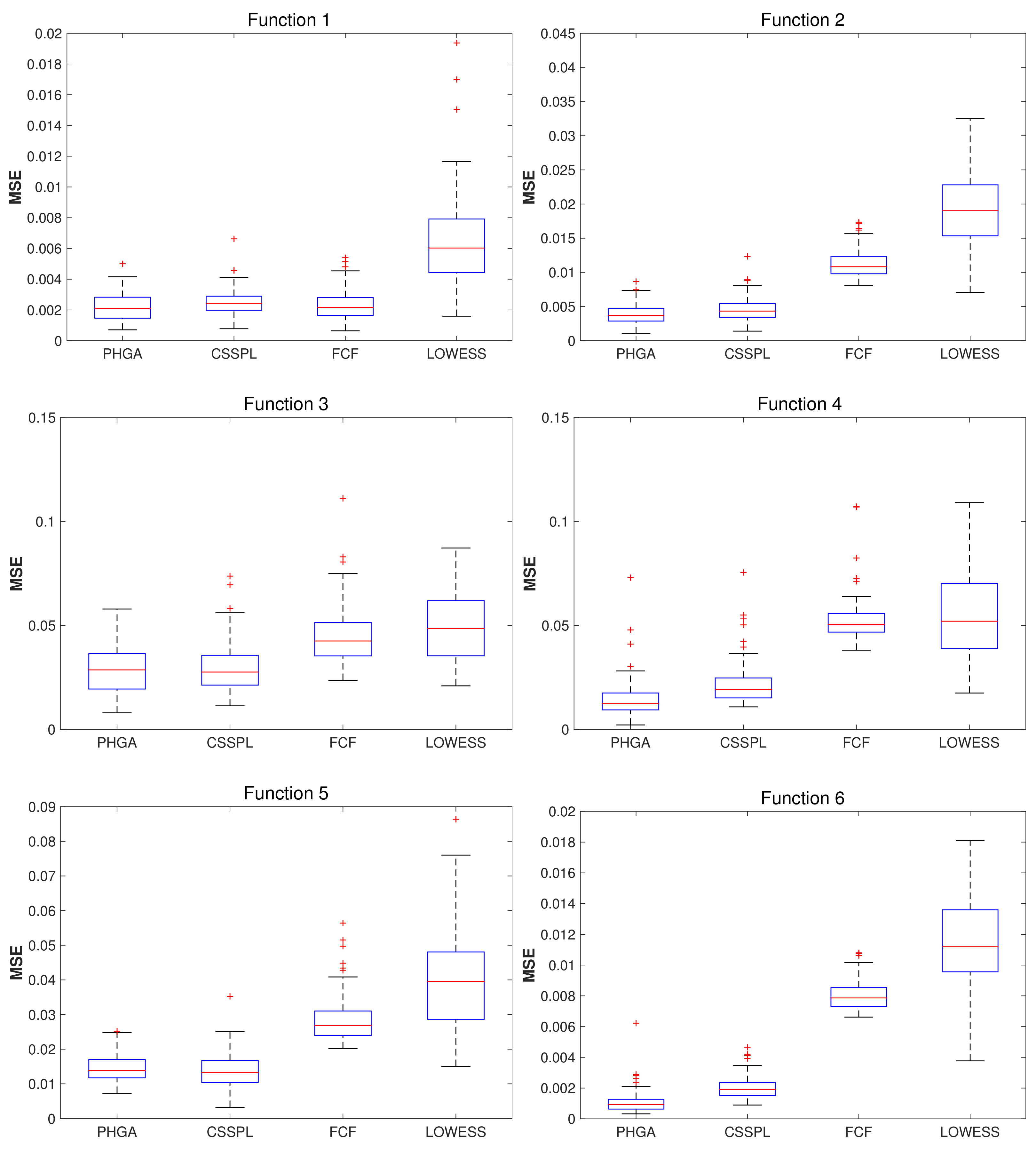
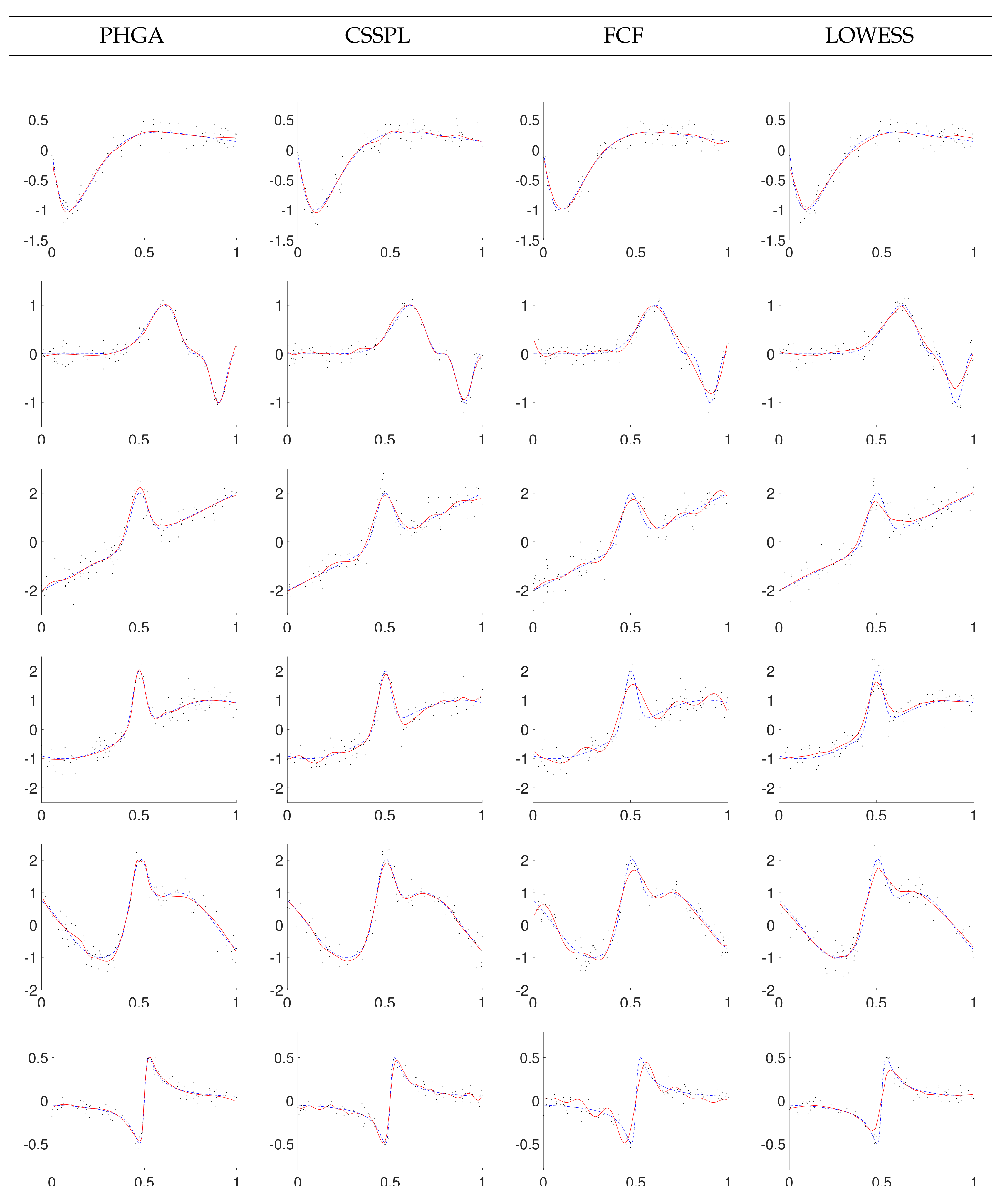
5.2. Results
6. Conclusions
Author Contributions
Funding
Conflicts of Interest
References
- Wendland, H. Scattered Data Approximation; Cambridge University Press: Cambridge, UK, 2004. [Google Scholar]
- Johnson, M.J.; Shen, Z.; Xu, Y. Scattered data reconstruction by regularization in B-spline and associated wavelet spaces. J. Approx. Theory 2009, 159, 197–223. [Google Scholar] [CrossRef][Green Version]
- Lee, S.; Wolberg, G.; Shin, S.Y. Scattered Data Interpolation with Multilevel B-Splines. IEEE Trans. Vis. Comput. Graph. 1997, 3, 228–244. [Google Scholar] [CrossRef]
- Davydov, O.; Schumaker, L.L. Scattered Data Fitting on Surfaces Using Projected Powell-Sabin Splines. In Proceedings of the Mathematics of Surfaces XII: 12th IMA International Conference, Sheffield, UK, 4–6 September 2007; Martin, R., Sabin, M., Winkler, J., Eds.; Springer: Berlin/Heidelberg, Germany, 2007; pp. 138–153. [Google Scholar]
- Tjahjowidodo, T.; Dung, V.; Han, M. A fast non-uniform knots placement method for B-spline fitting. In Proceedings of the 2015 IEEE International Conference on Advanced Intelligent Mechatronics (AIM), Busan, Korea, 7–11 July 2015; pp. 1490–1495. [Google Scholar]
- Li, W.; Xu, S.; Zhao, G.; Goh, L.P. A Heuristic Knot Placement Algorithm for B-Spline Curve Approximation. Comput.-Aided Des. Appl. 2004, 1, 727–732. [Google Scholar] [CrossRef]
- Holland, J.H. Adaptation in Natural and Artificial Systems: An Introductory Analysis with Applications to Biology, Control and Artificial Intelligence; The MIT Press: Cambridge, MA, USA, 1992. [Google Scholar]
- Luque, G.; Alba, E. Parallel Models for Genetic Algorithms. In Parallel Genetic Algorithms: Theory and Real World Applications; Springer: Berlin/Heidelberg, Germany, 2011; pp. 15–30. [Google Scholar]
- Iske, A. Scattered data approximation by positive definite kernel functions. Rend. Semin. Mat. Univ. Politec. Torino 2011, 69, 217–246. [Google Scholar]
- Ardjmand, E.; Young, W.A.; Weckman, G.R.; Bajgiran, O.S.; Aminipour, B.; Park, N. Applying genetic algorithm to a new bi-objective stochastic model for transportation, location, and allocation of hazardous materials. Expert Syst. Appl. 2016, 51, 49–58. [Google Scholar] [CrossRef]
- Shahvari, O.; Logendran, R. Hybrid flow shop batching and scheduling with a bi-criteria objective. Int. J. Prod. Econ. 2016, 179, 239–258. [Google Scholar] [CrossRef]
- Shahvari, O.; Logendran, R. An Enhanced tabu search algorithm to minimize a bi-criteria objective in batching and scheduling problems on unrelated-parallel machines with desired lower bounds on batch sizes. Comput. Oper. Res. 2017, 77, 154–176. [Google Scholar] [CrossRef]
- Shahvari, O.; Salmasib, N.; Logendranc, R.; Abbasid, B. An efficient tabu search algorithm for flexible flow shop sequence-dependent group scheduling problems. Int. J. Prod. Res. 2012, 50, 4237–4254. [Google Scholar] [CrossRef]
- Glover, F. Tabu search—Part I. ORSA J. Comput. 1989, 1, 190–206. [Google Scholar] [CrossRef]
- Piniganti, L. A Survey of Tabu Search in Combinatorial Optimization. Master’s Thesis, University of Nevada, Las Vegas, NV, USA, 2014. [Google Scholar]
- Glover, F. Tabu Search for nonlinear and parametric optimization (with links to genetic algorithms). Discret. Appl. Math. 1994, 49, 231–255. [Google Scholar] [CrossRef]
- Garcia-Capulin, C.H.; Cuevas, F.J.; Trejo-Caballero, G.; Rostro-Gonzalez, H. A hierarchical genetic algorithm approach for curve fitting with B-splines. Genet. Program. Evol. Mach. 2015, 16, 151–166. [Google Scholar] [CrossRef]
- Szwed, P.; Chmiel, W.; Kadłuczka, P. OpenCL Implementation of PSO Algorithm for the Quadratic Assignment Problem. In Artificial Intelligence and Soft Computing; Rutkowski, L., Korytkowski, M., Scherer, R., Tadeusiewicz, R., Zadeh, L.A., Zurada, J.M., Eds.; Springer International Publishing: Cham, Switzerlands, 2015; pp. 223–234. [Google Scholar]
- Yoshimura, M.; Izui, K. Hierarchical Parallel Processes of Genetic Algorithms for Design Optimization of Large-Scale Products. J. Mech. Des. 2004, 126, 217–224. [Google Scholar] [CrossRef]
- Lim, D.; Ong, Y.S.; Jin, Y.; Sendhoff, B.; Lee, B.S. Efficient Hierarchical Parallel Genetic Algorithms using Grid computing. Future Gener. Comput. Syst. 2007, 23, 658–670. [Google Scholar] [CrossRef]
- Plichta, A.; Gaciarz, T.; Baranowski, B.; Szominski, S. Implementation of the genetic algorithm by means of CUDA technology involved in travelling salesman problem. In Proceedings of the 28th European Conference on Modelling and Simulation (ECMS), Brescia, Italy, 27–30 May 2014. [Google Scholar]
- Bhardwaj, G.; Pandey, M. Parallel Implementation of Travelling Salesman Problem using Ant Colony Optimization. Int. J. Comput. Appl. Technol. Res. 2014, 3, 385–389. [Google Scholar] [CrossRef]
- Zhou, Y.; He, F.; Hou, N.; Qiu, Y. Parallel ant colony optimization on multi-core SIMD CPUs. Future Gener. Comput. Syst. 2018, 79, 473–487. [Google Scholar] [CrossRef]
- Cai, P.; Cai, Y.; Chandrasekaran, I.; Zheng, J. Parallel genetic algorithm based automatic path planning for crane lifting in complex environments. Autom. Constr. 2016, 62, 133–147. [Google Scholar] [CrossRef]
- Brookhouse, J.; Otero, F.E.B.; Kampouridis, M. Working with OpenCL to speed up a genetic programming financial forecasting algorithm: Initial results. In Proceedings of the Companion Publication of the 2014 Annual Conference on Genetic and Evolutionary Computation (GECCO Comp ’14), Vancouver, BC, Canada, 12–16 July 2014. [Google Scholar]
- Augusto, D.A.; Barbosa, H.J.C. Accelerated parallel genetic programming tree evaluation with OpenCL. J. Parallel Distrib. Comput. 2013, 73, 86–100. [Google Scholar] [CrossRef]
- Huang, C.S.; Huang, Y.C.; Lai, P.J. Modified genetic algorithms for solving fuzzy flow shop scheduling problems and their implementation with CUDA. Expert Syst. Appl. 2012, 39, 4999–5005. [Google Scholar] [CrossRef]
- Rocha, I.; Parente, E.; Melo, A. A hybrid shared/distributed memory parallel genetic algorithm for optimization of laminate composites. Compos. Struct. 2014, 107, 288–297. [Google Scholar] [CrossRef]
- Omkar, S.; Venkatesh, A.; Mudigere, M. MPI-based parallel synchronous vector evaluated particle swarm optimization for multi-objective design optimization of composite structures. Eng. Appl. Artif. Intell. 2012, 25, 1611–1627. [Google Scholar] [CrossRef]
- Walker, R.L. Search engine case study: Searching the web using genetic programming and MPI. Parallel Comput. 2001, 27, 71–89. [Google Scholar] [CrossRef]
- Imbernón, B.; Prades, J.; Giménez, D.; Cecilia, J.M.; Silla, F. Enhancing large-scale docking simulation on heterogeneous systems: An MPI vs. rCUDA study. Future Gener. Comput. Syst. 2018, 79, 26–37. [Google Scholar] [CrossRef]
- Li, D.; Li, K.; Liang, J.; Ouyang, A. A hybrid particle swarm optimization algorithm for load balancing of MDS on heterogeneous computing systems. Neurocomputing 2019, 330, 380–393. [Google Scholar] [CrossRef]
- Spanos, A. Curve Fitting, the Reliability of Inductive Inference, and the Error-Statistical Approach. Philos. Sci. 2007, 74, 1046–1066. [Google Scholar] [CrossRef]
- Boor, C.D. A Practical Guide to Splines; Applied Mathematical Sciences; Springer: New York, NY, USA, 2001. [Google Scholar]
- Piegl, L.; Tiller, W. The NURBS Book; Monographs in Visual Communication; Springer: Berlin/Heidelberg, Germany, 1997. [Google Scholar]
- Jong, E.D.D.; Watson, R.A.; Thierens, D. On the Complexity of Hierarchical Problem Solving. In Proceedings of the 7th Annual Conference on Genetic and Evolutionary Computation (GECCO ’05), Washington, DC, USA, 25–29 June 2005; ACM: New York, NY, USA, 2005; pp. 1201–1208. [Google Scholar]
- Man, K.F.; Tang, K.S.; Kwong, S. Genetic Algorithms: Concepts and Designs, 2nd ed.; Advanced Textbooks in Control and Signal Processing; Springer: London, UK, 1999. [Google Scholar]
- Jong, E.D.D.; Thierens, D.; Watson, R.A. Hierarchical Genetic Algorithms. In Proceedings of the Parallel Problem Solving from Nature—PPSN VIII: 8th International Conference, Birmingham, UK, 18–22 September 2004; Springer: Berlin/Heidelberg, Germany, 2004; pp. 232–241. [Google Scholar]
- Deb, K. Multi-Objective Optimization Using Evolutionary Algorithms; John Wiley & Sons, Inc.: New York, NY, USA, 2001. [Google Scholar]
- Akaike, H. A new look at the statistical model identification. IEEE Trans. Autom. Control 1974, 19, 716–723. [Google Scholar] [CrossRef]
- Lee, T.C.M. Regression spline smoothing using the minimum description length principle. Stat. Probab. Lett. 2000, 48, 71–82. [Google Scholar] [CrossRef]
- Mitchell, M. An Introduction to Genetic Algorithms; A Bradford Book; MIT Press: Cambridge, MA, USA, 1998. [Google Scholar]
- Sivanandam, S.; Deepa, S. Introduction to Genetic Algorithms; Springer: Berlin/Heidelberg, Germany, 2008. [Google Scholar]
- Deb, K.; Agrawal, R.B. Simulated Binary Crossover for Continuous Search Space. Complex Syst. 1995, 9, 115–148. [Google Scholar]
- Alba, E.; Troya, J.M. A Survey of Parallel Distributed Genetic Algorithms. Complex 1999, 4, 31–52. [Google Scholar] [CrossRef]
- Belding, T.C. The Distributed Genetic Algorithm Revisited. In Proceedings of the 6th International Conference on Genetic Algorithms; Morgan Kaufmann Publishers Inc.: San Francisco, CA, USA, 1995; pp. 114–121. [Google Scholar]
- Rucinski, M.; Izzo, D.; Biscani, F. On the impact of the migration topology on the Island Model. Parallel Computing. 2010, 36, 555–571. [Google Scholar] [CrossRef]
- Dimatteo, I.; Genovese, C.R.; Kass, R.E. Bayesian curve-fitting with free-knot splines. Biometrika 2001, 88, 1055–1071. [Google Scholar] [CrossRef]
- Denison, D.; Mallick, B.; Smith, A. Automatic Bayesian Curve Fitting. J. R. Stat. Soc. Ser. B (Stat. Methodol.) 1998, 60, 333–350. [Google Scholar] [CrossRef]
- Pittman, J. Adaptive Splines and Genetic Algorithms. J. Comput. Graph. Stat. 2002, 11, 615–638. [Google Scholar] [CrossRef]
- Gálvez, A.; Iglesias, A. Efficient particle swarm optimization approach for data fitting with free knot-splines. Comput.-Aided Des. 2011, 43, 1683–1692. [Google Scholar] [CrossRef]


| Problem | Technique | Platform | Technology | Reference |
|---|---|---|---|---|
| Travelling salesman | Genetic Algorithms | GPU | CUDA | [21] |
| Travelling salesman | Ant Colony | GPU, CPU | OpenCL | [22] |
| Traveling salesman problem | Ant Colony | GPU, CPU | OpenCL | [23] |
| Financial Forecasting Algorithm | Genetic Programming | GPU, CPU | OpenCL | [25] |
| Automatic path planning | Genetic Algorithm | GPU | CUDA | [24] |
| Tree evaluation | Genetic Algorithms | GPU, CPU | OpenCL | [26] |
| Flow shop scheduling | Genetic Algorithms | GPU | CUDA | [27] |
| Optimization of composite laminate plates | Genetic Algorithms | CPU | OpenMP, MPI | [28] |
| Optimization of composite laminate plates | Particle Swarm, Genetic Algorithms | CPU | MPI | [29] |
| Search engine | Genetic Programming | CPU | MPI | [30] |
| Quadratic Assignment Problem | Particle Swarm | GPU | OpenCL | [18] |
| Molecular docking | Genetic Algorithms | GPU | MPI, OpenMP, CUDA, OpenMP | [31] |
| Molecular dynamics simulation | Particle Swarm, Genetic Algorithms | GPU, CPU | OpenMP, CUDA | [32] |
| Number | Function | Domain |
|---|---|---|
| 1 | with | |
| 2 | ||
| 3 | ||
| 4 | ||
| 5 | ||
| 6 |
| Parameter | Value |
|---|---|
| Island population size | 200 |
| Number of Islands | 10 |
| Size of elite population | 10 |
| Crossover probability | 0.85 |
| Mutation probability | 0.01 |
| Migration size | 10 |
| Migration interval | 200 epoch |
| Migration policy | Best Replace worst |
| Migration topology | Ring |
| Test | Method | SNR = 1 | SNR = 2 | SNR = 3 |
|---|---|---|---|---|
| 1 | CSSPL | |||
| FCF | ||||
| LOWESS | ||||
| PHGA | ||||
| 2 | CSSPL | |||
| FCF | ||||
| LOWESS | ||||
| PHGA | ||||
| 3 | CSSPL | |||
| FCF | ||||
| LOWESS | ||||
| PHGA | ||||
| 4 | CSSPL | |||
| FCF | ||||
| LOWESS | ||||
| PHGA | ||||
| 5 | CSSPL | |||
| FCF | ||||
| LOWESS | ||||
| PHGA | ||||
| 6 | CSSPL | |||
| FCF | ||||
| LOWESS | ||||
| PHGA |
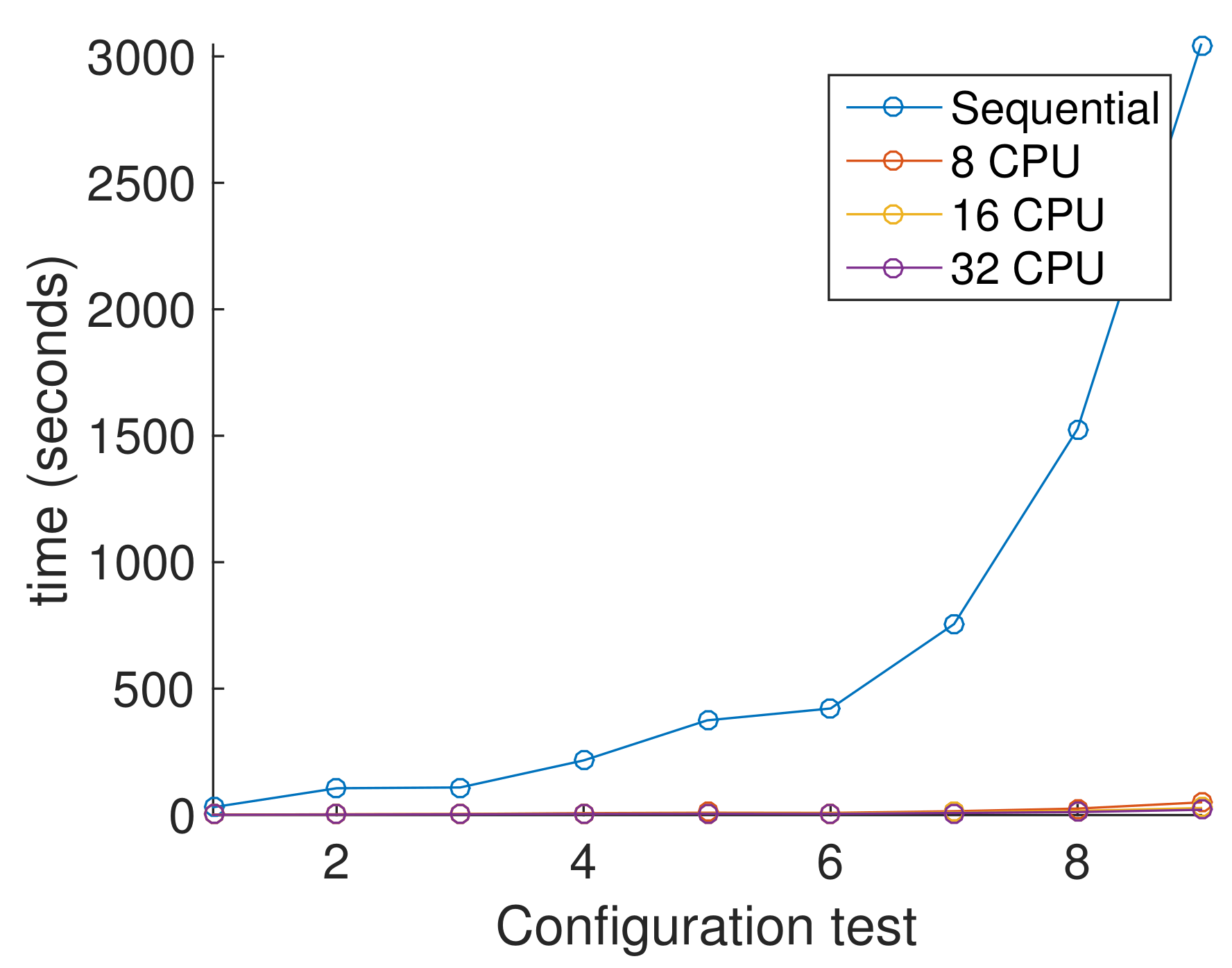
| Islands | Size Island | Knots | Sequential Version Time | Parallel Version | |||||
|---|---|---|---|---|---|---|---|---|---|
| 8 CPUs | 16 CPUs | 32 CPUs | |||||||
| Time | Speed-Up | Time | Speed-Up | Time | Speed-Up | ||||
| 10 | 60 | 50 | 31.14 s | 1.55 s | 20.04 | 1.22 s | 25.59 | 1.10 s | 28.19 |
| 10 | 60 | 100 | 106.15 s | 3.20 s | 33.19 | 2.67 s | 39.72 | 2.01 s | 52.82 |
| 10 | 200 | 50 | 109.21 s | 4.40 s | 24.83 | 3.36 s | 32.50 | 2.82 s | 38.79 |
| 20 | 200 | 50 | 216.14 s | 7.67 s | 28.18 | 5.67 s | 38.15 | 4.47 s | 48.33 |
| 10 | 200 | 100 | 374.60 s | 9.33 s | 40.14 | 6.97 s | 53.75 | 5.14 s | 72.94 |
| 10 | 60 | 200 | 421.54 s | 8.71 s | 48.37 | 7.00 s | 60.24 | 4.84 s | 87.07 |
| 20 | 200 | 100 | 755.32 s | 15.27 s | 49.47 | 10.76 s | 70.21 | 8.33 s | 90.62 |
| 10 | 200 | 200 | 1526.72 s | 25.78 s | 59.21 | 16.57 s | 92.16 | 12.01 s | 127.17 |
| 20 | 200 | 200 | 3046.42 s | 50.27 s | 60.60 | 27.92 s | 109.10 | 20.97 s | 145.30 |
© 2019 by the authors. Licensee MDPI, Basel, Switzerland. This article is an open access article distributed under the terms and conditions of the Creative Commons Attribution (CC BY) license (http://creativecommons.org/licenses/by/4.0/).
Share and Cite
Lara-Ramirez, J.E.; Garcia-Capulin, C.H.; Estudillo-Ayala, M.d.J.; Avina-Cervantes, J.G.; Sanchez-Yanez, R.E.; Rostro-Gonzalez, H. Parallel Hierarchical Genetic Algorithm for Scattered Data Fitting through B-Splines. Appl. Sci. 2019, 9, 2336. https://doi.org/10.3390/app9112336
Lara-Ramirez JE, Garcia-Capulin CH, Estudillo-Ayala MdJ, Avina-Cervantes JG, Sanchez-Yanez RE, Rostro-Gonzalez H. Parallel Hierarchical Genetic Algorithm for Scattered Data Fitting through B-Splines. Applied Sciences. 2019; 9(11):2336. https://doi.org/10.3390/app9112336
Chicago/Turabian StyleLara-Ramirez, Jose Edgar, Carlos Hugo Garcia-Capulin, Maria de Jesus Estudillo-Ayala, Juan Gabriel Avina-Cervantes, Raul Enrique Sanchez-Yanez, and Horacio Rostro-Gonzalez. 2019. "Parallel Hierarchical Genetic Algorithm for Scattered Data Fitting through B-Splines" Applied Sciences 9, no. 11: 2336. https://doi.org/10.3390/app9112336
APA StyleLara-Ramirez, J. E., Garcia-Capulin, C. H., Estudillo-Ayala, M. d. J., Avina-Cervantes, J. G., Sanchez-Yanez, R. E., & Rostro-Gonzalez, H. (2019). Parallel Hierarchical Genetic Algorithm for Scattered Data Fitting through B-Splines. Applied Sciences, 9(11), 2336. https://doi.org/10.3390/app9112336