Abstract
Neural network shows great potential in modulation classification because of its excellent accuracy and achievability but overfitting and memorizing data noise often happen in previous researches on automatic digital modulation classifier. To solve this problem, we utilize two neural networks, namely MentorNet and StudentNet, to construct an automatic modulation classifier, which possesses great performance on the test set with −18–20 dB signal-to-noise ratio (SNR). The MentorNet supervises the training of StudentNet according to curriculum learning, and deals with the overfitting problem in StudentNet. The proposed classifier is verified in several test sets containing additive white Gaussian noise (AWGN), Rayleigh fading, carrier frequency offset and phase offset. Experimental results reveal that the overall accuracy of this classifier for common eleven modulation types was up to 99.3% while the inter-class accuracy could be up to 100%, which was much higher than many other classifiers. Besides, in the presence of interferences, the overall accuracy of this novel classifier still could reach 90% at 10 dB SNR indicting its excellent robustness, which makes it suitable for applications like military electronic warfare.
1. Introduction
An automatic modulation classification task aims at detecting the modulation type of a received signal and recovering the signal by demodulation. Currently, it has been widely used in military electronic warfare, surveillance and threat analysis [1,2]. The likelihood-based (LB) method [3] and feature-based (FB) method [4] are two conventional methods for automatic modulation classification. LB method mainly includes the average likelihood ratio test (ALRT) method [5] and the generalized likelihood ratio test (GLRT) [6]. Although the LB method obtains high accuracy, it requires more calculating time to fulfill parameter estimation, which greatly limits its application [7]. FB methods usually work in two steps: Feature extraction and classification. In previous papers based on FB methods, many signal features, such as spectrum [8], high-order cumulant [9] and wavelet coefficients [10], are used to classify the modulation types. With the emergence and development of machine learning (ML), many researches employ ML to implement classification in FB method. For examples, Aslam et al. [11] reported a modulation classifier based on genetic programming and K-nearest neighbor (GP-KNN), but this classifier only worked well for PSK. Han et al. [12] employed the support vector machine (SVM) to classify the phase shift keying (PSK) and quadrature amplitude modulation (QAM) and obtained a good classification accuracy under the known channel. Although the FB method shows great advantages in automatic digital modulation classification, there are still two challenges: Artificial feature extraction and noise covering. The performance of FB methods severely depends on the quality and quantity of extracted features, but the artificial feature extraction is complex and difficult for various modulated wireless signals. Moreover, when the signal-noise ratio (SNR) of the modulated signal is very low, the performance of classifier is unsatisfied due to the limited quantity of features extracted.
The neural network [13] is a fascinating classification method with a series of state-of-the-art achievements automatic modulation classification [14,15]. For instance, O’Shea et al. [16] trained a deep neural network (DNN) using a baseband IQ waveform to identify modulation. They reported that it was feasible to use DNN for automatic modulation classification and had a better accuracy with low SNR. Ramjee et al. [17] verified the classification performance of long short-term memory (LSTM), convolutional long short-term memory deep neural network (CLDNN) and deep residual network (ResNet) structures. Experimental results showed that the three methods could achieve good classification results on the dataset RadioML2016.10b [16]. The paper also verified the impact of training data with different SNRs, and minimized the training data to reduce training time. However, a neural network is very easy to overfit and memorize data noise when using it in modulation classification [18]. Noises will be introduced into the signal when it goes through channels, inducing a sharp decrease in SNR. If this low SNR data is used to train the neural network, local optimum could appear and cause significant decline in the performance of classifier.
To solve the overfitting of neural network, we propose a novel automatic digital modulation classifier with two neural networks, namely the StudentNet and MentorNet. The StudentNet is used to classify the signal, and the MentorNet is employed to supervise the training of StudentNet according to curriculum learning. Experimental results show that our classifier can accurately identify 11 common digital modulated signals, including 2-ary amplitude shift keying (2ASK), 2-ary Frequency Shift Keying (2FSK), 2PSK, 4ASK, 4FSK, 4PSK, 8ASK, 8FSK, 8PSK, 16QAM and 64QAM. The overall classification accuracy can be up to 99.3%, which is much higher than other classifiers.
The structure of this paper is organized as follows. Section 2 shows the signal model and relative theories. Section 3 presents the performance improvement in modulation classification by curriculum learning. Section 4 reports the experimental results and discussion, and concludes this paper in Section 5.
2. Signal Model and Relative Theories
2.1. Signal Models
The received modulated signal can be expressed as:
where and are the in-phase and quadrature components of IQ modulation, respectively, is the carrier frequency, is the offset of carrier frequency and is the phase offset. in ASK and FSK, and is a variable in FSK. For PSK, the amplitude of modulated signal is fixed but the phase is variable. Therefore, both and are varied while is fixed in PSK. QAM is a hybridization of ASK and PSK, whose amplitude and phase are variables. These features provide possibility for us to classify the modulation type, so that the original signal can be recovered accurately. However, the emerged noise in signal transmission often leads to signal distortion, which imposes a big obstacle in the recovery of the original signal.
Among various noises, additive white Gaussian noise (AWGN) and Rayleigh fading are two most common noises. Therefore, we built models to test the performance of our method in the two above-mentioned noisy environments. Firstly, since AWGN cannot cause the amplitude attenuation and phase offset on signal, the received signal can be expressed as:
where is the additive white noise obeying the zero-mean Gaussian distribution. This model is an effective model to depict the propagation of wired signal, satellite signal and deep space radio frequency communication signal.
Rayleigh fading describes the amplitude attenuation and Doppler shift induced by reflection, refraction, scattering and relative motion between the receiver and the transmitter in the propagation of wireless signal. Once a signal passes through a wireless channel, its amplitude becomes random and its envelope obeys the Rayleigh distribution. According to the central limit theorem, the amplitude of received signal approaches to the zero-mean Gaussian distribution. Since there is no line of sight in Rayleigh channel, the received signal is composed of multi signals suffering reflection, refraction or scattering. Hence, the received signal can be described as:
where means the number of paths, is the path gain of the -th path and is the path gain of the -th delay.
2.2. Deep Residual Network
For the neural network, its classification accuracy depends on the depth of network. With the increase of depth, the classification accuracy firstly improves and then reduces. Researches show that the reduction of classification accuracy is caused by the disappearance of variation in network weight gradient. Aiming at solving this problem, we employ a deep residual network (ResNet), which contains multiple residual blocks as shown in Figure 1a. The residual block mainly includes three convolution layers (Conv layer 1, Conv layer 2 and Conv layer 3) and a summator. There are two routes between these layers and summator: Sequential connection and shortcut connection. Firstly, the sequential connection conducts three consecutive convolutions on x to get F(x), which is used as an input for the summator. Then, the other input of the summator, x, is obtained by shortcut connection. Finally, the output of whole residual block can be expressed as H(x) = F(x) + x. As F(x) = 0 indicates the gradient disappearance of network weight, H(x) = x is an identity mapping that removes the three convolution layers and decreases the depth while the classification accuracy is ensured.
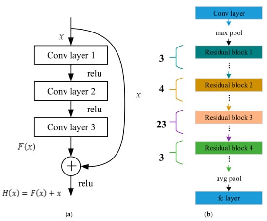
Figure 1.
The architecture of the (a) residual block and (b) ResNet.
The complete architecture of ResNet used in this paper is shown in Figure 1b. It contains a convolution layer, a full connection layer and 33 residual blocks. Every residual block contains three convolution layers. Therefore, the utilized ResNet is a 101-layer DNN. The detailed parameters of ResNet are the same as the 101 layers ResNet parameters [19]. We only modified the input size and output size of the network.
2.3. Curriculum Learning
As known, overfitting occurs easily in the application of a neural network, and curriculum learning provides the possibility to solve this problem. Curriculum learning is inspired by the learning principles behind the cognitive processes of human and animal, which usually begin with learning the easy contents and then gradually consider the more complex parts. According to this learning principle, curriculum learning can assign priority to samples of the training set, such as D = {(x1,y1),⋯(xi,yi),⋯(xn,yn)}, by associating the learning model parameter w and the weight of sample in training set v as follows [20]:
where xi is the ith training sample, yi is the corresponding label, is the discriminative function of a neural network called StudentNet, is the loss function of StudentNet, represents a curriculum and is a variable parameter to tune the learning pace. Although the alternating minimization algorithm is usually employed to minimize Equation (4), it is too complex and requires too much calculation resources. Herein, we employ the scholastic gradient partial descent (SPADE) algorithm [21] based on another neural network named MentorNet to minimize the association of the parameter w of StudentNet and the weights v of random mini-batch samples, so that the bad local minima can be avoided and the better generalization results can be gained.
3. Curriculum Learning Based Modulation Classification
3.1. Architecture of Automatic Digital Modulation Classifier
The diagram of our automatic digital modulation classifier is shown in Figure 2. The input of this classifier is an intermediate frequency signal-containing carrier, which is different from the baseband signal used in previous studies [22,23,24]. Then, the input signal is sampled and normalized to obtain a one-dimensional sequence. Next, the one-dimensional sequence is sliced into multiple short sequences, and a grayscale image is gained by arranging these multiple short sequences row by row. Finally, this grayscale image is considered as the input of StudentNet. In practical applications, the StudentNet needs to be trained under the supervision of MentorNet. Later, we would interpret the training of StudentNet in details.
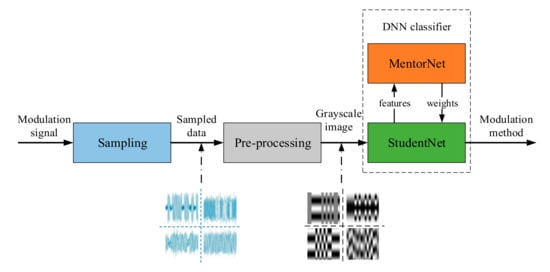
Figure 2.
The diagram of the automatic digital modulation classifier.
3.2. Implementation of MentorNet
The structure of MentorNet is shown in Figure 3. The MentorNet including 10 LSTM (long short-term memory) units can receive new data input and remember the last output. While the input loss value and the difference between loss and the moving average [25] have a time correlation due to the increase of training iteration times, so that the LSTM can predict the weight of samples better. In addition, an embedding layer (size = 5) is employed to receive the integer epoch percentage as its input. Meantime, two fully connected layers fc1 and fc2 contain 20 hidden nodes and one node, separately. The fully connected layer fc2 uses sigmoid as the activation function, ensuring that its output is between 0 and 1. The output layer is a probability sampling layer and its application is to dropout samples with a specific probability. The input of MentorNet is some sample features including aforementioned loss, loss difference to the moving average, and training epoch percentage. The output of MentorNet is weighted corresponding to these features. The loss is calculated by the difference between the actual and predicted modulation types of samples in training set. The moving average is the value of the -th largest loss of features. The training epoch percentage ranging from 0–99 shows the training progress of StudentNet. Zero represents the first training epoch, while 99 symbolizes the last training epoch.
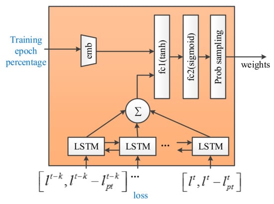
Figure 3.
MentorNet architecture.
The MentorNet is used to supervise the training of StudentNet, so the training of MentorNet should be measured before the StudentNet training. However, in order to obtain the loss, the StudentNet needs to be pre-trained to get the predicted modulation types of samples in training set. In terms of pre-train procession of StudentNet, 18 epoch percentages are trained by using noisy samples, and then we use this trained network to evaluate a noisy test set and get the losses. The average losses under different SNRs are presented in Figure 4. It can be found that when the SNR is larger than 0 dB, the loss varies in a small range, and these samples can be considered as the easy learning samples. Therefore, weights of these samples should be marked as . Once the SNR of samples is less than 0 dB, the loss shows a continuous increase indicating these samples are difficult to learn. Then these samples’ weights could be marked as . These losses and weights obtained by StudentNet are used to train the MentorNet. After training MentorNet, MentorNet has learned this curriculum corresponding to the features mentioned above.
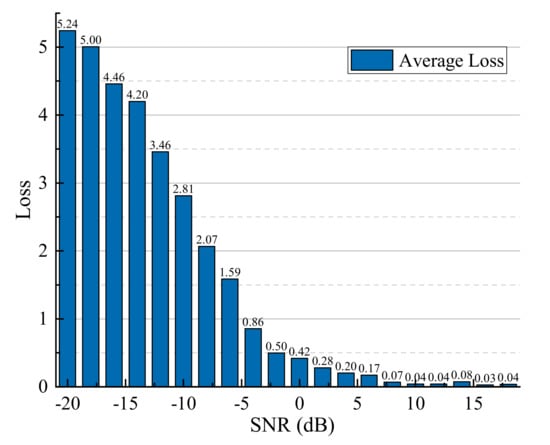
Figure 4.
Average loss of actual and predictive modulation type at different signal-to-noise ratios (SNRs).
Figure 5 illustrates the performance of trained MentorNet. Figure 5a,b represents the schematic diagram of MentorNet assigning weights to samples when training is completed by 20% and 90%. In the Figure 5, epoch percentage represents the percentage of the current training progress, and the z axis represents the weights computed by trained MentorNet, The y axis and the x axis are the sample loss and the difference between sample loss and moving average. For samples with larger loss, the corresponding weight should be smaller, and the rapid decline in different locations means that the courses in these two phases are different. The diff to loss mv can be used to capture the prediction variance [25]. It can be seen that the MentorNet tends to assign high weights to samples with low loss and it can be updated in real time, which provides a great generalization capability for the StudentNet.
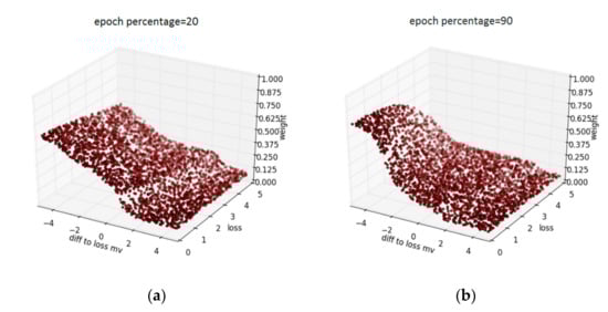
Figure 5.
The data-driven curriculum learned by MentorNet: (a) Epoch percentage = 20 and (b) epoch percentage = 90.
3.3. Implementation of the StudentNet
In our design, the StudentNet should be trained twice. The first training is the pre-training process. Firstly, the pre-training was carried out without the supervision of MentorNet to obtain features of sample in training set. Subsequently, the obtained features were transferred to MentorNet for the extraction of curriculum. Herein, we focus on training the StudentNet under the supervision of MentorNet and testing the performance of the proposed classifier.
The diagram of the second training under the supervision of MentorNet is shown in Figure 6a. Obviously, the StudentNet training can be divided into two steps. The first step is called forward propagation, in which StudentNet obtains the predicted label of training samples by convolution operations and pooling, and then computes the loss between the actual label and predicted label. According to the value of computed losses, the MentorNet assigns corresponding weight to loss. In the second step, named back propagation, the weighted loss is passed back to the upper layer and each layer needs to manipulate own its parameters according to the received loss. After training the StudentNet, the parameters of each layer are saved in a memory.
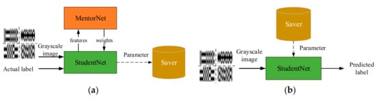
Figure 6.
The diagrams of (a) training StudentNet under the supervision of MentorNet training and (b) testing the performance.
During verifying the performance of our classifier, the parameters are loaded into the StudentNet from memory. Afterwards, the samples in test set are transferred into classifier and processed into grayscale images before coming into the StudentNet. Finally, the predicted labels are obtained by forward propagation. The diagram of performance testing is shown in Figure 6b. Unlike the training of StudentNet, the testing process does not require the involvement of MentorNet and back propagation.
4. Results and Discussion
In this section, a series of measurements are implemented to verify the classification accuracy of the automatic digital modulation classifier. In our experiment, various modulated signals were tested, including 2ASK, 4ASK, 8ASK, 2FSK, 4FSK, 8FSK, 2PSK, 4PSK, 8PSK, 16QAM and 64QAM. The relative parameters are shown in Table 1. We generated a training set and test set by using Matlab2018a. Every training set included 110,000 samples, while each validation set and test set included 11,000 samples. All these samples possessed the same length of 1024 and various SNRs obeying uniform distribution. The training, validation and test sets were used to implement the training, evaluation and exam of classifier, respectively. In addition, the classifier with only StudentNet was named as the Baseline classifier, and the one containing both StudentNet and MentorNet was called the MentorNet classifier.

Table 1.
Modulation parameter.
4.1. The Accuracy of MentorNet Classifier
4.1.1. Overall Accuracy of MentorNet Classifier Under Different SNRs
Before investigating the performance of MentorNet classifier, the Baseline classifier was established and trained by four training set with different SNR ranges. Herein, samples in the training set and test set were the signals passing through additive white Gaussian channel without phase drift and frequency drift Therefore, SNR was the ratio between the amplitudes of Gaussian noise and signal. Then the performance of trained Baseline classifiers was measured on one test set with SNRs ranging from to 18 dB and the results are shown in Figure 7a. It is obvious that when the SNR of the training set was relatively high (such as 10–18 dB, Black line in Figure 7a), the Baseline classifier possessed higher classification accuracy, whereas an unsatisfactory performance occurred on the samples with low SNR in the test set. Unfortunately, once the SNR range of the training set broadened to −20–18 dB (Purple line in Figure 7a), the performance of the Baseline classifier showed an improvement on samples with low SNR in the test set but deterioration on samples with high SNR in the test set. We suppose this phenomenon should be induced by the overfitting of StudentNet in the Baseline classifier. To overcome this problem, the MentorNet classifier was proposed and tested. The MentorNet classifier was trained by only one training set with −20–18 dB SNR and its performance was verified on the same test set with the Baseline classifier. The green and magenta curves in Figure 7a revealed that for the training set with −20–18 dB SNR, the MentorNet classifier could overcome the overfitting, and results in a 1.7% improvement in classification accuracy.
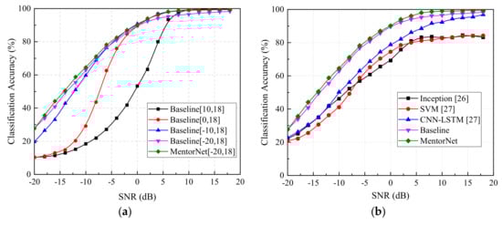
Figure 7.
The performance of various classifiers under different SNRs: (a) Curves about the classification accuracy versus the SNR range of the training set, and (b) classification accuracy of different methods with −20–18 dB SNR.
Besides, we also compared the accuracy of the MentorNet classifier with several existing modulation classifiers, including the classifiers based on the Inception [26], the fusion model of convolutional neural network and long short-term memory (CNN-LSTM) [27], and SVM [27]. The five classifiers were trained and tested with the same training set and test set, and then the classification accuracy are shown in Figure 7b. Comparison results indicated that both the accuracy of the MentorNet classifier and Baseline classifier was higher than others, which verifies that ResNet could improve the classification accuracy significantly. Due to the existence of overfitting in the Baseline classifier, its performance was worse than the MentorNet classifier. Therefore, we can conclude that the MentorNet classifier proposed by us could achieve the higher classification accuracy.
4.1.2. Intra-Class and Inter-Class Accuracy of the MentorNet Classifier Under Different SNRs
In addition to the overall accuracy, the intra-class and inter-class accuracy of the classifier is also worthy to mention. The common modulation signals can be divided into four classes including ASK, FSK, PSK and QAM according to the modulation method. According to the modulation order, these four classes also can be divided into eleven types, including 2ASK, 4ASK, 8ASK, 2FSK, 4FSK, 8FSK, 2PSK, 4PSK, 8PSK, 16QAM and 64QAM. The intra-class accuracy of MentorNet classifier for each modulation class at different SNR is reported in Figure 8, which denotes that all classification accuracy increased with SNR until approaches closed to 100%. In details, when SNR was larger than –10 dB, the classification accuracy of 2ASK was largest in ASK and saturated at 10 dB. Meantime, the classification accuracy of 2PSK was also the largest in PSK and saturated at −10 dB. Besides, the modulation order had few impacts on the classification accuracy of FSK as SNR was lower than 0 dB. However, the intra-class accuracy of QAM was almost unaffected by the modulation order. These results suggest that the modulation order has a different influence on the intra-class accuracy of different classes.
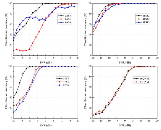
Figure 8.
Curves about intra-class classification accuracy versus SNR.
The inter-class accuracy of MentorNet classifier was obtained by its confusion matrix as shown in Figure 9. The confusion matrix illustrates the prediction error of the classifier, where the horizontal and vertical axes represent the actual and predicted modulation types. The inter-class accuracy was calculated by ignoring the modulation order and adding the probability of achieving the correct modulation class. From Figure 9, we can conclude that it was difficult to identify both the modulation order and the modulation class accurately at low SNR (such as −20 dB) due to the large noise interference, which is consistent with Figure 7 and Figure 8. It is well-known that the wrong modulation order cannot pose a fatal threat to the demodulated signal so that the demodulated signal showed a large deviation with the original signal. The correct modulation class was the most urgent need for us. Hence, we presented the inter-class accuracy of MentorNet classifier in Figure 10. As shown in Figure 10, the MentorNet classifier could effectively distinguish modulation classes such as ASK, FSK and PSK even if SNR was very low (such as −20 dB). However, the inter-class accuracy of QAM was relatively low as SNR was lower than –10 dB, because QAM was easy to be recognized as PSK according to Figure 9. However, the original signal of QAM can be recovered by conventional demodulation in the case of misjudgment. Therefore, the performance of the MentorNet classifier could satisfy the accuracy requirements for modulation recognition in most applications.
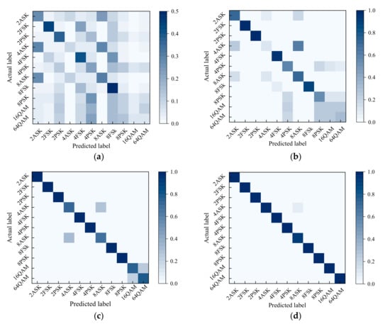
Figure 9.
Confusion matrix with different SNRs: (a) SNR = −20 dB; (b) SNR = −10 dB; (c) SNR = 0 dB and (d) SNR = 10 dB.
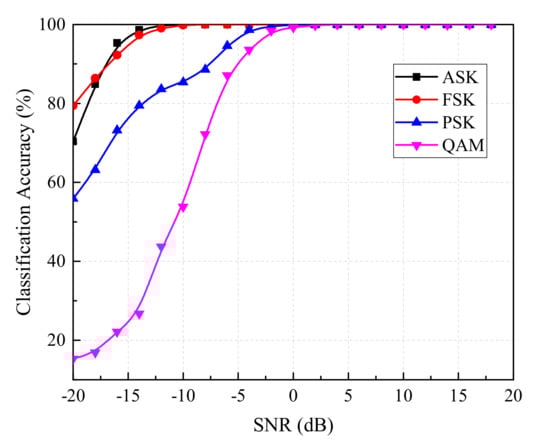
Figure 10.
Curves about inter-class classification accuracy versus SNR.
4.2. The Robustness of the MentorNet Classifier
4.2.1. The Impact of Rayleigh Fading
As known, AWGN and Rayleigh fading are two common noise sources. The samples with AWGN have been tested above. Hence, this subsection will investigate the impact of Rayleigh fading on the accuracy of the MentorNet classifier. In the experiment, the modulation parameters and the number of samples in the test set were the same as above. Besides, we assumed that the received signal was a combination of two signals coming from two reflection paths. The gains of these two paths were 0 dB and −10 dB, respectively, while the delay between them was s. In the meantime, the maximum Doppler frequency shift (fd), induced by the relative motion between the receiver and the transmitter in the propagation of two signals, was supposed as 0 Hz, 1 kHz, 5 kHz and 10 kHz.
The experimental results are shown in Figure 11. It is worth mentioning that the black and red curves both represent the classification accuracy of test samples with a 0 Hz Doppler shift, but a multipath fading existed in the test samples of the red curves, leading to the relatively low classification accuracy. However, the red curve could also reach 20% at −20 dB SNR and 99% at 10 dB SNR, which was close to the black curve. When the different Doppler shifts existed, the classification accuracy at very low SNR (such as −20 dB) was very similar until the SNR was up to −5 dB. With the further increase of SNR, the difference of classification accuracy increased and a larger Doppler shift corresponded to a lower classification accuracy classifier. When the SNR was 10 dB the classification accuracy of test samples containing Rayleigh fading ranged from 85% to 98%, which is enough for the application in military electronic warfare equipment. These results indicate the MentorNet classifier possesses a great robustness to endure the Rayleigh fading.
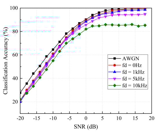
Figure 11.
Classification accuracy of the MentorNet classifier under the interference of Rayleigh fading.
4.2.2. The Impact of Carrier Frequency Offset and Phase Offset
As shown in Equation (1), the carrier frequency offset and phase offset induced by the drift of the clock could also increase the difficulty of modulation classification. In this subsection, we would explore the impact of carrier frequency offset and phase offset on the classification accuracy of the MentorNet classifier. Firstly, the ratio of carrier frequency deviation to sampling frequency was set within to investigate the anti-interference ability of the MentorNet classifier to carrier frequency offset. For a fair comparison, the Inception classifier, Baseline classifier and MentorNet classifier were trained by a training set with −20–18 dB SNR, and then they were tested in a test set with an SNR of 10 dB. The experimental results are reported in Figure 12a. We could find the accuracy of all classifier decreased monotonously with , but the reduction of Inception classifier was the smallest (around 5%), due to its simple network structure [28] Meanwhile the reductions of the Baseline classifier and MentorNet classifier were around 13% and 12% separately. Although the accuracy of the Baseline classifier and MentorNet classifier was significantly disturbed by the carrier frequency offset, their accuracy was still 14% and 18% higher than the Inception classifier, respectively. Hence, it was obtained that in the presence of frequency offset, the performance of the MentorNet classifier was still the best, so that has actual importance in the field of communication.
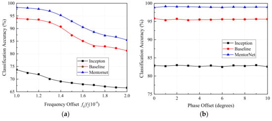
Figure 12.
Classification accuracy with (a) different carrier frequency offsets and (b) different phase offsets.
Then, the impact of the phase offset on the accuracy of the classifier was studied and discussed. The experimental parameters are the same as above, except the carrier frequency offset and phase offset. The phase offset was set within 0–10, while the carrier frequency offset was set to 0 Hz. The results are shown in Figure 12b. It is obvious that the phase offset had little effect on the accuracy of classifier, which suggests the strong robustness to phase offset. Moreover, the accuracy of the MentorNet classifier could maintain at 99% regardless of the phase offset, while the Inception classifier and Baseline classifier could only achieve a classification accuracy of 96% and 83%, respectively. This phenomenon reveals that among these three classifiers, the designed MentorNet classifier obtained a better performance.
4.3. Classification Accuracy on a Generic Dataset
An additional experiment was conducted to evaluate the classification performance on analog modulation signals, and a GUN radio generated dataset (RML2016b) was used [16]. In the test, the dataset was divided into a training set, validation set and test set. We used the training set to train StudentNet, and used the validation set to evaluate the performance of the current classifier and select the best classifier for testing. For the MentorNet classifier, the trained MentorNet was used to supervise the training of StudentNet. For the Baseline classifier, the StudentNet was trained without MentorNet. As shown in Figure 13, the comparison of classification accuracy was made among MentorNet classifier and some classical methods such as the Baseline, ResNet and CLDNN [29] classifiers. When the SNR was greater than 0 dB, our proposed MentorNet classifier could achieve the overall classification accuracy up to 85.5%, which was better than the Baseline (82.2%), CLDNN (83.1%) and ResNet (80.5%). The comparison results indicate that the proposed MentorNet classifier could also deal with the analog modulation signals with better versatility and classification accuracy.
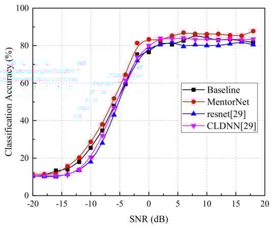
Figure 13.
Classification accuracy of various classifiers on dataset RML2016b.
5. Conclusions
In this paper, we reported a novel automatic digital modulation classifier called the MentorNet classifier, which consists of two neural networks: StudentNet and MentorNet. The MentorNet supervises the training of StudentNet to overcome the overfitting in the classification process. In order to verify the performance of this classifier, several comparative tests with other classifiers were conducted in the presence of AWGN, Rayleigh fading, carrier frequency offset and phase offset. Experimental results showed the accuracy of the MentorNet classifier and Baseline classifier was much higher than the Inception classifier and classifier based on SVM, which suggests the deep residual network is suitable for digital modulation classification. Meantime, the accuracy of the MentorNet classifier at high SNR was higher than that of the Baseline classifier, indicating the curriculum learning can solve the overfitting of the neural network. In the interference of Rayleigh fading, the MentorNet classifier still owned the highest accuracy, which ranged from 80%–90% at 10 dB SNR as the Doppler frequency shift was within 0–10 kHz, which suggests the outstanding robustness of MentorNet classifier. When the carrier frequency offset and phase offset were taken into account, the accuracy of the MentorNet classifier presented quite different tendencies. When only the carrier frequency offset was considered, the accuracy of the MentorNet classifier showed a smooth reduction from 98% to 85% with ranging within , while it maintained at 99% in the presence of a 0–10 phase offset. Moreover, the proposed classifier could also achieve favorable classification performance for analog baseband signals, indicating the transplantation feasibility of the proposed classifier. Although the proposed MentorNet classifier had outstanding performance, when SNR was −20 dB the classification accuracy remains to be improved.
Author Contributions
M.Z., H.W. and Z.Y. conceived and designed the experiments; H.Q. performed the experiments; Y.L., Z.Y. and W.Z. analyzed the data; H.W. and M.Z. contributed analysis tools; and M.Z. and Z.Y. wrote the paper.
Funding
This research was funded by the China Postdoctoral Science Foundation (2018M633471), the National Natural Science Foundation of Shaanxi Province under Grant (2019JQ-270), the AeroSpace T.T. and C. Innovation Program and the China Scholarship Council (201806965054).
Conflicts of Interest
The authors declare no conflict of interest.
References
- Azzouz, E.; Nandi, A.K. Automatic Modulation Recognition of Communication Signals; Springer Science & Business Media: Berlin, Germany, 2013. [Google Scholar]
- Nandi, A.K.; Azzouz, E.E. Algorithms for automatic modulation recognition of communication signals. IEEE Trans. Commun. 1998, 46, 431–436. [Google Scholar] [CrossRef]
- Zhu, Z.; Nandi, A.K. Automatic Modulation Classification: Principles, Algorithms and Applications; John Wiley & Sons: Hoboken, NJ, USA, 2014. [Google Scholar]
- Hazza, A.; Shoaib, M.; Alshebeili, S.A.; Fahad, A. An overview of feature-based methods for digital modulation classification. In Proceedings of the 2013 1st International Conference on Communications, Signal Processing, and Their Applications (ICCSPA), Sharjah, UAE, 12–14 Feburary 2013; pp. 1–6. [Google Scholar]
- Wei, W.; Mendel, J.M. Maximum-likelihood classification for digital amplitude-phase modulations. IEEE Trans. Commun. 2000, 48, 189–193. [Google Scholar] [CrossRef]
- Hameed, F.; Dobre, O.A.; Popescu, D.C. On the likelihood-based approach to modulation classification. IEEE Trans. Wirel. Commun. 2009, 8, 5884–5892. [Google Scholar] [CrossRef]
- Dobre, O.A.; Abdi, A.; Bar-Ness, Y.; Su, W. Survey of automatic modulation classification techniques: Classical approaches and new trends. IET Commun. 2007, 1, 137–156. [Google Scholar] [CrossRef]
- Gardner, W.A. Signal interception: A unifying theoretical framework for feature detection. IEEE Trans. Commun. 1988, 36, 897–906. [Google Scholar] [CrossRef]
- Dandawate, A.V.; Giannakis, G.B. Statistical tests for presence of cyclostationarity. IEEE Trans. Signal Process. 1994, 42, 2355–2369. [Google Scholar] [CrossRef]
- Dan, W.; Xuemai, G.; Qing, G. A new scheme of automatic modulation classification using wavelet and WSVM. In Proceedings of the Second International Conference on Mobile Technology, Applications and Systems (IEE Mobility Conference 2005), Guangzhou, China, 15–17 November 2005. [Google Scholar]
- Aslam, M.W.; Zhu, Z.; Nandi, A.K. Automatic modulation classification using combination of genetic programming and KNN. IEEE Trans. Wirel. Commun. 2012, 11, 2742–2750. [Google Scholar]
- Han, L.; Gao, F.; Li, Z.; Dobre, O.A. Low complexity automatic modulation classification based on order-statistics. IEEE Trans. Wirel. Commun. 2017, 16, 400–411. [Google Scholar] [CrossRef]
- LeCun, Y.; Bengio, Y.; Hinton, G. Deep learning. Nature 2015, 521, 436–444. [Google Scholar] [CrossRef] [PubMed]
- Khan, F.N.; Teow, C.H.; Kiu, S.G.; Tan, M.C.; Zhou, Y.; Al-Arashi, W.H.; Lau, A.P.T.; Lu, C. Automatic modulation format/bit-rate classification and signal-to-noise ratio estimation using asynchronous delay-tap sampling. Comput. Electr. Eng. 2015, 47, 126–133. [Google Scholar] [CrossRef]
- Khan, F.; Lu, C.; Lau, A. Joint modulation format/bit-rate classification and signal-to-noise ratio estimation in multipath fading channels using deep machine learning. Electron. Lett. 2016, 52, 1272–1274. [Google Scholar] [CrossRef]
- O’Shea, T.J.; Corgan, J.; Clancy, T.C. Convolutional radio modulation recognition networks. In International Conference on Engineering Applications of Neural Networks; Springer: Cham, Switzerland, 2016; pp. 213–226. [Google Scholar]
- Ramjee, S.; Ju, S.; Yang, D.; Liu, X.; Gamal, A.E.; Eldar, Y.C. Fast Deep Learning for Automatic Modulation Classification. arXiv 2019, arXiv:1901.05850. [Google Scholar]
- Zhang, C.; Bengio, S.; Hardt, M.; Recht, B.; Vinyals, O. Understanding deep learning requires rethinking generalization. arXiv 2016, arXiv:1611.03530. [Google Scholar]
- He, K.; Zhang, X.; Ren, S.; Sun, J. Deep residual learning for image recognition. In Proceedings of the IEEE Conference on Computer Vision and Pattern Recognition, Las Vegas, NV, USA, 26 June–1 July 2016; pp. 770–778. [Google Scholar]
- Jiang, L.; Meng, D.; Zhao, Q.; Shan, S.; Hauptmann, A.G. Self-Paced Curriculum Learning. In Proceedings of the Twenty-Ninth AAAI Conference on Artificial Intelligence, Austin, TX, USA, 25–30 January 2015; p. 6. [Google Scholar]
- Jiang, L.; Zhou, Z.; Leung, T.; Li, L.-J.; Fei-Fei, L. MentorNet: Learning Data-Driven Curriculum for Very Deep Neural Networks on Corrupted Labels. arXiv 2017, arXiv:1712.05055. [Google Scholar]
- Ali, A.; Yangyu, F. Unsupervised feature learning and automatic modulation classification using deep learning model. Phys. Commun. 2017, 25, 75–84. [Google Scholar] [CrossRef]
- Almohamad, T.A.; Salleh, M.F.M.; Mahmud, M.N.; Sa’d, A.H.Y. Simultaneous Determination of Modulation Types and Signal-to-Noise Ratios Using Feature-Based Approach. IEEE Access 2018, 6, 9262–9271. [Google Scholar] [CrossRef]
- Hussain, A.; Sohail, M.; Alam, S.; Ghauri, S.A.; Qureshi, I. Classification of M-QAM and M-PSK signals using genetic programming (GP). In Neural Computing and Applications; Springer: Basingstoke, UK; pp. 1–9.
- Chang, H.-S.; Learned-Miller, E.; McCallum, A. Active Bias: Training More Accurate Neural Networks by Emphasizing High Variance Samples. In Proceedings of the Thirty-First Annual Conference on Neural Information Processing Systems, Long Beach, CA, USA, 4–9 December 2017; pp. 1002–1012. [Google Scholar]
- Szegedy, C.; Liu, W.; Jia, Y.; Sermanet, P.; Reed, S.; Anguelov, D.; Erhan, D.; Vanhoucke, V.; Rabinovich, A. Going deeper with convolutions. In Proceedings of the IEEE Conference on Computer Vision and Pattern Recognition, Boston, MA, USA, 7–12 June 2015; pp. 1–9. [Google Scholar]
- Zhang, D.; Ding, W.; Zhang, B.; Xie, C.; Li, H.; Liu, C.; Han, J. Automatic Modulation Classification Based on Deep Learning for Unmanned Aerial Vehicles. Sensors 2018, 18, 924. [Google Scholar] [CrossRef] [PubMed]
- Su, D.; Zhang, H.; Chen, H.; Yi, J.; Chen, P.-Y.; Gao, Y. Is robustness the cost of accuracy?—A comprehensive study on the robustness of 18 deep image classification models. In Proceedings of the European Conference on Computer Vision, Munich, Germany, 8–14 September 2018; pp. 644–661. [Google Scholar]
- West, N.E.; O’Shea, T. Deep architectures for modulation recognition. Proceedings of 2017 IEEE International Symposium on Dynamic Spectrum Access Networks (DySPAN), Piscataway, NJ, USA, 6–9 March 2017; pp. 1–6. [Google Scholar]
© 2019 by the authors. Licensee MDPI, Basel, Switzerland. This article is an open access article distributed under the terms and conditions of the Creative Commons Attribution (CC BY) license (http://creativecommons.org/licenses/by/4.0/).