3.1. Worm-Inspired Motion Process
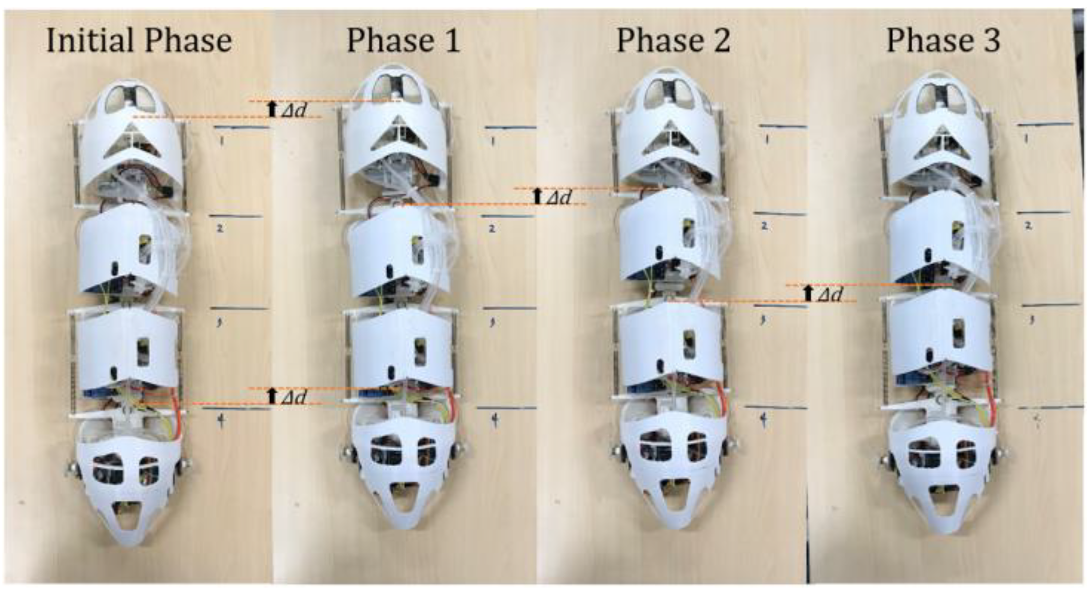
Similar to the worm movement in nature, the motion of this robot is in cycles. During each movement cycle, each segment of the worm-like robot moves forward once one by one to achieve the forward movement of the overall position. In particular, for this robot prototype, its motion cycle is divided into three phases. Assume that the state in the initial phase is as follows: cylinders in Segment 1 and Segment 2 are in the shortened state, the cylinder in the Segment 3 is in the extended state, and each foot is adsorbed on the working surface. Then, the following movements occur during the next motion cycle:
Phase 1: The feet of Segment 1 and Segment 4 are off the work surface and lifted; the remaining feet are still attached to the work surface. Then, the cylinders of Segment 1 extend and the cylinder of Segment 3 shortens; thus, Segment 1 and Segment 4 move forward until the limit stroke of the cylinder. After that, the motor drives the feet of Segment 1 and Segment 4 to be lowered, and a negative pressure is generated in the suction cups, which is then adsorbed on the working surface.
Phase 2: The feet of Segment 2 are off the work surface and lifted; the remaining feet are still attached to the work surface. Then, the cylinders of Segment 1 shorten, and the cylinder of Segment 2 extends; thus, Segment 2 moves forward until the limit stroke of the cylinder. After that, the motor drives the feet of Segment 2 to be lowered, and a negative pressure is generated in the suction cups, which is then adsorbed on the working surface.
Phase 3: The feet of Segment 3 are off the work surface and lifted; the remaining feet are still attached to the work surface. Then, the cylinders of Segment 3 extend, and the cylinder of Segment 2 shortens; thus, Segment 3 moves forward until the limit stroke of the cylinder. After that, the motor drives the feet of Segment 3 to be lowered, and a negative pressure is generated in the suction cups, which is then adsorbed on the working surface.
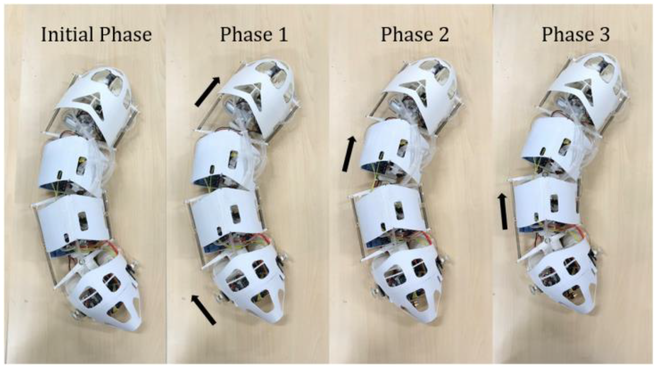
The steering motion of the worm-like robot takes place in Phase 1. When the feet of Segment 1 and Segment 4 are separated from the work surface and lifted, Segment 1 and Segment 4 are deflected to one side, centering on the hinge point by controlling the length of the tendons on the left and right sides. In subsequent movements, the robot will achieve a steering creep movement in one direction. The specific parameter control will be analyzed in
Section 3.2.
The specific work processes of linear crawling and steering crawling are shown in
Figure 5 and
Figure 6, respectively.
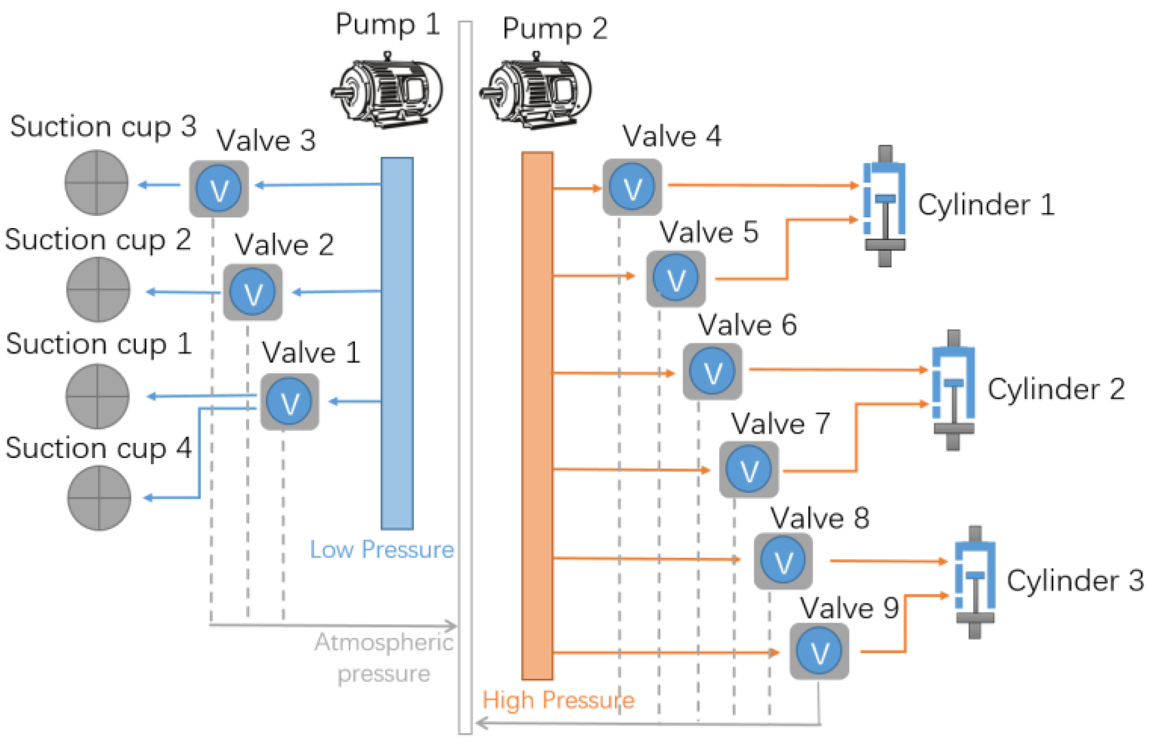
Figure 7 shows the input signal variation of the valve system shown in
Figure 4 during a single motion cycle. It can be seen that in Phase 1, there are two segments in motion at the same time, which is a little different from phases 2 and 3, where there is only one segment in motion, respectively.
3.2. Crawling Process Analysis
The movement of this worm-inspired robot as it crawls in straight lines and turns is briefly described in
Section 3.1 above. The straight crawling motion of the robot is very simple; thus, it will not be discussed here. However, the parameter control during the more complicated steering motion, that is, the specific influences of the tendons’ length on the robot posture and the subsequent motion process, is not analyzed in detail above. So, in this regard, this segment will discuss the above issue in detail.
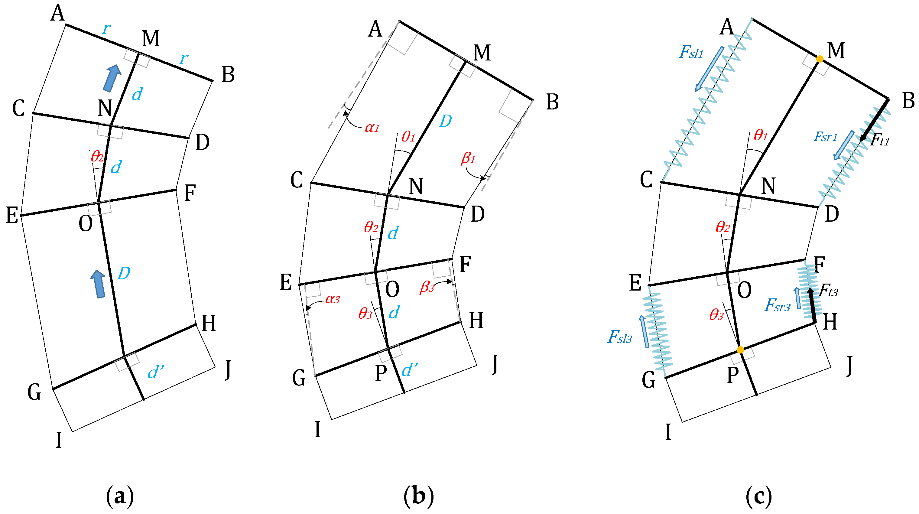
Taking the steering movement to the right as an example, as shown in
Figure 8a,b, we define
,
and
as the deflection angles of Segment 1, Segment 2, and Segment 3 of the robot, respectively.
In Phase 1, segments 1 and 4 move forward, while segments 2 and 3 are consolidated with the ground, so the deflection angle is constant. At the end of Phase 1, and are mainly affected by the lengths and of the left and right tendons, so the values of and can be adjusted by changing the values of and . In this way, the head and tail of this robot are deflected to one side, producing an effect similar to the worm’s steering. Assuming that width (AB) of the worm-like robot is 2r, the length of the cylinder and , and the length of tendon (GI) from pulley to reel in Segment 4 is , the geometric algorithm for the robot posture at the end of Phase 1 is solved below.
The following can be obtained from the geometric relationship:
The above parameters meet:
With the simultaneous use of equations of (10) and (11),
and
that satisfy the condition alone can be found, thereby determining the result of the robot’s geometric posture at the end of the Phase 1. However, through building the prototype, we found in the experiment that due to the slight elastic deformation of the tendon, the actual and the theoretical values have a large deviation. Therefore, we introduced a set of springs, as shown in
Figure 8c, whose original length is
, and elastic coefficient is k, and is connected between B and D, F and H, E and G, C and A, forming a new set of constraint relationships. However, in order to prevent the over-constrained phenomenon caused by the overlapping of the constraint relationship with the original geometric constraint, we put the tendon on the left in a relatively slack state (tension T is 0), thereby canceling one of the original constraints (relationship (10)).
From the perspective of force balance, since Segment 2 and Segment 3 remain stationary in Phase 1, Segment 1 can be regarded as rotating around the N-point hinge. In the figure, assuming that the deflection angle of the left spring (the angle between AC and MN) is
, and the deflection angle of right spring (the angle between BD and the cylinder axis direction of Segment 1 (MN) is
, then the torque generated by the spring force is:
Assuming that the tendon on the right side has a pulling force of
on Segment 1, the torque generated is:
According to the torque balance and simultaneous use of equations of (12) and (13), we can get:
Similarly, segments 3 and 4 can be seen as rotating around the P-point hinge. Assuming that the deflection angle of the left spring (the angle between EG and the cylinder of Segment 3 (OP)) is
, and the deflection angle of the right spring (the angle between FH and OP) is
, then the torque generated by the spring force is:
Assuming that the tendon on the right side has a pulling force of
on Segment 4, the torque generated is:
According to the torque balance and simultaneous use of Equations (17) and (18), we can get:
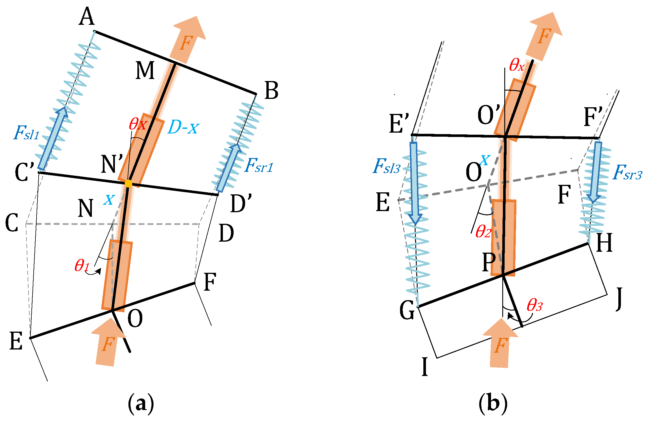
The experiment found that during the movement in Phase 1, due to the large tension in the tendon, it rubs against the pulleys at the corner, and therefore, there is a large resistance. As a result, the actual pulling force of the tendon acting at point B is greater than that at the point H, imposing a greater impact on the actual and . Since the deflection angle of the tendon is circular, the Euler–Eytelwein equation can be used to calculate the resistance, where is the friction coefficient between the tendon and the reel, and is the angle difference of the tendon between point B and point H.
By geometric relationship:
Then, the tension of the tendon to the two points of H and B satisfies:
According to the simultaneous use of Equations (16), (21), and (23), we can get the force constraint:
where
,
,
and
meet:
In summary, according to the simultaneous use of Equations (11) and (24), the values of
and
at the end of Phase 1 can be obtained. Bringing the known related parameters
,
,
,
,
, and
, we calculated the variation of deflection angles
and
with different
values when
is in the initial phase, which is also experimentally measured, and the results are shown in
Figure 9a. We also calculated the variation of deflection angles
and
with different
values when
in the initial phase, which is also experimentally measured, and the results are shown in
Figure 9b.
As is shown in
Figure 9a,b, the theoretical value of
is smaller than
at any condition due to the large frictional resistance along the tendons; such a difference may lower the efficiency of the steering motion. The experiment results are basically in accord with the theory. However, the difference between
and
shown in the experiments seems to be larger than theoretical expectation, which might be caused by the friction on the bearings and the elasticity of the pipelines.
As
is known, and
and
can be solved, we can further solve the length of the left tendon
. As described above, at this time, the left tendon is in a slack state, and the internal tension is 0. In order to satisfy this requirement, the length of the left tendon must not be less than a geometric minimum
:
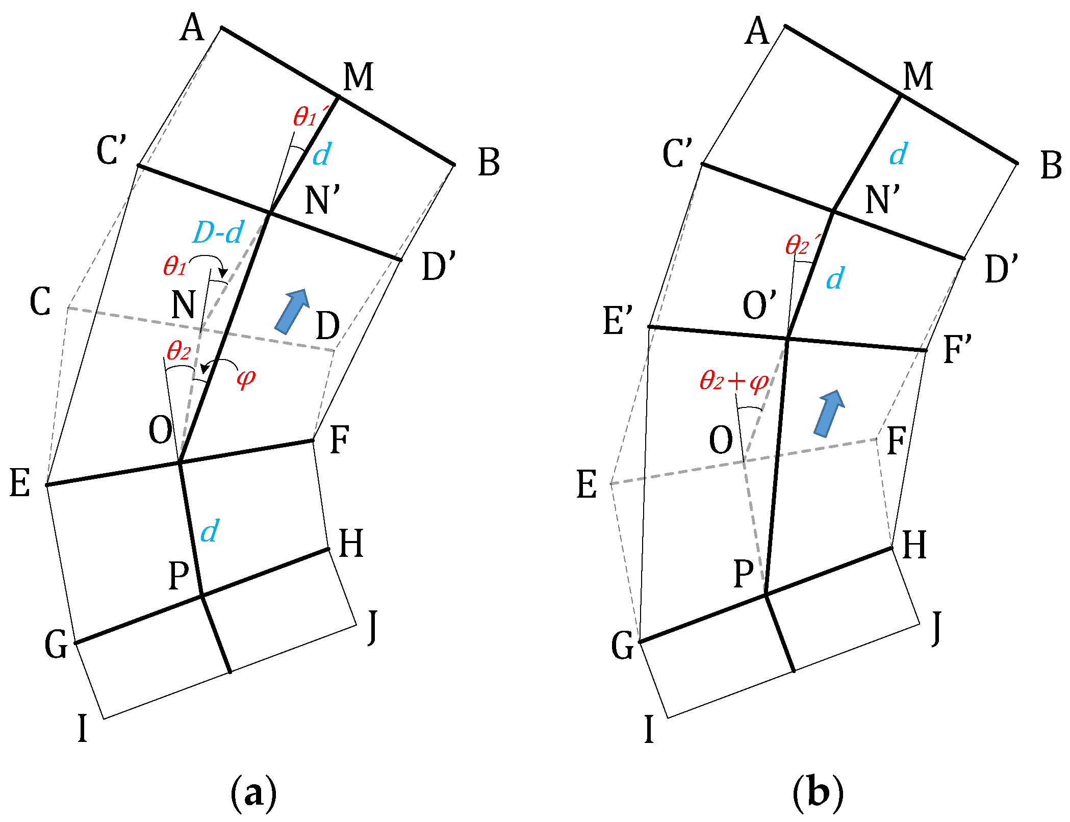
In Phase 2, segments 1, 3, and 4 remain fixed, and as shown in
Figure 10a, point C, D, and N on Segment 2 advance to the positions of the C′, D′, and N′, respectively. At this time, the length of MN′ (the cylinder length of Segment 1) is d, the length of NN′ is D-d, and the deflection angle of Segment 1 becomes
. From the geometric relationship, we can get:
According to the simultaneous use of Equations (29) and (30), the following is obtained:
In Phase 3, segments 1, 2, and 4 remain fixed, and as shown in
Figure 10b, points E, F, and O on Segment 3 advance to the positions of the E′, F′, and O′, respectively. At this time, the length of O′N′ is d, and the deflection angle of Segment 2 becomes
, as shown in
Figure 10b. From the geometric relationship, we can get:
According to simultaneous use of Equations (35) and (34), the value of
at the end of Phase 3 is obtained:
At this point, a motion cycle ends, and the robot returns to the state at the beginning of step 1. Based on the above Equations (11), (24), and (37), the values of
,
, and
after any of the periodic motions can be solved. The relationship between the three values and the number of cycles T is shown in
Figure 11a. It can be seen that regardless of the initial state, after several cycles of the motion,
,
, and
will tend to a fixed value.
In addition, at the end of a motion cycle, the cylinder axis direction of Segment 2 (ON) will have a steering angle
with respect to its original position, and we define
as the steering angle of the robot. After a plurality of cycles, the cumulative value of the angle is defined as the cumulative steering angle ∑
of the robot, which represents the direction change of the overall robot. The relationship between
and ∑
and the number of cycles T is shown in
Figure 11b, from which it can be seen that after the start of the motion, the steering angle tends to a fixed value, and the cumulative steering angle is approximately linear with the number of cycles.
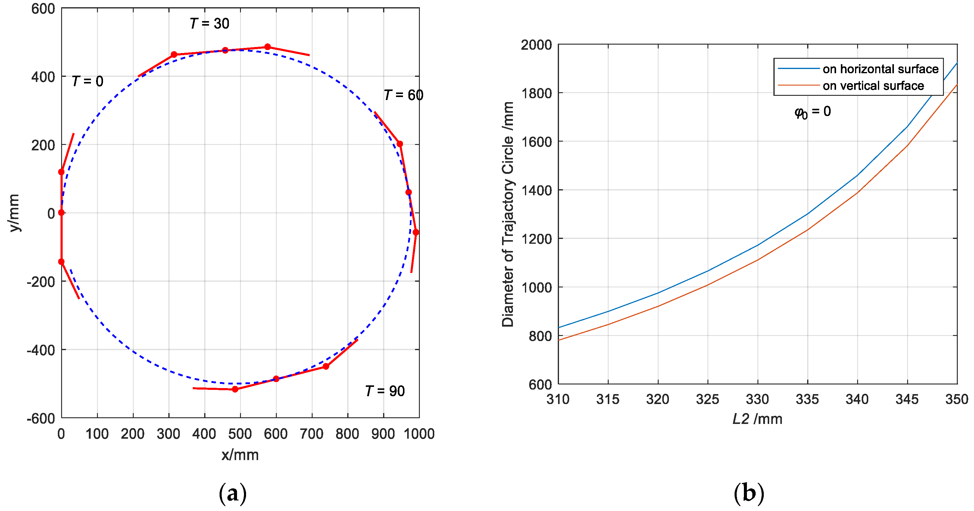
We calculate the trajectory of the robot in 120 motion cycles; the result is shown in
Figure 12a. The figure shows that the motion trajectory of the robot appears to be circular if the length of the tendon remains unchanged. In a particular state, when the length of the tendon (
L2) is 400 mm, the diameter of the trajectory circle is 920 mm.
We conducted an experiment to test the steering ability of the robot. In the experiment, the robot finished a circular route and finally returned to its starting point in 128 motion cycles; the whole process took 22 minutes. The diameter of the circle is 978 mm, which is slightly bigger than the calculation results. Besides the reason of friction, which has been mentioned before, such difference might also be caused by the slippage that happened between the sucker cups and the ground.
With a scalable structure design, the robot can be added to five or more segments in practical application. In these cases, the above calculation results will be slightly different. Take an expanded robot with
n segments in total for example; a single motion cycle described in
Section 3.1 will consist of
n−1 phases (
. During Phase 1, Segment 1 and Segment
n move forward, while the others remain attached to the ground. In this process, we can still control the first and last deflection angle,
and
through adjusting the length of tendons, where the geometric relationship still follows the Equations (11) and (24). In any of the latter phases, only one segment moves forward, and its deflection angle and position can be solved using Equations (35) and (37). Therefore, the position and posture of the robot after a whole cycle can be precisely obtained after the motions in each phase are solved successively.


