Modeling and Analysis of the Influence of an Edge Filter on the Combining Efficiency and Beam Quality of a 10-kW-Class Spectral Beam-Combining System

Abstract
Featured Application
Abstract
1. Introduction
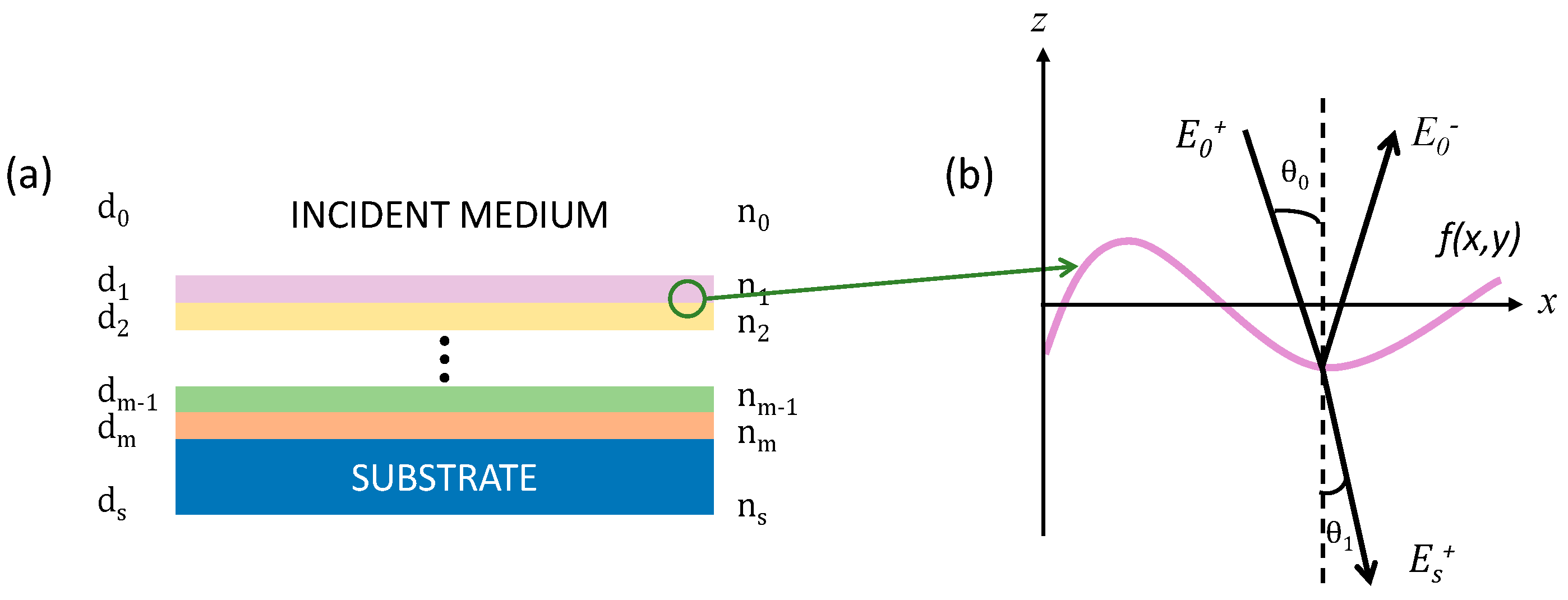
2. Theory
3. Simulation and Experimental Results
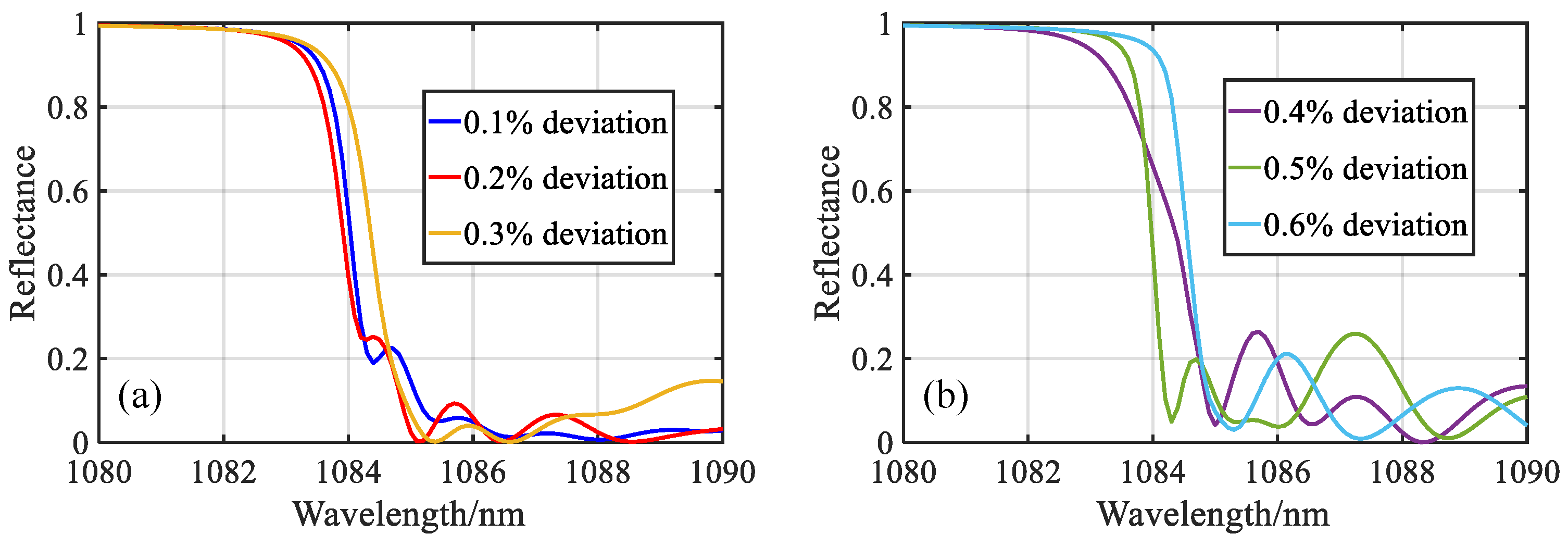
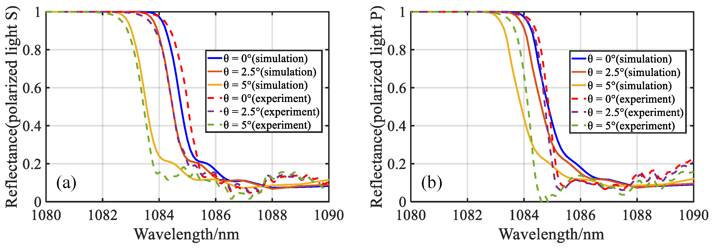
3.1. The Reflectance Curve of the Edge Filter
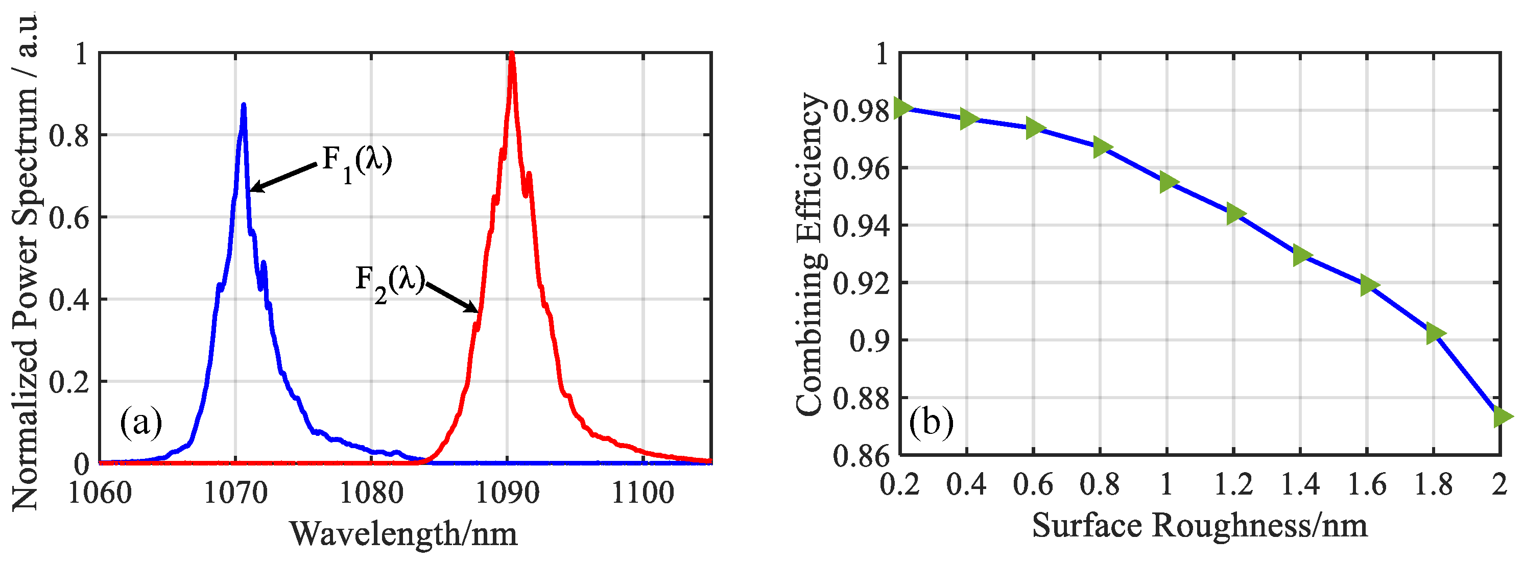
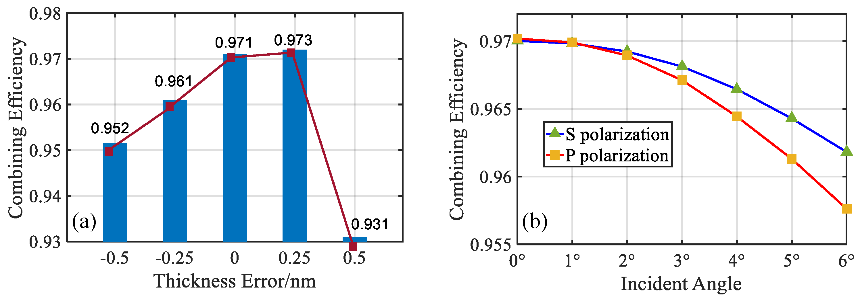
3.2. Effect of the Filter Optical Characteristics on the Combining Efficiency
3.3. Effect of the Filter Surface Roughness on the Combined Beam Quality
3.3.1. The Ideal Gaussian Beam
3.3.2. The Multimode Gaussian Beam
4. Conclusions
Author Contributions
Funding
Acknowledgments
Conflicts of Interest
References
- Wirth, C.; Schmidt, O. 2 kW incoherent beam combining of four narrow-linewidth photonic crystal fiber amplifiers. Opt. Express 2009, 17, 1178–1183. [Google Scholar] [CrossRef]
- Zervas, M.N.; Codemard, C.A. High power fiber lasers: A Review. IEEE J. Sel. Top. Quantum Electron. 2014, 20, 0904123. [Google Scholar] [CrossRef]
- Limpert, J.; Röser, F. The rising power of fiber lasers and amplifiers. IEEE J. Sel. Top. Quantum Electron. 2007, 13, 537–545. [Google Scholar] [CrossRef]
- Jauregui, C.; Otto, H.J. Optimizing high-power Yb-doped fiber amplifier systems in the presence of transverse mode instabilities. Opt. Express 2016, 24, 7879–7892. [Google Scholar] [CrossRef] [PubMed]
- Cherif, R.; Zghal, M. Characterization of stimulated Brillouin scattering in small core microstructured chalcogenide fiber. Opt. Commun. 2012, 285, 341–346. [Google Scholar] [CrossRef]
- Loranger, S.; Lambin-Iezzi, V. Stimulated Brillouin scattering in ultra-long distributed feedback Bragg gratings in standard optical fiber. Opt. Lett. 2016, 41, 1797–1800. [Google Scholar] [CrossRef] [PubMed]
- Li, Q.; Zhang, H. Stimulated Raman scattering threshold for partially coherent light in silica fibers. Opt. Express 2015, 23, 28438–28448. [Google Scholar] [CrossRef] [PubMed]
- Sophie, A.; Patrick, M. Thermal effects on the photoelastic coefficient of polymer optical fibers. Opt. Lett. 2016, 41, 2517–2520. [Google Scholar] [CrossRef] [PubMed]
- Mallek, D.; Kellou, A. Instabilities in high power fiber lasers induced by stimulated Brillouin scattering. Opt. Commun. 2013, 308, 130–135. [Google Scholar] [CrossRef]
- Schmidt, O.; Wirth, C. Spectral beam combination of fiber amplified ns-pulses by means of interference filters. Opt. Express 2009, 17, 22974–22982. [Google Scholar] [CrossRef]
- Chen, F.; Ma, J. Coupling efficiency model for spectral beam combining of high-power fiber lasers calculated from spectrum. Appl. Opt. 2017, 56, 2574–2579. [Google Scholar] [CrossRef]
- Regelskis, K.; Hou, K. Spatial dispersion-free spectral beam combining of high power pulsed Yb-doped fiber lasers. In Proceedings of the Conference on Lasers and Electro-Optics/Quantum Electronics and Laser Science Conference and Photonic Applications Systems Technologies, San Jose, CA, USA, 4–9 May 2008. [Google Scholar]
- Eastman, J.M. Scattering by all-dielectric multilayer bandpass filters and mirrors for lasers. Phys. Thin Films 1978, 10, 167. [Google Scholar]
- Born, M.; Wolf, E. Principles of Optics: Electromagnetic Theory of Propagation, Interference and Diffraction of Light; Elsevier: Amsterdam, The Netherlands, 2013. [Google Scholar]
- Meinel, K.; M Schindler, K. Scanning tunneling microscopy study on the preparation and characterization of zirconium oxide islands on Ag (100). Surf. Sci. 2002, 515, 226–234. [Google Scholar] [CrossRef]
- Vidal, B.; Vincent, P. Metallic multilayers for x rays using classical thin-film theory. Appl. Opt. 1984, 23, 1794–1801. [Google Scholar] [CrossRef]
- Prudnikov, I.R. Theoretical modeling of hard X-ray surface modes in a periodic multilayer. Opt. Commun. 2008, 281, 113–120. [Google Scholar] [CrossRef]
- Kim, D. The influence of Au thickness on the structural, optical and electrical properties of ZnO/Au/ZnO multilayer films. Opt. Commun. 2012, 285, 1212–1214. [Google Scholar] [CrossRef]
- Bennett, H.E.; Porteus, J.O. Relation between surface roughness and specular reflectance at normal incidence. JOSA 1961, 51, 123–129. [Google Scholar] [CrossRef]
- Tabatabaeenejad, A.; Moghaddam, M. Bistatic scattering from three-dimensional layered rough surfaces. IEEE Trans. Geosci. Remote Sens. 2006, 44, 2102–2114. [Google Scholar] [CrossRef]
- Brown, G.C.; Celli, V. Vector theory of light scattering from a rough surface: Unitary and reciprocal expansions. Surf. Sci. 1984, 136, 381–397. [Google Scholar] [CrossRef]
- Carniglia, C.K. Scalar scattering theory for multilayer optical coatings. Opt. Eng. 1979, 18, 104–115. [Google Scholar] [CrossRef]
- Hou, H.; Shen, J. Stratified-Interface Scattering Model for Multilayer Optical Coatings. Acta Opt. Sin. 2006, 26, 1102. [Google Scholar]
- Chen, F.; Ma, J. 10 kW-level spectral beam combination of two high power broad-linewidth fiber lasers by means of edge filters. Opt. Express 2017, 25, 32783–32791. [Google Scholar] [CrossRef]
- Kaiser, T.; Flamm, D. Complete modal decomposition for optical fibers using CGH-based correlation filters. Opt. Express 2009, 17, 9347–9356. [Google Scholar] [CrossRef]
- Schmidt, O.A.; Schulze, C. Real-time determination of laser beam quality by modal decomposition. Opt. Express 2011, 19, 6741–6748. [Google Scholar] [CrossRef]
- Schulze, C.; Naidoo, D. Wavefront reconstruction by modal decomposition. Opt. Express 2012, 20, 19714–19725. [Google Scholar] [CrossRef]


© 2019 by the authors. Licensee MDPI, Basel, Switzerland. This article is an open access article distributed under the terms and conditions of the Creative Commons Attribution (CC BY) license (http://creativecommons.org/licenses/by/4.0/).
Share and Cite
Ma, J.; Chen, F.; Wei, C.; Zhu, R. Modeling and Analysis of the Influence of an Edge Filter on the Combining Efficiency and Beam Quality of a 10-kW-Class Spectral Beam-Combining System. Appl. Sci. 2019, 9, 2152. https://doi.org/10.3390/app9102152
Ma J, Chen F, Wei C, Zhu R. Modeling and Analysis of the Influence of an Edge Filter on the Combining Efficiency and Beam Quality of a 10-kW-Class Spectral Beam-Combining System. Applied Sciences. 2019; 9(10):2152. https://doi.org/10.3390/app9102152
Chicago/Turabian StyleMa, Jun, Fan Chen, Cong Wei, and Rihong Zhu. 2019. "Modeling and Analysis of the Influence of an Edge Filter on the Combining Efficiency and Beam Quality of a 10-kW-Class Spectral Beam-Combining System" Applied Sciences 9, no. 10: 2152. https://doi.org/10.3390/app9102152
APA StyleMa, J., Chen, F., Wei, C., & Zhu, R. (2019). Modeling and Analysis of the Influence of an Edge Filter on the Combining Efficiency and Beam Quality of a 10-kW-Class Spectral Beam-Combining System. Applied Sciences, 9(10), 2152. https://doi.org/10.3390/app9102152