Enhanced Application of Principal Component Analysis in Machine Learning for Imputation of Missing Traffic Data

Abstract

Missing value imputation approaches have been widely used to support and maintain the quality of traffic data. Although the spatiotemporal dependency-based approaches can improve the imputation performance for large and continuous missing patterns, additionally considering traffic states can lead to more reliable results. In order to improve the imputation performances further, a section-based approach is also needed. This study proposes a novel approach for identifying traffic-states of different spots of road sections that comprise, namely, a section-based traffic state (SBTS), and determining their spatiotemporal dependencies customized for each SBTS, for missing value imputations. A principal component analysis (PCA) was employed, and angles obtained from the first principal component were used to identify the SBTSs. The pre-processing was combined with a support vector machine for developing the imputation model. It was found that the segmentation of the SBTS using the angles and considering the spatiotemporal dependency for each state by the proposed approach outperformed other existing models.

1. Introduction

A traffic state of congestion generally arises at the sites that have traffic volume exceeding the associated road capacity. The traffic congestion induces inefficiencies that cause excessive travel time, energy consumption and emission of greenhouse gases. In order to address this problem, departments of transportation (DOTs) and other authorities spend significant portions of their budgets on intelligent transportation system (ITS) applications to monitor traffic flows and manage congestion-related issues. Data collected from stationary detectors including loop detectors are most widely used for monitoring the traffic conditions. Although the ITS applications ideally need complete and continuous streams of traffic data in order to function properly, in reality, significant portions of the collected data from the loop detectors are often missing, causing flaws potentially resulting in under or overshooting errors with existing prediction models for ITS applications [1,2,3,4]. For example, Qu et al. [5] report that roughly 10% of daily traffic volume data is missing in Beijing, China, mainly due to malfunctions of detectors. Nguyen and Schere [6] point out that about 25% to 30% of the traffic detectors managed by the Virginia Department of Transportation are offline at any given time.

There are different categories of imputation methods. They are historical (neighboring), spline/regression, matrix-based, and non-parametric methods. The historical method recovers the missing portion of traffic data based on the data collected at the same location from neighboring days or an average of adjacent locations [7,8]. According to Qu et al. [5], the historical imputation method cannot guarantee that the data include all the traffic flow patterns that vary from day to day, even if a large amount of the data has been collected. The spline/regression approach estimates the missing data by applying mathematical interpolations utilizing the neighboring spatiotemporal data on the same day [9,10]. According to Boyles [11], the historical and spline/regression approaches are structurally simple and hence less demanding on computational resources while providing opportunities for intuitive interpretations of data. A matrix-based imputation method models traffic data by a matrix which can contain more information, including traffic patterns, than vectors and has been initially introduced by Qu et al. [5,12]. They proposed the Bayesian principal component analysis and probabilistic principal component analysis (PPCA) for imputing incomplete traffic-flow volume data. These imputation methods have outperformed other conventional methods in terms of effectiveness and accuracy, and show superior imputation performances when the missing patterns are randomly distributed. However, Tan et al. [13] mention that the existing methods do not work well when the proportion of the missing data gets larger including some extreme cases of dealing with multiple days’ worth of missing data.

Another approach for missing value imputation is non-parametric modeling. The general structure of the non-parametric model is not predefined and therefore obtained from historical data. “Non-parametric” implies that the number of parameters and their typology is unknown prior to the application. The main advantage of this model is that they can handle complex and non-linear structures. There are many variations of the non-parametric model including, artificial neural networks (ANN), decision trees, k-nearest neighbor (KNN) and support vector regression (SVR). Most machine learning (ML) methods can be considered as non-parametric models. Several researchers have identified non-parametric modeling as a flexible approach for imputations of missing traffic data [14].

The spatial and temporal correlation-aspects based on the actual relationship have been employed with matrix-based or non-parametric imputation methods to solve the large-data missing problems [3,13,14,15,16]. However, the previous studies have a common limitation that they did not explicitly consider the traffic states and their changes, and this can deteriorate the imputation performances.

Traffic data are inevitably affected significantly by the traffic state, e.g., free flow state vs. congested traffic state. The traffic flow data in the same traffic state are the results of being exposed to similar conditions. When the data are from different states, they show significantly different patterns. Especially congested state and transition state show more complex patterns than the free flow state. Because the phenomenon of the traffic congestion usually propagates up-stream with their associated traffic states, and it lasts for a relatively long time period, the data from neighboring detectors can be utilized for representing the traffic state of a missing target. Bottleneck activation and derived shockwaves are the most common examples. Thus, the spatial and temporal considerations of traffic states for identifying complex traffic conditions can improve imputation accuracies.

Generally, previous studies have focused on the traffic state of a single spot, and therefore it cannot be applied for missing value imputations for the target area with the missing data. A section-based identification of traffic states that utilizes the neighboring detector’s data (excluding the missing data at the target) is needed to improve the performance of missing value imputation.

The objective of this study is to propose a new approach for the imputation of missing data by identifying section-based traffic state (SBTS) of a target location, and determining tempo-spatial dependencies customized for each SBTS, with data at different time periods from upstream/downstream traffic detectors in the vicinity of the target. A principal component analysis (PCA) can be used in two ways with relatively simple and light mathematical operations for practical implementations in the field. First, the angle between the first principal component (PC) and the standard vector is calculated. The angle can be used not only to classify the SBTS but it can also be used as an independent variable. Second, the PC loading is applied for variable selection to reflect the spatiotemporal dependencies among variables for each SBTS. The imputation models are developed for each SBTS using a regression model of the support vector machine (SVM). The performance of the SBTS separation of the proposed angle is compared with the average speed by using the speed-flow plot. The imputation performance of the proposed imputation method is compared with some relevant methods, such as linear interpolation, artificial neural network, and k-nearest neighborhood method, against the missing data rate of 10%, 20%, and 30%.

The remainder of this study consists of four sections. The next section provides the theoretical background of the PCA and its application for determining SBTSs and missing value imputations. The SVM for the imputation model is also described. The third section describes the study data. The fourth section provides the result of the proposed model and evaluations. Then the conclusion section follows.

2. Methods

2.1. Principal Component Analysis

The PCA is a multivariate analysis technique that transforms correlated variables into a few independent principal components that represent most of the information of the original data [17]. In the 1930s, Hotelling designated low-level independent factors as components and named the approach as PCA because it is sequentially maximizing the contribution of each component to the variance of the original variables. When the overall average of the data set is 0, the first principal component $w_1$ of the data set X is defined as follows [18].

$$w_1=\arg \underset{\Vert w\Vert =1}{\max }E\{{(w^{T}X)}^2\}$$

(1)

To find the $k$-th principal component, we used $\widehat{X_k}$ to eliminate $k-1$ principal components in $X$.

$$\widehat{X_k}=X-{\displaystyle \sum }_{i=1}^{k-1}{w}_i{w}_i^{T}X$$

(2)

$$w_k=\arg \underset{\Vert w\Vert =1}{\max }E\{{(w^T\widehat{X_k})}^2\}$$

(3)

This maximization problem was solved by the Lagrangian method and the result was equivalent to finding eigenvalues and eigenvectors. The magnitude of variance was equivalent to the size of eigenvalue. In the PCA, samples of higher dimensional space transformed into samples of lower dimensional space (principal component) without dependencies by using orthogonal transformations. The first principal component had the greatest variance and the PCs were orthogonal because they were eigenvectors of the symmetric (covariance or correlation) matrix [17].

2.2. Angle for SBTS

As described earlier, the PC was the linear combination of the variables and the first PC was the linear axis that held the largest variance. The direction of the first PC depended on a given data set, and the degree of its fluctuations/variations was less affected by the robust aspect of PCA [16]. This aspect was considered as one of the main advantages of the PC approach. The angle of the first PC was used to measure the SBTS of a group of the spatiotemporal speed data. The angle between the first PC and the standard vector, $v_s$ = [1, 1, 1, ...], at a time $t$, $An{g}_t$ was calculated by the following equation, where $w_1$ is the first PC.

$$An{g}_t=Arccos\left(\frac{w_1·v_s}{\left|w_1\right|·\left|v_s\right|}\right)$$

(4)

Fang et al. [19] used this angle for making real-time crash predictions. They have extracted eigenvectors from traffic speed, occupancy, and flow data. The eigenvectors are independent of each other, and it was possible to avoid the multicollinearity between the loop data.

In order to illustrate the proposed concept for identifying SBTSs, a simulated numerical example has been employed. It was assumed that there were eight consecutive stationary detectors. The gaps between the detectors were identical with the length of 1.67 km. The first downstream detector did not experience the traffic congestion because the activation point of the bottleneck was the second upstream detector. From second to sixth downstream detectors experienced two types of shockwaves, i.e., backward-forming and forward-recovery. The wave speed of the backward-forming was 20 km/h, and the wave speed of the forward-recovery was 10 km/h. The time period of a day was from 2 p.m. to 10 p.m., and the bottleneck was activated around 4 p.m. and deactivated at around 8 p.m. The speed of the free flow state was 80 km/h, and the congested state was 15 km/h. The speed data were combined with the noise of the standard normal distribution with a standard deviation of 8 km/h. The $An{g}_t$ calculated with the speed data and the speed contour-plot is shown in Figure 1. The change of the $An{g}_t$ is shown clearly according to the evolution of traffic congestion. The $An{g}_t$ can be used to divide the SBTS of the study area and also used as an independent variable for the imputation model.

2.3. Spatiotemporal Dependence

The variable selection can improve the imputation performance when the problem of over-fitting arises. Machine learning techniques have normally faced the problem of over-fitting. The variable selection can be implemented using the spatiotemporal dependence of the variables that can be identified using the structure of the variables. The variable structures were identified by using the factor-loading which indicated the individual contribution of each variable to the PC [17]. If the symmetric matrix, covariance matrix or the correlation matrix, was used for PCA, the variables were grouped independently because the PCs were independent of each other. However, since one variable was not loaded on one PC, a simple structure that allowed easy handling was obtained using an appropriate rotation. The simple structure implied that each variable had a high loading on one factor and very low loadings on the other factor [20]. The simple structure was applied to an SBTS in which one variable can exert influences on only one factor. The simple structure can be obtained by a change of basis from the original PCA result, and there are rotation methods that maintain orthogonality such as Varimax or that does not such as Oblimin [20]. The choice of the rotation method depends on the applicability and appropriateness of the method for the desired applications.

The Varimax was used as an orthogonal basis to simplify the subspace without changing the actual coordinate system. It is a rotation used when the PCA is hard to analyze due to the dense result. The Varimax uses an objective function that allows a given variable to be loaded heavily on a single PC and to maximize the overall variance. The objective function is as follows [20].

$$P\mathit{Varimax}=\mathit{arg}\underset{P}{\mathit{max}}{\left\{\frac{1}{p}{{\displaystyle \sum }}_{j=1}^k{{\displaystyle \sum }}_{i=1}^p{\left(\Lambda P\right)}_{ij}^4-{{\displaystyle \sum }}_{j=1}^k\frac{1}{p}{{\displaystyle \sum }}_{i=1}^p{\left(\Lambda P\right)}_{ij}^2\right\}}^2$$

(5)

By using Varimax rotation, the basis was transformed and the variables were assigned to a PC with the highest loading. It was eligible for grouping variables based on their independencies while the grouped variables were dependent on each other. Several PCs can be selected according to the cumulative loadings of the target variable [20].

2.4. Support Vector Machine and Regression

The SVM is one of the well-known machine learning techniques and has the advantage of its generalizing ability and having the optimal global solution, due to the fact that it uses the principle of minimizing the structural risk (maximum margin), unlike the neural network which adopts the empirical risk minimization principle (minimize residual) [21,22].

The SVM is also suitable for complex systems and has robust performance when processing corrupted data. The SVM is a classifier that maximizes the margin, the distance between support vectors. A support vector is a data element closest to the hyperplane in multidimensional space. The SVM generates hyperplanes in high density or spaces with infinite dimensions in which data analyses such as classification or regression can be conducted [22]. The excellent separation is achieved by the hyperplane that is the longest distance from the closest training data point of a class, since the larger the margin, the lower the generalization error of the classifier [23,24,25].

Let $w$ be a normal vector, $y_i$ is a variable that indicates the group to which $x$ belongs by 1 and −1, and $b$ is the distance from the point where $x$ is projected to $w$. In this case, the hyperplane satisfying $w·x-b\ge 1$ (when $y_i=1$) or $w·x-b\le -1$ (when $y_i=-1$) is the line passing through the support vector [22]. Since there is no other data between these distances (hard margin), the following constraints and object function are expressed.

$$\mathit{arg}\underset{\left(w,b\right)}{\mathit{min}}\Vert w\Vert$$

(6)

$$subjectto{y}_i\left(w·x-b\right)\ge 1$$

(7)

The objective function is a problem of finding the norm of the normal vector, which is a problem of finding the square root. The Lagrange multiplier can be used to find the saddle point as in the following and this is solved by partial differential equations [22]. The SVM permits soft margins that allow some classification error to avoid over-fitting. A misclassification tolerance term ${\xi }_i$ is added to the objective function ([21], Chapter 8).

$$\underset{\left(w,b\right)}{min}{\Vert w\Vert }^2+C{\displaystyle \sum }_{i=1}^n{\xi }_i$$

(8)

$$subjectto{y}_i\left(w·x-b\right)\ge 1-{\xi }_i$$

(9)

The SVM uses a kernel trick that replaces the calculation of the inner product of the vector with the kernel function to reflect the nonlinearity [23]. Linear classification was performed at the modified high dimension, but nonlinear classification was performed in the original space. There were Linear, polynomial, and radial basis kernel function, and this study used a radial basis function. The support vector regression, which is a regression model using SVM, can be expressed as below using the soft margin. $\mathsf{\Gamma }$ is the cost function [25].

$$f(x)=C{\displaystyle \sum _{i=0}^l\mathsf{\Gamma }(f(x_i-y_i))+{\Vert w\Vert }^2}$$

(10)

The partial differential is $w={\displaystyle \sum }_{i=0}^l\left({\alpha }_i-{\alpha }_i{}^{*}\right)\Phi \left(x_i\right)$. As a consequence, the $f\left(x\right)$ is ${\displaystyle \sum }_{i=0}^l\left({\alpha }_i-{\alpha }_i{}^{*}\right)\left(\Phi \left(x_i\right)·\Phi \left(x\right)\right)+b$. The dot product of $\left(\Phi \left(x_i\right)·\Phi \left(x\right)\right)$ can be replaced by the kernel function, and it is as in the following [23]. This study used a radial basis kernel function as used in Wu [26] for traffic data.

$$f\left(x\right)={\displaystyle \sum }_{i=0}^l\left({\alpha }_i-{\alpha }_i{}^{*}\right)k\left(x_i,x_i\right)+b$$

(11)

3. Study Data

The Gyeongbu Expressway in South Korea was taken as the study site. Our study section was approximately 12.6 km in length in the vicinity of the Greater Seoul Area (GSA), with 12 vehicle detection systems (VDSs). The geographical information, the number of VDSs, and the absolute and relative milepost (unit is km) are shown in Figure 2. Traffic speed-data were collected from the Korea Expressway Corporation. The speed-data of each VDS was collected at the 5-min aggregate level. The observation period was between 1 March 2016 and 31 August 2016. All data were from real-life operations and the total number of days used was 158 days.

The proposed model was developed using the speed-data from the neighboring VDS at the seven-time steps of the imputation variable, i.e., three-time steps of the past and future respectively in addition to a current time step. Since there were speed-data in 12 detectors at seven-time steps, there were 84 spatiotemporal variables as independent variables when there was no missing value. The missing data patterns in this study used a missing at determinate (MD) approach. The MD was known to be one of the difficult patterns of missing data for the matrix-based imputation methods to solve. The MD strategy implied that the missing traffic data have specific patterns. The patterns were normally caused by the long-term malfunctioning of the detectors and the detectors were no longer useful [27]. When the MD strategy was applied, there were 77 spatiotemporal variables as independent variables. The training data were arbitrarily divided into 70%, 80%, and 90%. The training dataset had no missing data but the validation dataset had missing data with the MD strategy.

4. Analysis

4.1. SBTS Identification

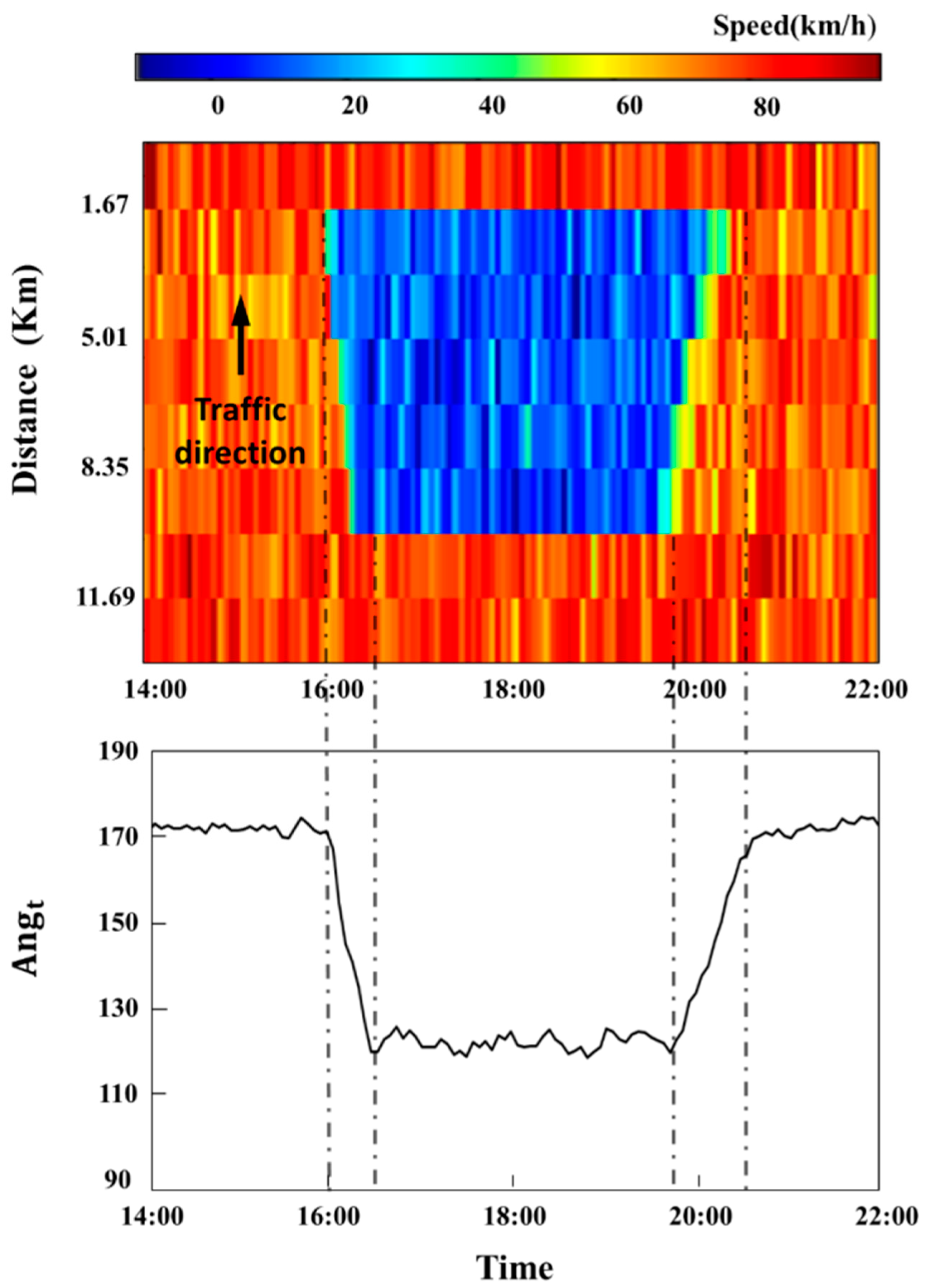
The $An{g}_t$ was calculated using the speed data and the results are shown in Figure 3. The figure shows the speed-contour plot on 3rd March 2016 in the test site and the plot of the $An{g}_t$ from the same day. The bottleneck was normally activated at number 3 and the queue tail occurred near number 9. As described in the methods section, the $An{g}_t$ plot had a similar pattern with the speed-contour plot in the real traffic data. The $An{g}_t$ represented a whole SBTS as opposed to the prediction approach based on spot-based traffic states which had a major limitation of being unable to operate when the data was missing. The $An{g}_t$ indicated the degree of the congested area in the section. The low $An{g}_t$ value represented the spread of congestion over a larger range of road sections in the study area. In addition, the speed of the evolution of traffic congestion can be interpreted by the angle. When the evolution of traffic congestion started rapidly, $An{g}_t$’s inclination was steep. On the other hand, when the evolution of traffic congestion started smoothly, $An{g}_t$’s inclination was also smooth.

Many researchers have divided traffic flows into several different transitional states with their own criteria to identify traffic flow characteristics. Wu [26] proposed finer classifications of SBTSs based on the fundamental diagrams. The free flow was further divided into the SBTSs of free fluid traffic and bunched fluid traffic. The congested section state was further classified into bunched congested traffic and standing congested traffic. In the 2010 edition of the Highway Capacity Manual [28], the traffic flow of the freeway was classified into six different SBTSs based on traffic densities. Noroozi and Hellinga [29] divide SBTSs using a speed-occupancy graph. They proposed the boundary lines on the graph, which can divide the SBTS into two free flow, congestion and transition SBTSs. The existing methods on SBTS identification were suitable when complete data were available because they considered spot-based traffic states. However, the identification of the SBTSs was needed for the missing value imputation due to the absence of the target data. This is the reason why identifying the SBTS using $An{g}_t$ is critical for missing value imputations.

In this study, three traffic states were considered. The SBTS I contained the traffic state of all spots that were in the free flow state. The SBTS II was the traffic condition of the section that the queue length in the analyzed site was near the empirical maximum and did not expand anymore. SBTS III was between I and II that the traffic condition of the section was either queue build-up or diminishing, e.g., backward-forming and forward-recovery shockwaves. In the empirical case, the SBTS III may contain the traffic conditions of the section where the queue is not maximized, yet maintained.

The boundaries between these states can be identified easily from diagrams as shown in Figure 3. In the study section, the SBTSs were classified into three SBTSs based on the $An{g}_t$ value measured using 12 loop detector stations. The data from 3 March 2016 showed a significant difference in terms of peak patterns between morning and evening, and the $An{g}_t$ certainly captured the difference in this degree of congestion. The results of t-tests show that the three SBTSs are all statistically different with 95% confidence levels. This verifies that $An{g}_t$ can be used as a classification index of traffic SBTS. The characteristics of the three SBTSs are defined as in the following.

• SBTS I: free flow state at all spot ($An{g}_t\ge 173$)
• SBTS II: maximized queue ($An{g}_t\le 165$)
• SBTS III: between I and II ($173\ge An{g}_t\ge 165$).

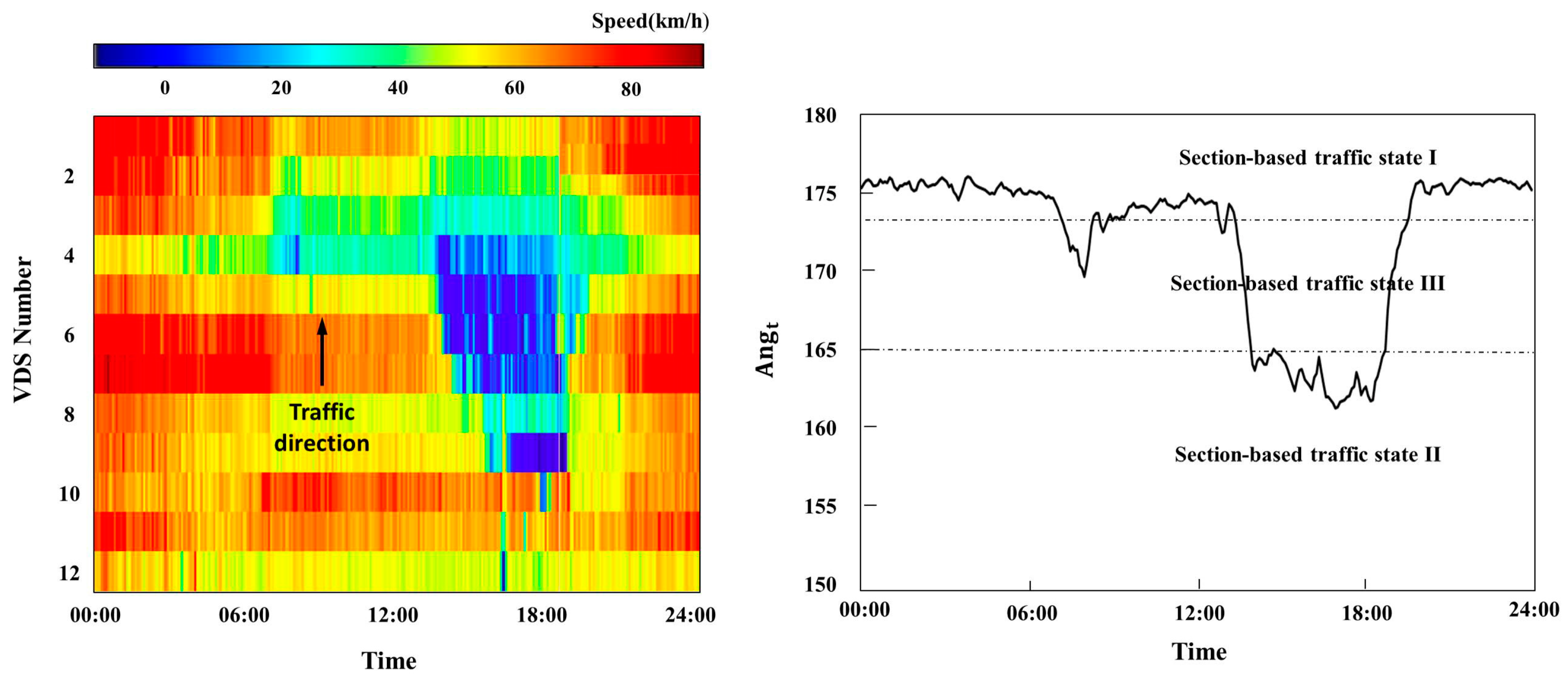
The classification performance of the SBTSs using the $An{g}_t$ was compared with that of using the average speed. Figure 4 shows that the $An{g}_t$ and average-speed plots on the 12 March 2016 when the two peak congestions in the morning and evening typically occurred. As can be seen, the overall patterns of the two plots were similar during the period of changing SBTSs. In the second congestion, however, the identified points in time that the congestion section state changed into the free flow section state and were different among the two indices. The congestion recovery time using the average-speed showed a later time than that of using the $An{g}_t$.

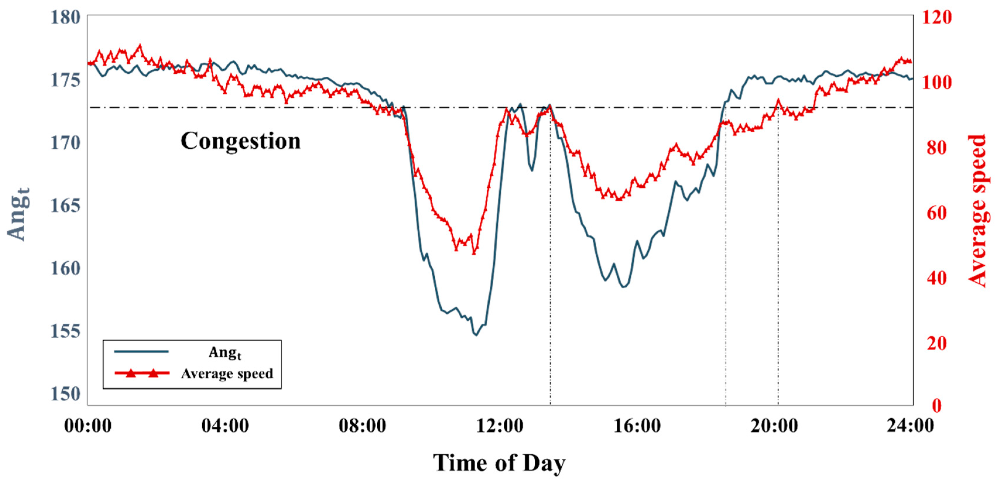
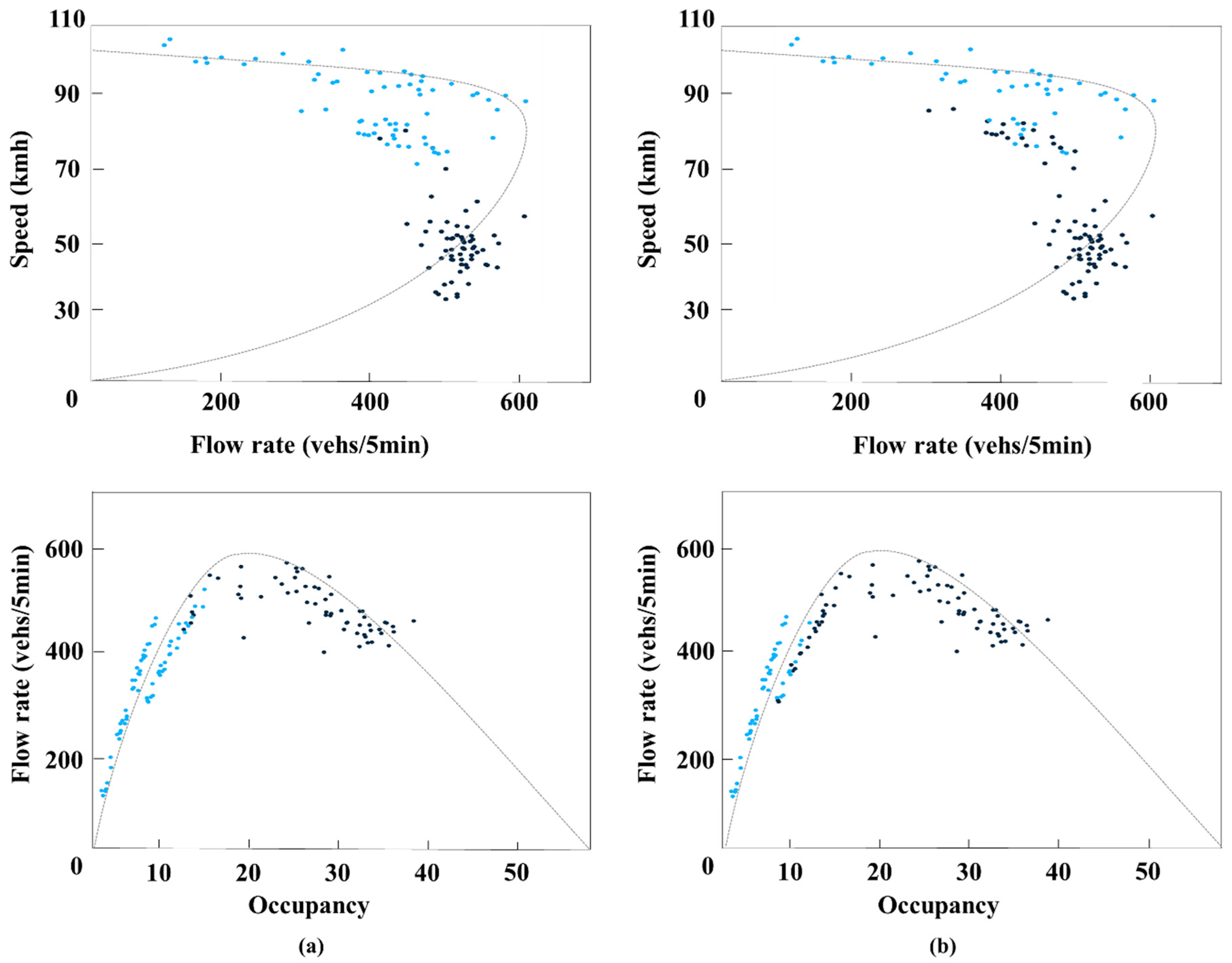
In order to compare the classification performances with respect to the theoretical congestion, Figure 5 shows the speed-flow plot and occupancy-flow plot at the VDS 4 which was located at the front of the congestion queue. To clarify the difference of the average speed and $An{g}_t$, the time period of Figure 5 was set from 13:30 p.m. to 24:00 p.m. in the figure. The black dots indicate that the SBTS of VDS 4 was under a congestion section state. Figure 5a shows the classification using the $An{g}_t$ and Figure 5b shows the classification using the average speed. The congestion section states identified by $An{g}_t$ and the distribution of black dots in the plots of Figure 5a are mostly matched with the theoretical congestion section state described in Highway Capacity Manual [28]. As described by May [30] and other many related studies, the upper regime of the speed-flow plot is described as the free-flow section state and the lower regime is referred to as the congestion section state. Under the free-flow section state, the speed decreases as the flow increase up to the maximum flow. When the flow reached the maximum flow (capacity), which occurred mostly at the inflection point, further speed reduction, coupled with flow-reductions, began. The lower regime of the plots mostly depicts the congestion section state. The congestion section state identified by the average speed, and the distribution of black dots in the plots of Figure 5b, however, are not matched well for theoretical congestion or for a free-flow section state. From these empirical results, it is shown that using $An{g}_t$ for classifying SBTS based on the traffic flow theory is better than the average-speed approach.

4.2. Spatiotemporal Dependence of SBTS

In order to identify the spatiotemporal dependencies of the variables, the PCA was carried out with the Varimax rotation using the training data set that has the value of imputation target. The variables were clustered by the PCs that had the most loading of a variable. The PC was independent from other PCs and had several highly loaded variables. The variable dependence on the imputation target was identified by the accumulated loadings of the target variable on the PCs. The threshold of 0.95 was used in this study.

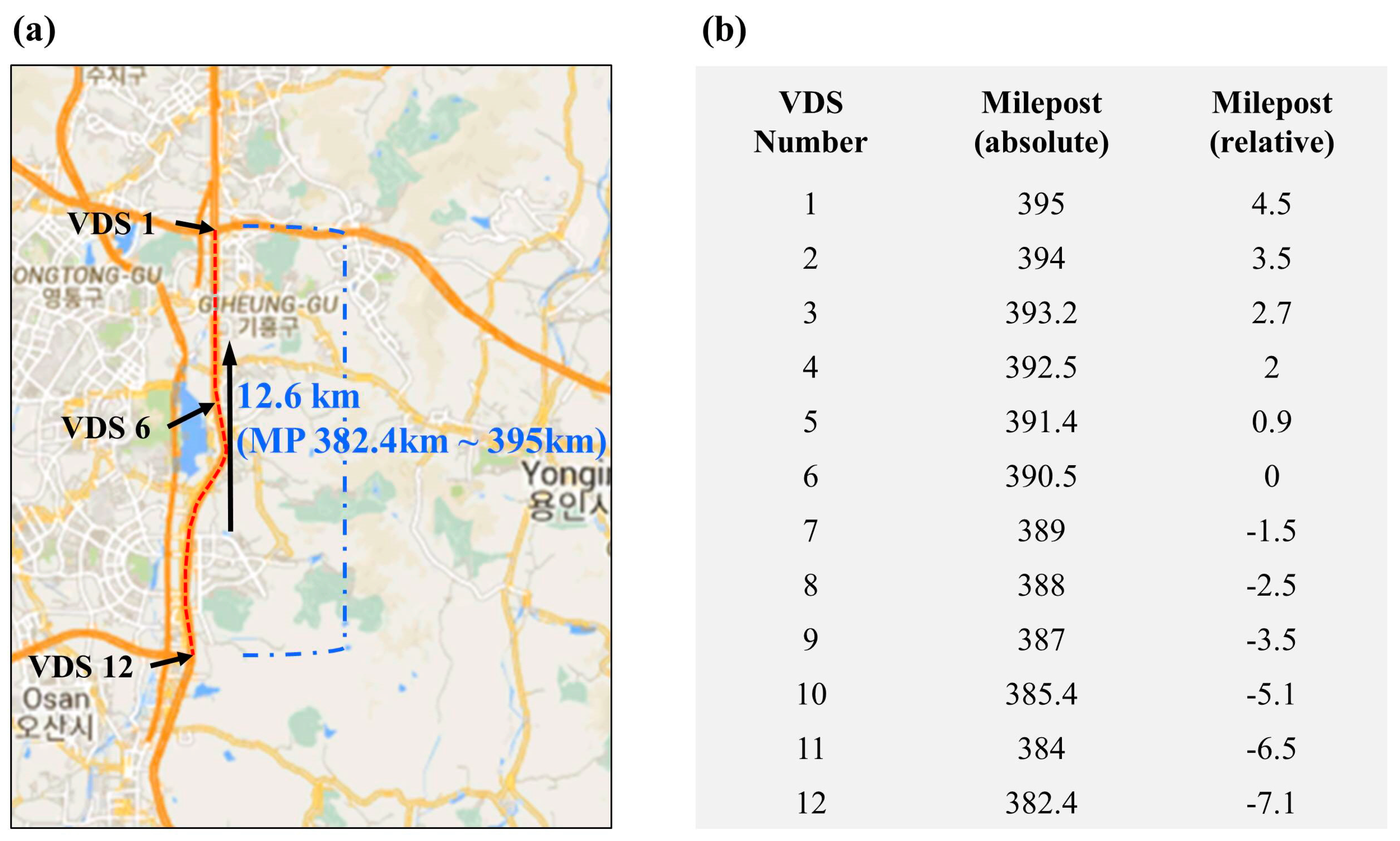
The results of the spatiotemporal dependence between the target detector and surround detectors are shown in Figure 6. The numbers in Figure 6 are the numbers of the detector as in Figure 2 and the notation of Tk is the time slice of the k-minute. The imputation target in this study was chosen to be and referred to as the detector number 6 because it was located roughly in the middle of the queue. As described earlier, the head of the queue was at number 3 and the tail was at number 9. As seen in Figure 6, almost all of the independent variables of the SBTS I were included in the loading of less than 0.95 and were not found with any specific patterns. On the other hand, the SBTS of main interests for congestion management, SBTS II and III, showed unique patterns. The SBTS II’s spatiotemporal dependence was constructed by the nearest up- and down-stream detectors, the detectors near the bottleneck activation point, and the most upstream point of the study area. The SBTS III’s spatiotemporal dependence was constructed by only the nearest up- and down-stream detectors. As a result, the spatiotemporal dependencies on the imputation target are different for each SBTS and can represent the characteristics of each SBTS.

Note that, in this study, the suggested method has been applied for the imputation of existing historical data and tested. However, theoretically, it can be directly used for estimating the missing values in a real-time environment by changing the input variables only. In the regression model, instead of the time window [${\mathrm{T}}_{-15}$~${\mathrm{T}}_{+15}$] shown in Figure 6, the dependent variables can have a time window of [${\mathrm{T}}_{-30}$~${\mathrm{T}}_0$].

4.3. Imputation Performance

To check and compare the performance of the proposed model, five test-case scenarios were set up as shown in

Table 1. Description of cases for empirical analysis.

Case	Variables	Segmentation of SBTS	Using Angt *
Case 1	All	No	No
Case 2	All	Yes	No
Case 3	All	Yes	Yes
Case 4	Selected	Yes	No
Case 5	Selected	Yes	Yes

* The angle between the first PC and the standard vector $v_s$ at a time $t$.

. In this test, the performance measure used was the root mean squared error (RMSE). Where y_e^(m) is the estimated value and y_r^(m) is the observed value, respectively, whereas $M$ denotes the total number of testing entries we used.

$$RMSE=\sqrt{\frac{1}{M}{\displaystyle \sum }_{m=1}^M{\left(y_e^{\left(m\right)}-y_r^{\left(m\right)}\right)}^2}$$

(12)

As stated, the missing target was detector number 6 with the MD strategy that assumed malfunctions for all observation days in the validation dataset. All speed data of the number 6 in the validation data were removed. The $An{g}_t$ was newly computed from the validation data, which did not include VDS 6 traffic-speed data. The comparison of the imputation performances especially in SBTSs II and III were of great interest for congestion management.

The results of the performance comparisons when the training data and validation data were 80% and 20% respectively among the SVR-based cases, as shown in

Table 2. Validation results of empirical analysis.

Model	RMSE * (km/h) of Validation
	SBTS II	SBTS III	Aggregate
case 1	12.586	11.696	12.173
case 2	11.607	11.961	11.785
case 3	11.564	11.902	11.733
case 4	11.019	11.222	11.120
case 5	11.070	11.072	11.071

* Root mean squared error.

. There were some key findings. First, the model segmentation by using the $An{g}_t$ improved the performance and this was supported by the RMSE difference between Case 1 and Case 2. The rest of the comparisons were conducted to examine the effects of (i) the variable selection and (ii) the addition of the angle to the independent variables, and the standard model segmentation was applied afterwards. Second, the variable selection considering the factor loading improved the imputation performance. The evidence is visible from the RMSE differences between Case 2 and Case 4, and Case 3 and Case 5. Third, the use of the angle as an independent variable improved the imputation performance except when the variable selection was used in the SBTS II. This is supported by the RMSE differences between Case 2 and Case 3, and Case 4 and Case 5. The range of the computation time of the proposed approach for all cases was from 6 s to 27 s, and it is reasonable for actual implementations in the field for practitioners at DOTs.

The imputation performances of the comparison method according to the missing rate of 10%, 20%, and 30% are shown in

Table 3. Comparison result according to missing ratio.

(a) Missing ration 10%
Model	RMSE (km/h) of Validation (Percentage Difference)
	SBTS II	SBTS III	Aggregate
Linear Interpolation	13.501 (36.5%)	15.276 (39.7%)	14.542 (38.5%)
ANN	11.102 (12.2%)	12.745 (16.5%)	12.068 (14.9%)
KNN	16.263 (64.4%)	16.352 (49.5%)	16.314 (55.4%)
Case 5	9.891	10.936	10.500
(b) Missing ration 20%
Model	RMSE (km/h) of Validation (Percentage Difference)
	SBTS II	SBTS III	Aggregate
Linear Interpolation	15.815 (42.9%)	16.165 (46.0%)	15.990 (44.4%)
ANN	12.691 (14.6%)	12.799 (15.6%)	12.713 (14.8%)
KNN	18.304 (65.3%)	17.479 (57.9%)	17.858 (61.3%)
Case 5	11.070	11.072	11.071
(c) Missing ration 30%
Model	RMSE (km/h) of Validation (Percentage Difference)
	SBTS II	SBTS III	Aggregate
Linear Interpolation	16.182 (41.7%)	15.490 (37.2%)	15.781 (39.1%)
ANN	13.494 (18.2%)	12.907 (14.4%)	13.153 (16.0%)
KNN	19.338 (69.3%)	17.851 (58.2%)	18.482 (63.0%)
Case 5	11.420	11.286	11.342

NOTE: ANN is artificial neural networks and KNN is k-nearest neighbor.

. This paper compared the performance of the proposed model against the linear interpolation method, ANN, and KNN. For the linear interpolation method, we used a nearby detector’s speed data at the same time. Before performing the ANN and KNN methods, it was necessary to determine some parameters; the number of hidden layers and the activation function for ANN and k value which is the number of neighbors for KNN. Here, we did not put much effort to apply a new or complex methodology to find optimal parameters. However, we iterated the above methods with changing parameters to find optimal parameters, which gave the minimum RMSE. In this paper, the following deterministic of the parameters was used; the number of hidden layers = 5, the activation function = linear function, and $k$ value = 83.

It was found that the proposed approach consistently improved the performance against the existing methods. Especially, the proposed model showed better performance in the SBTSs including the congested section state, which indeed was the highlight of the proposed model. In terms of the percentage differences of RMSE between the proposed method and other methods, the range was about 12.2% to 69.3%. The KNN method showed the largest difference while the ANN showed the smallest difference.

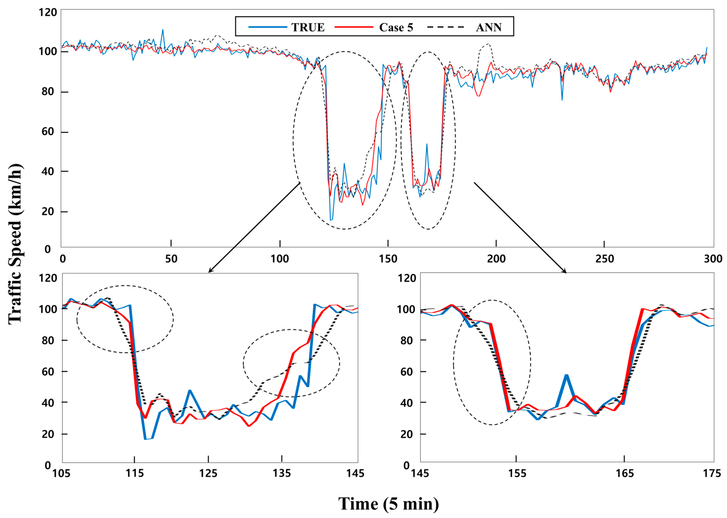
Figure 7 shows the real data and imputation results of the proposed model (Case 5) and other compared models for a particular weekday (20 July 2016). The proposed model was found to capture the precursor of transitions significantly faster. Unlike the proposed model, the two existing models with which the proposed model was compared with, tended to provide only the average value of free-flow and congestion when the transition started. This shows that it is promising to adopt the proposed approach of categorizing traffic data by each SBTS, using $An{g}_t$ and selected variables that would improve the performance of missing value imputations.

5. Conclusions and Future Work

This study proposes a novel approach of imputation of missing traffic data by identifying SBTS of a target location, and determining customized tempo-spatial dependencies for each SBTS, which consists of multiple spot-states of the desired road-section, utilizing the data from different time periods at up- and down-stream traffic detectors in the vicinity of the target area with the missing data.

The proposed $An{g}_t$-based approach more effectively divided the traffic data into different SBTS compared to the traditional average-speed approach which merely identifies states by drawing fundamental diagrams. The proposed method combined with the support vector regression, that can separate the SBTS and identify the spatiotemporal dependencies, showed consistent improvements in terms of performance of imputations. Additionally, the proposed approach showed the best performance exceeding comparison methods including linear interpolation, k-NN and ANN approaches when dealing with varying missing rates or relatively large and continuous missing patterns. The spatiotemporal dependencies detected by the method can be used as a constructive clue to identify the hidden congestion mechanism associated with the study section. In this study, the spatiotemporal dependency was widely distributed in SBTS II while it was narrowly distributed in SBTS III. The value of the $An{g}_t$ identifying the SBTS has been utilized as an input to overcome the narrow dependency in the SBTS III, and the performance of imputation has been improved.

Although the proposed approach can improve the imputation performance of missing values, and it is relatively easy to apply, there is room for further improvement. For example, the current model still requires a certain amount of historical data of the missing target in order to train with the proposed method. The directions of future research still remain to be explored. The segmentation of the SBTS in this study can branch out to various ITS applications. An automatic segmentation rule can be designed for a fluent application of the proposed approach and can be applied in the emerging data-driven ITS environments. For example, hierarchical or expectation-maximization clustering approaches using the angle value can be a near-foreseeable enhancement from this study. Furthermore, more sophisticated regression model such as deep learning models can be combined with the proposed approach to further improve the performances. Also, additional datasets can be incorporated to ensure the transferability of the proposed model.

References

1. Conklin, J.H.; Smith, B.L. The use of local lane distribution patterns for the estimation of missing data in transportation management systems. Transp. Res. Rec. 2002, 1811, 50–56. [Google Scholar]
2. Turner, S.; Albert, L.; Gajewski, B.; Eisele, W. Archived intelligent transportation system data quality: Preliminary analyses of San Antonio TransGuide data. Transp. Res. Rec. 2000, 1719, 77–84. [Google Scholar] [CrossRef]
3. Chen, C.; Kwon, J.; Rice, J.; Skabardonis, A.; Varaiya, P. Detecting errors and imputing missing data for single-loop surveillance systems. Transp. Res. Rec. 2003, 1855, 160–167. [Google Scholar] [CrossRef]
4. Smith, B.L.; Scherer, W.T.; Conklin, J.H. Exploring imputation techniques for missing data in transportation management systems. Transp. Res. Rec. 2003, 1836, 132–142. [Google Scholar] [CrossRef]
5. Qu, L.; Zhang, Y.; Hu, J.; Jia, L.; Li, L. A BPCA based missing value imputing method for traffic flow volume data. In Proceedings of the 2008 IEEE Intelligent Vehicles Symposium, Eindhoven, The Netherlands, 4–6 June 2008. [Google Scholar]
6. Nguyen, L.N.; Scherer, W.T. Imputation Techniques to Account for Missing Data in Support of Intelligent Transportation Systems Applications; Research Report UVACTS-13-0-78; University of Virginia: Charlottesville, VA, USA, 2003. [Google Scholar]
7. Afifi, A.A.; Elashoff, R.M. Missing observations in multivariate statistics I. Review of the literature. J. Am. Stat. Assoc. 1966, 61, 595–604. [Google Scholar] [CrossRef]
8. Chen, J.; Shao, J. Nearest neighbor imputation for survey data. J. Off. Stat. 2000, 16, 113. [Google Scholar]
9. Zhang, Y.; Liu, Y. Missing traffic flow data prediction using least squares support vector machines in urban arterial streets. In Proceedings of the 2009 IEEE Computational Intelligence and Data Mining, Nashville, TN, USA, 30 March–2 April 2009. [Google Scholar]
10. Al-Deek, H.M.; Venkata, C.; Chandra, S.R. New algorithms for filtering and imputation of real-time and archived dual-loop detector data in I-4 data warehouse. Transp. Res. Rec. 2004, 1867, 116–126. [Google Scholar] [CrossRef]
11. Boyles, S. Comparison of interpolation methods for missing traffic volume data. In Proceedings of the 90th Annual Meeting of the Transportation Research Board, Washington, DC, USA, 23–27 January 2011. [Google Scholar]
12. Qu, L.; Li, L.; Zhang, Y.; Hu, J. PPCA-based missing data imputation for traffic flow volume: A systematical approach. IEEE Trans. Intell. Transp. Syst. 2009, 10, 512–522. [Google Scholar] [CrossRef]
13. Tan, H.; Feng, G.; Feng, J.; Wang, W.; Zhang, Y.J.; Li, F. A tensor-based method for missing traffic data completion. Transp. Res. Part C 2013, 28, 15–27. [Google Scholar] [CrossRef] [Green Version]
14. Henrickson, K.; Zou, Y.; Wang, Y. Flexible and robust method for missing loop detector data imputation. Transp. Res. Rec. 2015, 2527, 29–36. [Google Scholar] [CrossRef]
15. Haworth, J.; Cheng, T. Non-parametric regression for space-time forecasting under missing data. Comput. Environ. Urban Syst. 2012, 36, 538–550. [Google Scholar] [CrossRef]
16. Li, L.; Li, Y.; Li, Z. Efficient missing data imputing for traffic flow by considering temporal and spatial dependence. Transp. Res. Part C 2013, 34, 108–120. [Google Scholar] [CrossRef]
17. Jolliffe, I. Principal Component Analysis; Springer: New York, NY, USA, 2011. [Google Scholar]
18. Hotelling, H. Analysis of a complex of statistical variables into principal components. J. Educ. Psychol. 1933, 24, 417. [Google Scholar] [CrossRef]
19. Fang, S.; Xie, W.; Wang, J.; Ragland, D.R. Utilizing the eigenvectors of freeway loop data spatiotemporal schematic for real time crash prediction. Accid. Anal. Prev. 2016, 94, 59–64. [Google Scholar] [CrossRef] [PubMed]
20. Costello, A.B.; Osborne, J.W. Best practices in exploratory factor analysis: Four recommendations for getting the most from your analysis. Pract. Assess. Res. Eval. 2005, 10, 1–9. [Google Scholar]
21. Vapnik, V. The Nature of Statistical Learning Theory; Springer Science & Business Media: New York, NY, USA, 2013. [Google Scholar]
22. Vapnik, V.N. An overview of statistical learning theory. IEEE Trans. Neural Netw. 1999, 10, 988–999. [Google Scholar] [CrossRef] [PubMed]
23. Gunn, S.R. Support Vector Machines for Classification and Regression; Technical Report; University of Southampton: Southampton, UK, 1988. [Google Scholar]
24. Müller, K.R.; Smola, A.J.; Rätsch, G.; Schölkopf, B.; Kohlmorgen, J.; Vapnik, V. Predicting time series with support vector machines. In Proceedings of the International Conference on Artificial Neural Networks, Lausanne, Switzerland, 8–10 October 1997. [Google Scholar]
25. Müller, K.R.; Smola, A.J.; Rätsch, G.; Schölkopf, B.; Kohlmorgen, J.; Vapnik, V. Using support vector machines for time series prediction. In Advance in Kernel Methods; Schölkopf, B., Burges, C.J.C., Smola, A.J., Eds.; MIT Press: Cambridge, MA, USA, 1999; pp. 243–253. [Google Scholar]
26. Wu, N. A new approach for modeling of Fundamental Diagrams. Transp. Res. Part A 2002, 36, 867–884. [Google Scholar] [CrossRef]
27. Little, R.J.A.; Rubin, D.B. Statistical Analysis with Missing Data, 2nd ed.; John Wiley & Sons: New York, NY, USA, 2014. [Google Scholar]
28. Transportation Research Board of the National Academics; Highway Capacity Manual: Washington, DC, USA, 2010.
29. Noroozi, R.; Hellinga, B. Real-time prediction of near-future traffic states on freeways using a Markov model. Transp. Res. Rec. 2014, 2421, 115–124. [Google Scholar] [CrossRef]
30. May, A.D. Traffic Flow Fundamentals; Prentice Hall: Upper Saddle River, NJ, USA, 1990. [Google Scholar]
Figure 1. Speed contour and A n g t plots for the numerical example.
Applsci 09 02149 g001
Figure 2. Study area in Korean freeway. (a) Geographical information. (b) Vehicle detection system (VDS) information.
Applsci 09 02149 g002
Figure 3. Speed contour and A n g t plots for empirical data on 3 March 2016.
Applsci 09 02149 g003
Figure 4. A n g t and average speed plots on 12 March 2016.
Applsci 09 02149 g004
Figure 5. Flow-speed and occupancy-flow plots at VDS 4 on March 12 2016. (a) Classified by A n g t . (b) Classified by average speed.
Applsci 09 02149 g005
Figure 6. Spatiotemporal dependence among variables (a) Section-based traffic state (SBTS) I (b) SBTS II (c) SBTS III.
Applsci 09 02149 g006
Figure 7. Traffic speed profile of real and predicted data by ANN and proposed model.
Applsci 09 02149 g007