An Improved CNN Model for Within-Project Software Defect Prediction


Abstract
1. Introduction
- We proposed an improved CNN model for better generalization and capability of capturing global bug patterns. The model learned semantic features extracted from a program’s AST for defect prediction.
- We built and published a dataset named PSC, which targeted AST-based features from the PROMISE repository based on five principles. The PSC dataset was larger than the SPSC dataset, and we excluded versions for which source code could not be found, or the labeled CSV file did not match the source code.
- We performed two experiments to validate that the CNN model could outperform the state-of-the-art machine learning models for WPDP. The first experiment demonstrated the validity of our improved model, while the second experiment validated the performance of our improved CNN model as compared with other machine learning models.
- We performed a hyperparameter search, which took dense layer numbers, dense layer nodes, kernel size, and stride step into consideration to uncover empirical findings.
- We concluded that hyperparameter instability may be a threat and an opportunity for deep learning models on defect prediction. The discovery was based on experimental data and targeted deep learning models like CNN.
2. Background
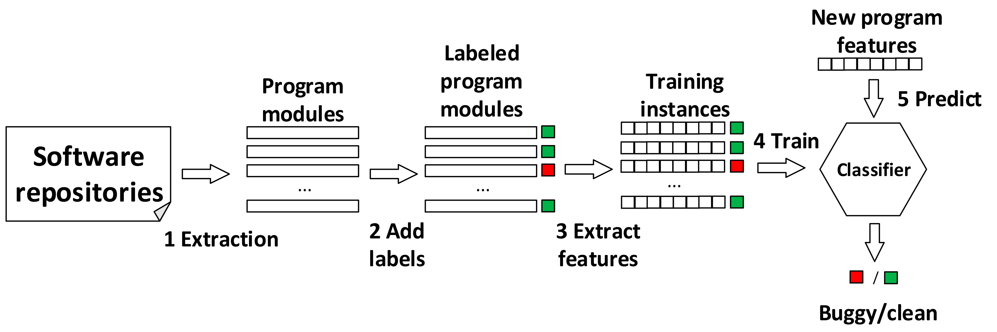
2.1. Software Defect Prediction
2.2. Convolutional Neural Network
2.3. Word Embedding
2.4. Dropout
3. Approach
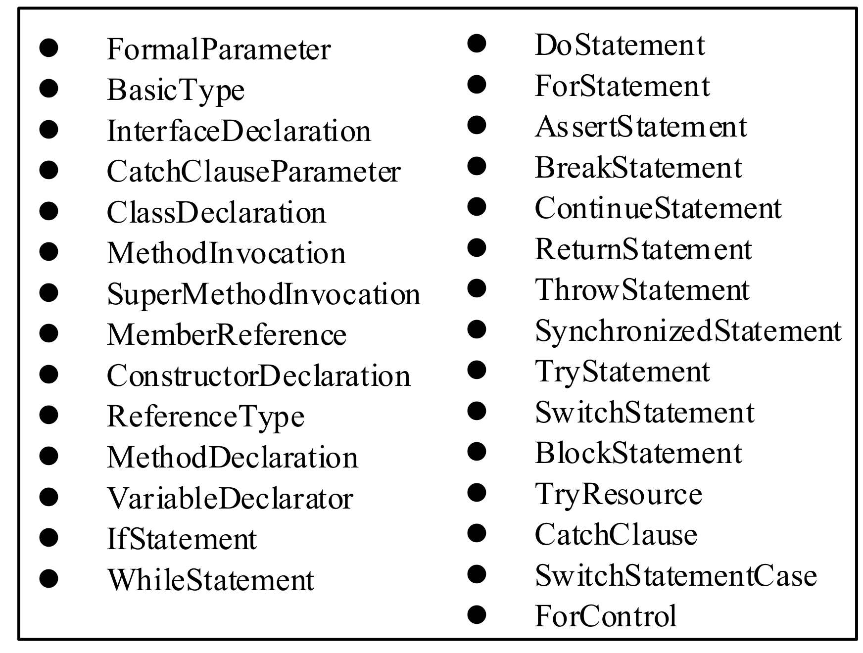
3.1. Parsing Source Code
3.2. Mapping Tokens
3.3. Handling Class Imbalance
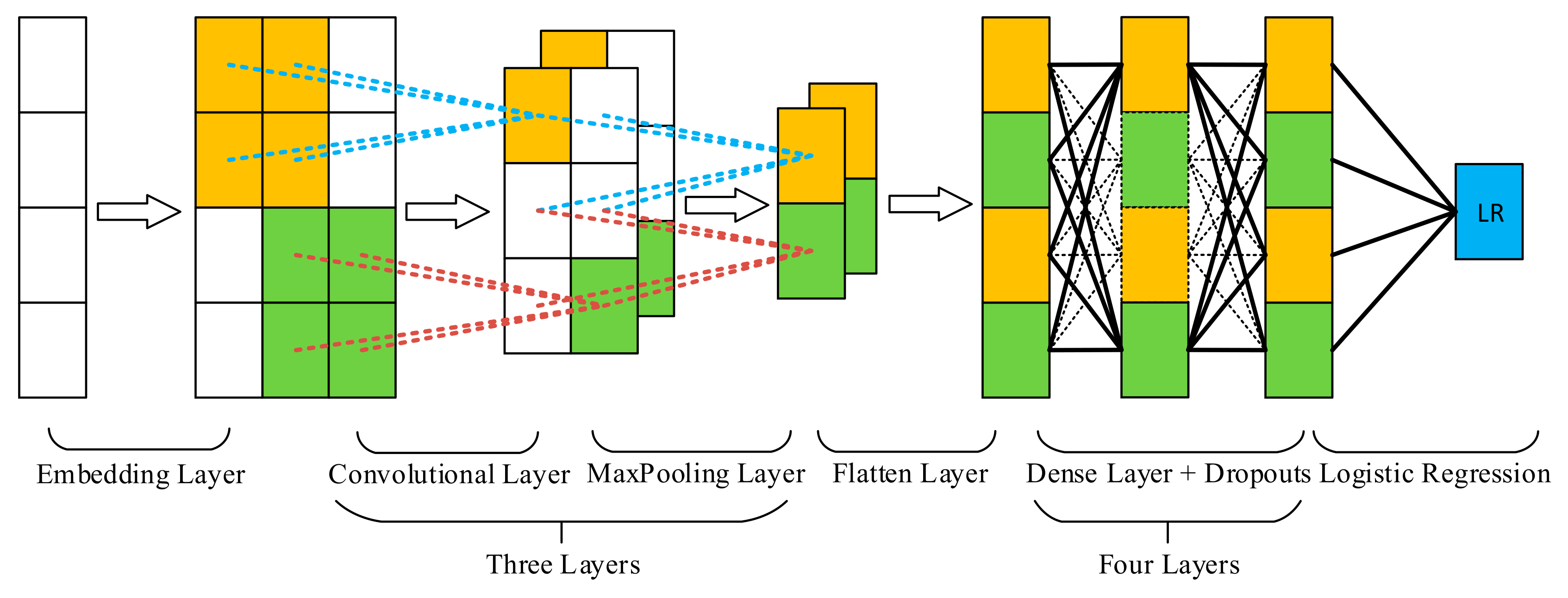
3.4. Building the Improved CNN Model
- Implementation framework: We use Keras (https://www.tensorflow.org/guide/keras), a high-level API based on tensorflow to build our model for simplicity and correctness. The version of tensorflow/keras is 1.8.
- Word embeddings: Note that the implementation of the word embedding layer is also based on Keras; it was wrapped inside the CNN model. Although word embedding is not a part of CNN mathematically, we regarded it as our first layer in our CNN model.
- Three convolutional layers and max-pooling layers: It is universally accepted that increasing the depth of deep models could get better results. Thus, we increased numbers of convolutional layers and max-pooling layers from 1 to 3. Because adding more such layers requires the output of the embedding layer to increase accordingly, which is time-consuming, we did not make further attempts.
- Activation function: Except for the last layer which used the sigmoid activation function for classification, all other layers used the rectified linear unit (ReLU) activation function.
- Parameter initialization: Due to limited calculation resources, large epochs like 100 were not set for training a model. Therefore, it was essential to speed-up model training during the initial epochs. We used He_normal [39] to initialize embedding layers, convolutional layers, and dense layers due to its high efficiency in loss decrease. For the last layer, we used Glorot_normal [40] which targets the sigmoid activation function for initialization.
- Dropouts: We added dropouts between dense layers, which is a common practice to prevent model overfitting [37].
- Regularization: To avoid model overfitting and make the model converge more quickly, we added L2 regularizations for embedding layer and dense layers. When L2 is used, an extra L2 norm of weights is added to the loss function to decrease model capacity, which is essential for model generalization.
- Hyperparameters: We used the best hyperparameter combinations for both experiments on SPSC and PSC dataset, which is illustrate in Section 5.3.
3.5. Predicting Software Defects
4. Experimental Setup
4.1. Evaluation Metrics
4.2. Evaluated Projects and Datasets
4.3. Baseline Methods
- CNN [24]: This is a state-of-the-art method of deep software defect prediction that extracts AST node information as model input, and it proposes deep models (CNN) combined with word embeddings for defect prediction.
- Traditional (LR) [29]: This is an empirical result of traditional software defect prediction, which utilizes 20 code metrics extracted manually in the PROMISE repository as model input, and it proposes logistic regression models for defect prediction. We also used the results from the CNN paper for ease of comparison. It should be noted that the traditional model [29] is not the most suitable baseline to represent traditional machine learning models.
- Five machine learning models [31]: Five models were trained and validated in the within-version WPDP pattern. These five models were the decision tree (DT), logistic regression (LR), naïve Bayes (NB), random torest (RF), and RBF network (NET). These models are the most prevalent machine learning models, which in general represent the top results for WPDP. We excluded the SVM model because it tends to work poorly in empirical scenarios [31].
- RANDOM [31]: This model predicts a source file as buggy at the probability of 0.5. If the RANDOM model beats any model on averaged metrics, it means that the model is worse than random guessing.
- FIX [31]: This model predicts all source files as buggy, which works as a null hypothesis model. If the FIX model beats any model, it means that the model should not be used in practical situations.
4.4. Model Validation Strategy
4.5. Statistical Hypothesis Test
5. Results and Discussion
5.1. Research Questions
- RQ1: Does our improved CNN model outperform state-of-the-art defect prediction methods in WPDP?
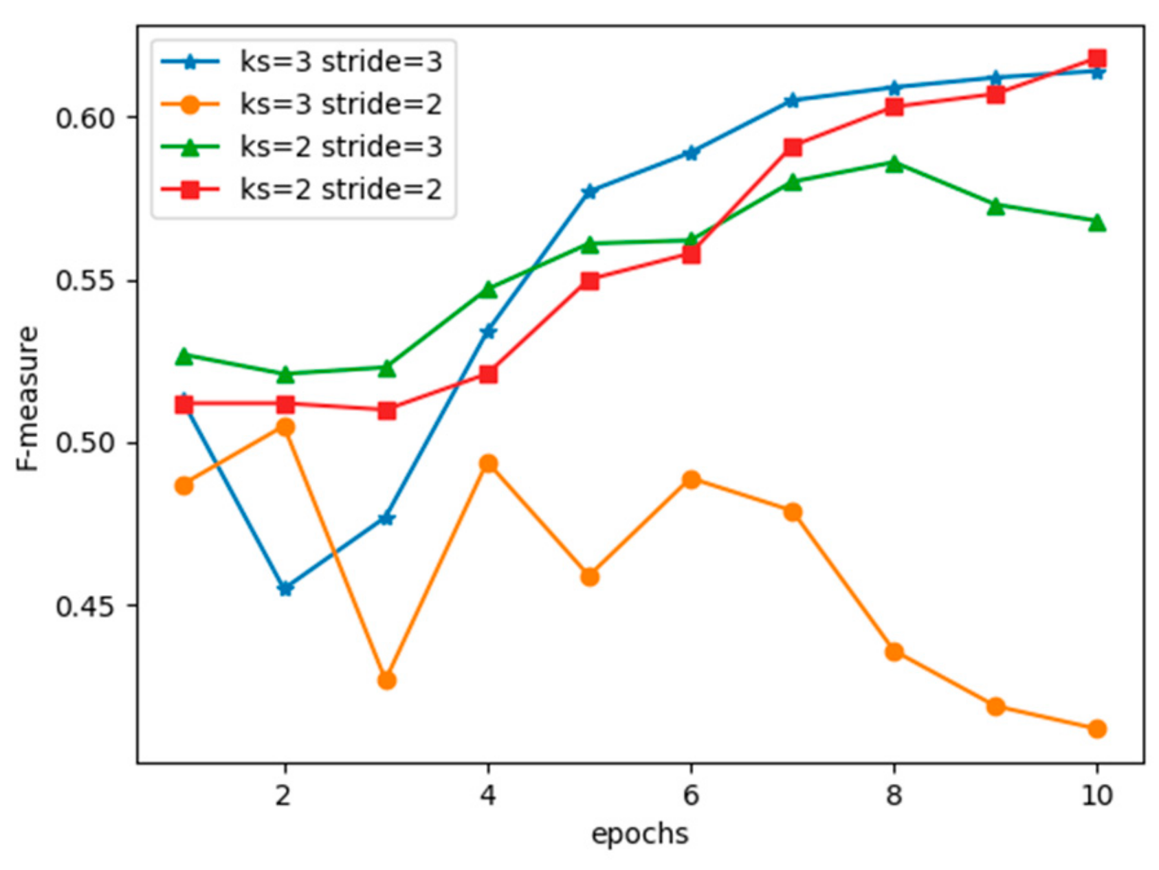
- RQ2: How does the improved CNN model perform under different hyperparameter settings?
- RQ3: Could our model generate results comparable to those of other baseline methods for each version of a project?
5.2. Performance of the Improved CNN Model
5.3. Performance under Different Hyperparameter Settings
5.4. Hyperparameter Instability of Deep Learning Models
6. Threats to Validity
7. Related Works
7.1. Deep Learning Based Software Defect Prediction
7.2. Deep Learning in Software Engineering
8. Conclusions and Future Work
Author Contributions
Funding
Conflicts of Interest
References
- Menzies, T.; Milton, Z.; Turhan, B.; Cukic, B.; Jiang, Y.; Bener, A. Defect prediction from static code features: Current results, limitations, new approaches. Autom. Softw. Eng. 2010, 17, 375–407. [Google Scholar] [CrossRef]
- Moser, R.; Pedrycz, W.; Succi, G. A comparative analysis of the efficiency of change metrics and static code attributes for defect prediction. In Proceedings of the 30th International Conference on Software Engineering, Leipzig, Germany, 15 May 2008; p. 181. [Google Scholar]
- Tan, M.; Tan, L.; Dara, S.; Mayeux, C. Online Defect Prediction for Imbalanced Data. In Proceedings of the 2015 IEEE/ACM 37th IEEE International Conference on Software Engineering (ICSE), Florence, Italy, 16–24 May 2015; pp. 99–108. [Google Scholar]
- Nam, J.; Pan, S.J.; Kim, S. Transfer defect learning. In Proceedings of the International Conference of Software Engineering, San Francisco, CA, USA, 18–26 May 2013. [Google Scholar]
- Nam, J. Survey on Software Defect Prediction. Ph.D. Thesis, The Hong Kong University of Science and Technology, Hong Kong, China, 3 July 2014. [Google Scholar]
- Lyu, M.R. Handbook of Software Reliability Engineering; IEEE Computer Society Press: Washington, DC, USA, 1996; Volume 222. [Google Scholar]
- Halstead, M.H. Elements of Software Science; Elsevier Science Inc.: New York, NY, USA, 1977. [Google Scholar]
- McCabe, T.J. A Complexity Measure. IEEE Trans. Softw. Eng. 1976, SE-2, 308–320. [Google Scholar] [CrossRef]
- Chidamber, S.R.; Kemerer, C.F. A Metrics Suite for Object Oriented Design. IEEE Trans. Softw. Eng. 1994, 20, 476–493. [Google Scholar] [CrossRef]
- Harrison, R.; Counsell, S.; Nithi, R. An evaluation of the MOOD set of object-oriented software metrics. IEEE Trans. Softw. Eng. 1998, 24, 491–496. [Google Scholar] [CrossRef]
- Jiang, T.; Tan, L.; Kim, S. Personalized defect prediction. In Proceedings of the Automated Software Engineering, Silicon Valley, CA, USA, 11–15 November 2013; pp. 279–289. [Google Scholar]
- Gyimothy, T.; Ferenc, R.; Siket, I. Empirical validation of object-oriented metrics on open source software for fault prediction. IEEE Trans. Softw. Eng. 2005, 31, 897–910. [Google Scholar] [CrossRef]
- Zhou, Y.; Leung, H.K.N. Empirical Analysis of Object-Oriented Design Metrics for Predicting High and Low Severity Faults. IEEE Trans. Softw. Eng. 2006, 32, 771–789. [Google Scholar] [CrossRef]
- Lessmann, S.; Baesens, B.; Mues, C.; Pietsch, S. Benchmarking Classification Models for Software Defect Prediction: A Proposed Framework and Novel Findings. IEEE Trans. Softw. Eng. 2008, 34, 485–496. [Google Scholar] [CrossRef]
- Greenwald, J.; Frank, A.; Menzies, T. Data Mining Static Code Attributes to Learn Defect Predictors. IEEE Trans. Softw. Eng. 2007, 33, 2–13. [Google Scholar]
- Jing, X.Y.; Ying, S.; Wu, S.S.; Liu, J. Dictionary learning based software defect prediction. In Proceedings of the 36th International Conference on Software Engineering, Hyderabad, India, 31 May–7 June 2014. [Google Scholar]
- Hindle, A.; Barr, E.T.; Su, Z.; Gabel, M.; Devanbu, P. On the naturalness of software. In Proceedings of the 2012 34th International Conference on Software Engineering (ICSE), Zurich, Switzerland, 2–9 June 2012; pp. 837–847. [Google Scholar]
- Nguyen, A.T.; Nguyen, T.N. Graph-based statistical language model for code. In Proceedings of the 2015 IEEE/ACM 37th IEEE International Conference on Software Engineering, Florence, Italy, 16–24 May 2015; pp. 858–868. [Google Scholar]
- Shippey, T.; Bowes, D.; Hall, T. Automatically identifying code features for software defect prediction: Using AST N-grams. Inf. Softw. Technol. 2018, 106, 142–160. [Google Scholar] [CrossRef]
- White, M.; Vendome, C.; Linares-Vasquez, M.; Poshyvanyk, D. Toward Deep Learning Software Repositories. In Proceedings of the 2015 IEEE/ACM 12th Working Conference on Mining Software Repositories (MSR), Florence, Italy, 16–17 May 2015; pp. 334–345. [Google Scholar]
- Xiao, Y.; Keung, J.; Bennin, K.E.; Mi, Q. Machine translation-based bug localization technique for bridging lexical gap. Inf. Softw. Technol. 2018, 99, 58–61. [Google Scholar] [CrossRef]
- Tu, Z.; Su, Z.; Devanbu, P. On the localness of software. In Proceedings of the 22nd ACM SIGSOFT International Symposium on Foundations of Software Engineering, Hong Kong, China, 16–21 November 2014; pp. 269–280. [Google Scholar]
- Wang, S.; Liu, T.; Tan, L. Automatically learning semantic features for defect prediction. In Proceedings of the 38th International Conference on Software, Austin, TX, USA, 14–22 May 2016; pp. 297–308. [Google Scholar]
- Li, J.; He, P.; Zhu, J.; Lyu, M.R. Software Defect Prediction via Convolutional Neural Network. In Proceedings of the 2017 IEEE International Conference on Software Quality, Reliability and Security (QRS), Prague, Czech Republic, 25–29 July 2017; pp. 318–328. [Google Scholar]
- Krizhevsky, A.; Sutskever, I.; Hinton, G.E. Imagenet classification with deep convolutional neural networks. In Proceedings of the Advances in Neural Information Processing Systems, Lake Tahoe, NV, USA, 3–8 December 2012; pp. 1097–1105. [Google Scholar]
- Goodfellow, I.; Bengio, Y.; Courville, A. Deep learning. Nature 2015, 521, 436–444. [Google Scholar]
- Arcuri, A.; Briand, L. A practical guide for using statistical tests to assess randomized algorithms in software engineering. In Proceedings of the 2011 33rd International Conference on Software Engineering (ICSE), Honolulu, HI, USA, 21–28 May 2011. [Google Scholar]
- Hassan, A.E.; Tantithamthavorn, C.; McIntosh, S.; Matsumoto, K. An Empirical Comparison of Model Validation Techniques for Defect Prediction Models. IEEE Trans. Softw. Eng. 2017, 43, 1–18. [Google Scholar]
- He, Z.; Péters, F.; Menzies, T.; Yang, Y. Learning from Open-Source Projects: An Empirical Study on Defect Prediction. In Proceedings of the 2013 ACM/IEEE International Symposium on Empirical Software Engineering and Measurement (ESEM), Baltimore, MD, USA, 10–11 October 2013; pp. 45–54. [Google Scholar]
- Jureczko, M.; Madeyski, L. Towards identifying software project clusters with regard to defect prediction. In Proceedings of the 6th International Conference on Predictive, Timişoara, Romania, 12–13 September 2010. [Google Scholar]
- Herbold, S.; Trautsch, A.; Grabowski, J. Correction of A Comparative Study to Benchmark Cross-project Defect Prediction Approaches. IEEE Trans. Softw. Eng. 2018, 1. [Google Scholar] [CrossRef]
- Abdel-Hamid, O.; Mohamed, A.-R.; Jiang, H.; Penn, G. Applying Convolutional Neural Networks concepts to hybrid NN-HMM model for speech recognition. In Proceedings of the 2012 IEEE International Conference on Acoustics, Speech and Signal Processing (ICASSP), Kyoto, Japan, 25–30 March 2012; pp. 4277–4280. [Google Scholar]
- LeCun, Y.; Bottou, L.; Bengio, Y.; Haffner, P. Gradient-based learning applied to document recognition. Proc. IEEE 1998, 86, 2278–2324. [Google Scholar] [CrossRef]
- Zhang, X.; Zhao, J.; LeCun, Y. Character-level Convolutional Networks for Text Classification. In Proceedings of the Advances in Neural Information Processing Systems, Montreal, QC, Canada, 7—12 December 2015. [Google Scholar]
- Thom, M.; Palm, G. Sparse activity and sparse connectivity in supervised learning. J. Mach. Learn. Res. 2013, 14, 1091–1143. [Google Scholar]
- Rong, X. word2vec Parameter Learning Explained. Available online: https://arxiv.org/abs/1411.2738 (accessed on 24 January 2019).
- Srivastava, N.; Hinton, G.; Krizhevsky, A.; Sutskever, I.; Salakhutdinov, R. Dropout: A simple way to prevent neural networks from overfitting. J. Mach. Learn. Res. 2014, 15, 1929–1958. [Google Scholar]
- Peng, H.; Mou, L.; Li, G.; Liu, Y.; Zhang, L.; Jin, Z. Building Program Vector Representations for Deep Learning. In Proceedings of the Image Analysis and Processing—ICIAP 2015, Genoa, Italy, 7—11 September 2015; pp. 547–553. [Google Scholar]
- He, K.; Zhang, X.; Ren, S.; Sun, J. Delving Deep into Rectifiers: Surpassing Human-Level Performance on ImageNet Classification. In Proceedings of the 2015 IEEE International Conference on Computer Vision (ICCV), Araucano Park, Chile, 11 December 2015; pp. 1026–1034. [Google Scholar]
- Glorot, X.; Bengio, Y. Understanding the difficulty of training deep feedforward neural networks. In Proceedings of the Thirteenth International Conference on Artificial Intelligence and Statistics, Sardinia, Italy, 13–15 May 2010; pp. 249–256. [Google Scholar]
- Bottou, L. Large-Scale Machine Learning with Stochastic Gradient Descent. In Proceedings of the COMPSTAT’2010; Springer: Berlin, Germany, 2010; pp. 177–186. [Google Scholar]
- Kingma, D.P.; Ba, J. Adam: A Method for Stochastic Optimization. Available online: https://arxiv.org/abs/1412.6980 (accessed on 25 February 2019).
- D’Ambros, M.; Lanza, M.; Robbes, R. An extensive comparison of bug prediction approaches. In Proceedings of the 2010 7th IEEE Working Conference on Mining Software Repositories (MSR 2010), Cape Town, South Africa, 2–3 May 2010. [Google Scholar]
- Zimmermann, T.; Nagappan, N.; Gall, H.; Giger, E.; Murphy, B. Cross-project defect prediction: A large scale experiment on data vs. domain vs. process. In Proceedings of the 7th Joint Meeting of the European Software Engineering Conference and the ACM SIGSOFT Symposium on the Foundations of Software Engineering, Amsterdam, The Netherlands, 24–28 August 2009; pp. 91–100. [Google Scholar]
- Shepperd, M.; Song, Q.; Sun, Z.; Mair, C. Data Quality: Some Comments on the NASA Software Defect Datasets. IEEE Trans. Softw. Eng. 2013, 39, 1208–1215. [Google Scholar] [CrossRef]
- Herzig, K.; Just, S.; Rau, A.; Zeller, A. Predicting defects using change genealogies. In Proceedings of the 2013 IEEE 24th International Symposium on Software Reliability Engineering (ISSRE), Pasadena, CA, USA, 4–7 November 2013; pp. 118–127. [Google Scholar]
- Wu, R.; Zhang, H.; Kim, S.; Cheung, S.C. Relink: Recovering links between bugs and changes. In Proceedings of the 19th ACM SIGSOFT Symposium and the 13th European Conference on Foundations of Software Engineering, Szeged, Hungary, 5–9 September 2011; pp. 15–25. [Google Scholar]
- Friedman, M. The Use of Ranks to Avoid the Assumption of Normality Implicit in the Analysis of Variance. J. Am. Stat. Assoc. 1937, 32, 675–701. [Google Scholar] [CrossRef]
- Holm, S. A simple sequentially rejective multiple test procedure. Scand. J. Stat. 1979, 6, 65–70. [Google Scholar]
- Yang, X.; Lo, D.; Xia, X.; Zhang, Y.; Sun, J. Deep Learning for Just-in-Time Defect Prediction. In Proceedings of the 2015 IEEE International Conference on Software Quality, Reliability and Security (QRS), Vancouver, BC, Canada, 3–5 August 2015; pp. 17–26. [Google Scholar]
- Tong, H.; Liu, B.; Wang, S. Software defect prediction using stacked denoising autoencoders and two-stage ensemble learning. Inf. Softw. Technol. 2018, 96, 94–111. [Google Scholar] [CrossRef]
- Zhang, X. Using Cross-Entropy Value of Code for Better Defect Prediction. Int. J. Perform. Eng. 2018, 14, 2105. [Google Scholar] [CrossRef][Green Version]
- Dam, H.K.; Pham, T.; Ng, S.W.; Tran, T.; Grundy, J.; Ghose, A.; Kim, C.J. A Deep Tree-Based Model for Software Defect Prediction. Available online: https://arxiv.org/abs/1802.00921 (accessed on 24 January 2019).
- Phan, A.V.; Nguyen, L.M.; Bui, L.T. Convolutional neural networks over control flow graphs for software defect prediction. In Proceedings of the 2017 IEEE 29th International Conference on Tools with Artificial Intelligence (ICTAI), Boston, MA, USA, 6–8 November 2017; pp. 45–52. [Google Scholar]
- Phan, A.V.; Nguyen, L.M. Convolutional neural networks on assembly code for predicting software defects. In Proceedings of the 2017 21st Asia Pacific Symposium on Intelligent and Evolutionary Systems (IES), Hanoi, Vietnam, 15–17 November 2017. [Google Scholar]
- Cheng, J.; Guo, J.; Cleland-Huang, J. Semantically Enhanced Software Traceability Using Deep Learning Techniques. In Proceedings of the 2017 IEEE/ACM 39th International Conference on Software Engineering (ICSE), Buenos Aires, Argentina, 20–28 May 2017; pp. 3–14. [Google Scholar]
- Li, L.; Feng, H.; Zhuang, W.; Meng, N.; Ryder, B. CCLearner: A Deep Learning-Based Clone Detection Approach. In Proceedings of the IEEE International Conference on Software Maintenance and Evolution (ICSME), Shangai, China, 17–24 September 2017; pp. 249–260. [Google Scholar]
- Lam, A.N.; Nguyen, A.T.; Nguyen, H.A.; Nguyen, T.N. Bug localization with combination of deep learning and information retrieval. In Proceedings of the 2017 IEEE/ACM 25th International Conference on Program Comprehension (ICPC), Buenos Aires, Argentina, 22–23 May 2017; pp. 218–229. [Google Scholar]
- Pradel, M.; Sen, K. DeepBugs: A learning approach to name-based bug detection. Proc. ACM Program. Lang. 2018, 2, 1–25. [Google Scholar] [CrossRef]
- Reyes, J.; Ramirez, D.; Paciello, J. Automatic Classification of Source Code Archives by Programming Language: A Deep Learning Approach. In Proceedings of the International Conference on Computational Science and Computational Intelligence (CSCI), Las Vegas, NV, USA, 15–17 December 2016; 2016; pp. 514–519. [Google Scholar]
- Zekany, S.; Rings, D.; Harada, N.; Laurenzano, M.A.; Tang, L.; Mars, J. CrystalBall: Statically analyzing runtime behavior via deep sequence learning. In Proceedings of the 2016 49th Annual IEEE/ACM International Symposium on Microarchitecture (MICRO), Taipei, Taiwan, 15–19 October 2016; pp. 1–12. [Google Scholar]
- Corley, C.S.; Damevski, K.; Kraft, N.A. Exploring the use of deep learning for feature location. In Proceedings of the 2015 IEEE International Conference on Software Maintenance and Evolution (ICSME), Bremen, Germany, 29 September–1 October 2015; pp. 556–560. [Google Scholar]
- Pang, Y.; Xue, X.; Wang, H. Predicting Vulnerable Software Components through Deep Neural Network. In Proceedings of the 2017 International Conference on Deep Learning Technologies, Chengdu China, 2–4 June 2017; pp. 6–10. [Google Scholar]
- Bandara, U.; Wijayarathna, G. Deep Neural Networks for Source Code Author Identification. In Proceedings of the 20th International Conference, Daegu, Korea, 3–7 November 2013; pp. 368–375. [Google Scholar]


| Li’s CNN | Improved CNN | |
|---|---|---|
| Embedding layer | Yes | Yes |
| #Convolutional Layers | 1 | 3 |
| #Pooling layers | 1 | 3 |
| Activation function | ReLU + sigmoid (last dense layer) | ReLU + sigmoid (last dense layer) |
| Parameter initialization | None | He_normal (embedding layer, convolutional layer, dense layers) Glorot_normal (last dense layer) |
| Dropouts | None | Between dense layers |
| Regularization | None | L2 Regularization (embedding layer, dense layers) |
| Training and optimizer | Mini-batch SGD + Adam (loss function not given) | Mini-batch SGD + Adam + binary cross-entropy |
| Project | Versions (Vp, Vn) | #Files | #Defects | Avg. Buggy Rate (%) |
|---|---|---|---|---|
| Camel | 1.4, 1.6 | 1781(–6) | 333(0) | 18.7(+0.6) |
| jEdit | 4.0, 4.1 | 547(–71) | 134(–20) | 24.5(–0.4) |
| Lucene | 2.0, 2.2 | 420(–22) | 234(–1) | 55.7(+2.5) |
| Xalan | 2.5, 2.6 | 1629(–59) | 790(–8) | 48.5(+1.2) |
| Xerces | 1.2, 1.3 | 882(–11) | 138(–2) | 15.6(–0.1) |
| Synapse | 1.1, 1.2 | 461(–17) | 141(–5) | 30.6(+0.1) |
| Poi | 2.5, 3.0 | 818(–9) | 529(–9) | 64.7(+0.7) |
| Total | - | 6538(–245) | 2299(–45) | 35.2(+0.6) |
| Project | Version | #Files | #Defects | Buggy Rate (%) |
|---|---|---|---|---|
| Ant | 1.3 | 124(–) | 20(0) | 16.0(+0.1) |
| 1.4 | 177(–1) | 40(0) | 22.6(+0.1) | |
| 1.5 | 278(–15) | 29(–3) | 10.4(–0.5) | |
| 1.6 | 350(–1) | 92(0) | 26.3(+0.1) | |
| 1.7 | 741(–4) | 166(–1) | 22.4(0) | |
| Camel | 1.0 | 339(–0) | 13(0) | 3.8(0) |
| 1.2 | 595(–13) | 216(0) | 36.3(+0.8) | |
| 1.4 | 847(–25) | 145(0) | 17.1(+0.5) | |
| 1.6 | 934(–31) | 188(0) | 20.1(+0.6) | |
| Ivy | 1.1 | 111(0) | 63(0) | 56.8(0) |
| 1.4 | 241(0) | 16(0) | 6.6(0) | |
| 2.0 | 352(0) | 40(0) | 11.4(0) | |
| JEdit | 3.2 | 260(–12) | 90(0) | 34.6(+1.5) |
| 4.0 | 281(–25) | 67(–8) | 23.8(–0.7) | |
| 4.1 | 266(–46) | 67(–12) | 25.2(–0.1) | |
| 4.2 | 355(–12) | 48(0) | 13.5(+0.4) | |
| 4.3 | 487(–5) | 11(0) | 2.3(0) | |
| Log4j | 1.0 | 119(–16) | 34(0) | 28.8(+3.4) |
| 1.1 | 104(–5) | 37(0) | 35.6(+1.6) | |
| 1.2 | 194(–11) | 186(–3) | 95.9(+3.7) | |
| Lucene | 2.0 | 186(–9) | 91(0) | 48.9(+2.3) |
| 2.2 | 234(–13) | 143(–1) | 61.1(+2.8) | |
| 2.4 | 330(–10) | 203(0) | 61.5(+1.8) | |
| Pbeans | 1.0 | 26(0) | 20(0) | 76.9(0) |
| 2.0 | 51(0) | 10(0) | 19.6(0) | |
| Poi | 1.5 | 235(–2) | 141(0) | 60.0(+0.5) |
| 2.0 | 309(–5) | 37(0) | 12.0(+0.2) | |
| 2.5 | 380(–5) | 248(0) | 65.3(+0.8) | |
| 3.0 | 438(–4) | 529(0) | 64.2(+0.6) | |
| Synapse | 1.0 | 157(0) | 16(0) | 10.2(0) |
| 1.1 | 205(–17) | 55(–5) | 26.8(–0.2) | |
| 1.2 | 256(0) | 86(0) | 33.6(0) | |
| Velocity | 1.4 | 195(–1) | 147(0) | 75.4(+0.4) |
| 1.5 | 214(0) | 142(0) | 66.4(0) | |
| 1.6 | 229(0) | 78(0) | 34.1(0) | |
| Xalan | 2.4 | 676(–47) | 110(0) | 16.3(+1.1) |
| 2.5 | 754(–49) | 379(–8) | 50.3(+2.1) | |
| 2.6 | 875(–10) | 411(0) | 47.0(+0.5) | |
| Xerces | Initial | 162(0) | 77(0) | 47.5(0) |
| 1.2 | 436(–4) | 70(–1) | 16.1(–0.1) | |
| 1.3 | 446(–7) | 68(–1) | 15.2(0) | |
| Total | - | 14,066(–289) | 6542(–77) | 31.4(+0.6) |
| Project | Traditional (LR) | DBN | Li’s CNN | Improved CNN |
|---|---|---|---|---|
| Camel | 0.329 | 0.335 | 0.505 | 0.487 |
| JEdit | 0.573 | 0.480 | 0.631 | 0.590 |
| Lucene | 0.618 | 0.758 | 0.761 | 0.701 |
| Xalan | 0.627 | 0.681 | 0.676 | 0.780 |
| Xerces | 0.273 | 0.261 | 0.311 | 0.667 |
| Synapse | 0.500 | 0.503 | 0.512 | 0.655 |
| Poi | 0.748 | 0.780 | 0.778 | 0.444 |
| average | 0.524 | 0.543 | 0.596 | 0.618 |
| Traditional (LR) | DBN | Li’s CNN | |
|---|---|---|---|
| DBN | 0.1098 | - | - |
| Li’s CNN | 0.0038 | 0.0790 | - |
| Improved CNN | 0.0079 | 0.1563 | 0.5339 |
| Project. | Version | DT | RF | LR | NB | NET | FIX | RANDOM | Improved CNN |
|---|---|---|---|---|---|---|---|---|---|
| Ant | 1.3 | 0.36 | 0.31 | 0.36 | 0.43 | 0.14 | 0.28 | 0.24 | 0.67 |
| 1.4 | 0.40 | 0.24 | 0.22 | 0.44 | 0.04 | 0.37 | 0.32 | 0.38 | |
| 1.5 | 0.42 | 0.37 | 0.41 | 0.35 | 0.15 | 0.20 | 0.18 | 0.25 | |
| 1.6 | 0.55 | 0.59 | 0.57 | 0.58 | 0.59 | 0.42 | 0.33 | 0.41 | |
| 1.7 | 0.53 | 0.52 | 0.50 | 0.56 | 0.45 | 0.36 | 0.31 | 0.39 | |
| Camel | 1.0 | 0.00 | 0.00 | 0.00 | 0.30 | 0.00 | 0.07 | 0.08 | 0.40 |
| 1.2 | 0.46 | 0.40 | 0.35 | 0.32 | 0.26 | 0.52 | 0.41 | 0.69 | |
| 1.4 | 0.30 | 0.27 | 0.18 | 0.26 | 0.05 | 0.29 | 0.25 | 0.46 | |
| 1.6 | 0.27 | 0.25 | 0.18 | 0.30 | 0.16 | 0.33 | 0.28 | 0.52 | |
| Ivy | 1.1 | 0.73 | 0.71 | 0.71 | 0.54 | 0.73 | 0.72 | 0.55 | 0.80 |
| 1.4 | 0.00 | 0.00 | 0.15 | 0.17 | 0.11 | 0.12 | 0.11 | 0.22 | |
| 2.0 | 0.17 | 0.31 | 0.31 | 0.40 | 0.16 | 0.20 | 0.18 | 0.31 | |
| JEdit | 3.2 | 0.56 | 0.63 | 0.68 | 0.55 | 0.59 | 0.50 | 0.40 | 0.69 |
| 4.0 | 0.49 | 0.56 | 0.49 | 0.41 | 0.43 | 0.39 | 0.31 | 0.48 | |
| 4.1 | 0.45 | 0.54 | 0.61 | 0.52 | 0.54 | 0.40 | 0.33 | 0.41 | |
| 4.2 | 0.46 | 0.29 | 0.37 | 0.44 | 0.38 | 0.23 | 0.20 | 0.58 | |
| 4.3 | 0.00 | 0.00 | 0.00 | 0.21 | 0.00 | 0.04 | 0.04 | 0.00 | |
| Log4j | 1.0 | 0.55 | 0.53 | 0.55 | 0.61 | 0.59 | 0.40 | 0.36 | 0.77 |
| 1.1 | 0.66 | 0.73 | 0.63 | 0.72 | 0.76 | 0.51 | 0.43 | 0.40 | |
| 1.2 | 0.95 | 0.96 | 0.94 | 0.67 | 0.96 | 0.96 | 0.63 | 0.97 | |
| Lucene | 2.0 | 0.58 | 0.59 | 0.65 | 0.54 | 0.66 | 0.64 | 0.48 | 0.74 |
| 2.2 | 0.62 | 0.67 | 0.70 | 0.48 | 0.66 | 0.74 | 0.53 | 0.63 | |
| 2.4 | 0.72 | 0.73 | 0.74 | 0.54 | 0.71 | 0.75 | 0.54 | 0.77 | |
| Pbeans | 1.0 | 0.87 | 0.90 | 0.79 | 0.81 | 0.81 | 0.87 | 0.66 | 0.89 |
| 2.0 | 0.22 | 0.35 | 0.48 | 0.25 | 0.14 | 0.33 | 0.30 | 0.67 | |
| Poi | 1.5 | 0.79 | 0.75 | 0.73 | 0.46 | 0.77 | 0.75 | 0.55 | 0.61 |
| 2.0 | 0.26 | 0.25 | 0.23 | 0.27 | 0.14 | 0.21 | 0.20 | 0.13 | |
| 2.5 | 0.82 | 0.85 | 0.82 | 0.56 | 0.82 | 0.78 | 0.58 | 0.90 | |
| 3.0 | 0.83 | 0.84 | 0.81 | 0.49 | 0.82 | 0.78 | 0.56 | 0.76 | |
| Synapse | 1.0 | 0.08 | 0.09 | 0.32 | 0.41 | 0.19 | 0.18 | 0.16 | 0.29 |
| 1.1 | 0.53 | 0.51 | 0.58 | 0.56 | 0.52 | 0.43 | 0.35 | 0.67 | |
| 1.2 | 0.60 | 0.59 | 0.55 | 0.59 | 0.56 | 0.50 | 0.39 | 0.69 | |
| Velocity | 1.4 | 0.90 | 0.89 | 0.89 | 0.89 | 0.91 | 0.86 | 0.60 | 0.90 |
| 1.5 | 0.80 | 0.83 | 0.80 | 0.45 | 0.78 | 0.80 | 0.57 | 0.78 | |
| 1.6 | 0.54 | 0.50 | 0.51 | 0.38 | 0.47 | 0.51 | 0.41 | 0.83 | |
| Xalan | 2.4 | 0.26 | 0.28 | 0.28 | 0.37 | 0.16 | 0.26 | 0.23 | 0.25 |
| 2.5 | 0.67 | 0.65 | 0.58 | 0.38 | 0.48 | 0.65 | 0.49 | 0.70 | |
| 2.6 | 0.72 | 0.73 | 0.69 | 0.61 | 0.62 | 0.63 | 0.47 | 0.76 | |
| Xerces | Initial | 0.71 | 0.68 | 0.73 | 0.34 | 0.63 | 0.64 | 0.48 | 0.65 |
| 1.2 | 0.38 | 0.33 | 0.07 | 0.23 | 0.03 | 0.28 | 0.24 | 0.41 | |
| 1.3 | 0.50 | 0.44 | 0.42 | 0.38 | 0.35 | 0.26 | 0.22 | 0.56 | |
| average | 0.51 | 0.50 | 0.50 | 0.46 | 0.45 | 0.47 | 0.36 | 0.57 | |
| Project | Version | DT | RF | LR | NB | NET | FIX | RANDOM | Improved CNN |
|---|---|---|---|---|---|---|---|---|---|
| Ant | 1.3 | 0.50 | 0.39 | 0.50 | 0.63 | 0.18 | 0.00 | 0.49 | 0.67 |
| 1.4 | 0.56 | 0.29 | 0.29 | 0.58 | 0.05 | 0.00 | 0.51 | 0.51 | |
| 1.5 | 0.51 | 0.44 | 0.47 | 0.69 | 0.17 | 0.00 | 0.50 | 0.28 | |
| 1.6 | 0.66 | 0.66 | 0.64 | 0.67 | 0.69 | 0.00 | 0.48 | 0.53 | |
| 1.7 | 0.65 | 0.60 | 0.55 | 0.68 | 0.50 | 0.00 | 0.51 | 0.46 | |
| Camel | 1.0 | 0.00 | 0.00 | 0.00 | 0.62 | 0.00 | 0.00 | 0.54 | 0.50 |
| 1.2 | 0.54 | 0.46 | 0.41 | 0.36 | 0.28 | 0.00 | 0.49 | 0.76 | |
| 1.4 | 0.37 | 0.30 | 0.20 | 0.35 | 0.05 | 0.00 | 0.49 | 0.54 | |
| 1.6 | 0.35 | 0.29 | 0.19 | 0.37 | 0.17 | 0.00 | 0.50 | 0.60 | |
| Ivy | 1.1 | 0.62 | 0.67 | 0.67 | 0.55 | 0.69 | 0.00 | 0.51 | 0.65 |
| 1.4 | 0.00 | 0.00 | 0.22 | 0.31 | 0.12 | 0.00 | 0.48 | 0.49 | |
| 2.0 | 0.18 | 0.37 | 0.37 | 0.60 | 0.18 | 0.00 | 0.49 | 0.40 | |
| JEdit | 3.2 | 0.65 | 0.69 | 0.74 | 0.61 | 0.64 | 0.00 | 0.50 | 0.73 |
| 4.0 | 0.59 | 0.63 | 0.56 | 0.49 | 0.48 | 0.00 | 0.48 | 0.65 | |
| 4.1 | 0.55 | 0.60 | 0.68 | 0.59 | 0.58 | 0.00 | 0.49 | 0.00 | |
| 4.2 | 0.60 | 0.34 | 0.42 | 0.58 | 0.42 | 0.00 | 0.49 | 0.78 | |
| 4.3 | 0.00 | 0.00 | 0.00 | 0.53 | 0.00 | 0.00 | 0.49 | 0.00 | |
| Log4j | 1.0 | 0.66 | 0.60 | 0.64 | 0.66 | 0.65 | 0.00 | 0.52 | 0.81 |
| 1.1 | 0.72 | 0.76 | 0.70 | 0.77 | 0.79 | 0.00 | 0.52 | 0.44 | |
| 1.2 | 0.40 | 0.31 | 0.12 | 0.63 | 0.00 | 0.00 | 0.45 | 0.00 | |
| Lucene | 2.0 | 0.62 | 0.63 | 0.68 | 0.58 | 0.69 | 0.00 | 0.51 | 0.75 |
| 2.2 | 0.53 | 0.62 | 0.56 | 0.49 | 0.52 | 0.00 | 0.49 | 0.62 | |
| 2.4 | 0.67 | 0.67 | 0.69 | 0.55 | 0.65 | 0.00 | 0.49 | 0.00 | |
| Pbeans | 1.0 | 0.75 | 0.77 | 0.60 | 0.71 | 0.28 | 0.00 | 0.53 | 0.89 |
| 2.0 | 0.32 | 0.45 | 0.68 | 0.33 | 0.18 | 0.00 | 0.50 | 0.67 | |
| Poi | 1.5 | 0.74 | 0.69 | 0.61 | 0.47 | 0.61 | 0.00 | 0.50 | 0.61 |
| 2.0 | 0.32 | 0.32 | 0.28 | 0.39 | 0.15 | 0.00 | 0.51 | 0.25 | |
| 2.5 | 0.76 | 0.81 | 0.72 | 0.56 | 0.71 | 0.00 | 0.52 | 0.82 | |
| 3.0 | 0.75 | 0.78 | 0.73 | 0.49 | 0.72 | 0.00 | 0.50 | 0.72 | |
| Synapse | 1.0 | 0.12 | 0.12 | 0.47 | 0.74 | 0.22 | 0.00 | 0.47 | 0.49 |
| 1.1 | 0.63 | 0.57 | 0.66 | 0.68 | 0.56 | 0.00 | 0.49 | 0.70 | |
| 1.2 | 0.67 | 0.65 | 0.62 | 0.66 | 0.62 | 0.00 | 0.49 | 0.72 | |
| Velocity | 1.4 | 0.71 | 0.72 | 0.70 | 0.70 | 0.67 | 0.00 | 0.50 | 0.66 |
| 1.5 | 0.60 | 0.73 | 0.65 | 0.46 | 0.57 | 0.00 | 0.51 | 0.72 | |
| 1.6 | 0.62 | 0.58 | 0.58 | 0.42 | 0.51 | 0.00 | 0.51 | 0.84 | |
| Xalan | 2.4 | 0.34 | 0.33 | 0.32 | 0.51 | 0.18 | 0.00 | 0.50 | 0.31 |
| 2.5 | 0.66 | 0.67 | 0.61 | 0.41 | 0.53 | 0.00 | 0.50 | 0.69 | |
| 2.6 | 0.74 | 0.75 | 0.71 | 0.62 | 0.65 | 0.00 | 0.49 | 0.78 | |
| Xerces | Initial | 0.73 | 0.70 | 0.49 | 0.36 | 0.41 | 0.00 | 0.49 | 0.58 |
| 1.2 | 0.49 | 0.38 | 0.73 | 0.32 | 0.65 | 0.00 | 0.49 | 0.66 | |
| 1.3 | 0.60 | 0.51 | 0.08 | 0.50 | 0.03 | 0.00 | 0.48 | 0.65 | |
| average | 0.52 | 0.51 | 0.50 | 0.54 | 0.41 | 0.00 | 0.50 | 0.56 | |
| Project | Version | DT | RF | LR | NB | NET | FIX | RANDOM | Improved CNN |
|---|---|---|---|---|---|---|---|---|---|
| Ant | 1.3 | 0.24 | 0.23 | 0.24 | 0.30 | 0.05 | 0.00 | 0.00 | 0.68 |
| 1.4 | 0.22 | 0.12 | 0.06 | 0.23 | −0.04 | 0.00 | 0.02 | 0.20 | |
| 1.5 | 0.38 | 0.33 | 0.38 | 0.27 | 0.14 | 0.00 | 0.00 | 0.24 | |
| 1.6 | 0.40 | 0.49 | 0.45 | 0.45 | 0.46 | 0.00 | 0.03 | 0.22 | |
| 1.7 | 0.40 | 0.43 | 0.42 | 0.44 | 0.39 | 0.00 | 0.01 | 0.30 | |
| Camel | 1.0 | 0.00 | −0.02 | −0.02 | 0.28 | −0.01 | 0.00 | 0.03 | 0.39 |
| 1.2 | 0.21 | 0.19 | 0.18 | 0.14 | 0.19 | 0.00 | 0.01 | 0.50 | |
| 1.4 | 0.21 | 0.23 | 0.16 | 0.14 | 0.06 | 0.00 | 0.01 | 0.39 | |
| 1.6 | 0.16 | 0.19 | 0.16 | 0.21 | 0.18 | 0.00 | 0.01 | 0.42 | |
| Ivy | 1.1 | 0.31 | 0.34 | 0.34 | 0.26 | 0.38 | 0.00 | 0.04 | 0.48 |
| 1.4 | −0.02 | 0.00 | 0.11 | 0.11 | 0.16 | 0.00 | 0.01 | 0.16 | |
| 2.0 | 0.23 | 0.27 | 0.27 | 0.31 | 0.17 | 0.00 | 0.01 | 0.25 | |
| JEdit | 3.2 | 0.37 | 0.48 | 0.53 | 0.40 | 0.46 | 0.00 | 0.00 | 0.56 |
| 4.0 | 0.34 | 0.45 | 0.39 | 0.29 | 0.36 | 0.00 | 0.03 | 0.29 | |
| 4.1 | 0.30 | 0.45 | 0.50 | 0.40 | 0.46 | 0.00 | 0.02 | 0.00 | |
| 4.2 | 0.39 | 0.26 | 0.33 | 0.36 | 0.37 | 0.00 | 0.01 | 0.51 | |
| 4.3 | 0.00 | −0.01 | −0.02 | 0.20 | 0.00 | 0.00 | 0.00 | 0.00 | |
| Log4j | 1.0 | 0.40 | 0.42 | 0.42 | 0.53 | 0.49 | 0.00 | 0.04 | 0.69 |
| 1.1 | 0.50 | 0.62 | 0.46 | 0.60 | 0.66 | 0.00 | 0.04 | 0.29 | |
| 1.2 | 0.27 | 0.27 | 0.04 | 0.17 | −0.02 | 0.00 | 0.04 | 0.00 | |
| Lucene | 2.0 | 0.24 | 0.30 | 0.38 | 0.32 | 0.40 | 0.00 | 0.02 | 0.53 |
| 2.2 | 0.07 | 0.23 | 0.21 | 0.19 | 0.12 | 0.00 | 0.01 | 0.29 | |
| 2.4 | 0.34 | 0.34 | 0.37 | 0.33 | 0.30 | 0.00 | 0.01 | 0.00 | |
| Pbeans | 1.0 | 0.49 | 0.57 | 0.23 | 0.37 | 0.02 | 0.00 | 0.09 | 0.63 |
| 2.0 | 0.06 | 0.23 | 0.33 | 0.13 | 0.04 | 0.00 | 0.05 | 0.67 | |
| Poi | 1.5 | 0.48 | 0.39 | 0.28 | 0.24 | 0.35 | 0.00 | 0.00 | 0.29 |
| 2.0 | 0.22 | 0.19 | 0.18 | 0.19 | 0.15 | 0.00 | 0.01 | 0.01 | |
| 2.5 | 0.52 | 0.60 | 0.47 | 0.28 | 0.46 | 0.00 | 0.03 | 0.70 | |
| 3.0 | 0.52 | 0.56 | 0.49 | 0.26 | 0.48 | 0.00 | 0.00 | 0.42 | |
| Synapse | 1.0 | 0.01 | 0.04 | 0.25 | 0.35 | 0.18 | 0.00 | 0.03 | 0.20 |
| 1.1 | 0.36 | 0.39 | 0.46 | 0.38 | 0.43 | 0.00 | 0.01 | 0.60 | |
| 1.2 | 0.41 | 0.44 | 0.39 | 0.42 | 0.41 | 0.00 | 0.01 | 0.59 | |
| Velocity | 1.4 | 0.56 | 0.52 | 0.51 | 0.53 | 0.59 | 0.00 | 0.01 | 0.56 |
| 1.5 | 0.33 | 0.49 | 0.38 | 0.19 | 0.27 | 0.00 | 0.02 | 0.42 | |
| 1.6 | 0.34 | 0.31 | 0.32 | 0.24 | 0.33 | 0.00 | 0.02 | 0.76 | |
| Xalan | 2.4 | 0.17 | 0.23 | 0.26 | 0.27 | 0.16 | 0.00 | 0.00 | 0.18 |
| 2.5 | 0.32 | 0.37 | 0.25 | 0.13 | 0.16 | 0.00 | 0.01 | 0.38 | |
| 2.6 | 0.48 | 0.53 | 0.47 | 0.45 | 0.40 | 0.00 | 0.01 | 0.58 | |
| Xerces | Initial | 0.47 | 0.42 | 0.46 | 0.19 | 0.32 | 0.00 | 0.01 | 0.23 |
| 1.2 | 0.29 | 0.28 | 0.04 | 0.12 | 0.11 | 0.00 | 0.01 | 0.28 | |
| 1.3 | 0.43 | 0.40 | 0.37 | 0.29 | 0.31 | 0.00 | 0.02 | 0.50 | |
| average | 0.30 | 0.33 | 0.30 | 0.29 | 0.27 | 0.00 | 0.02 | 0.38 | |
| DT | RF | LR | NB | NET | |
|---|---|---|---|---|---|
| RF | 1 | - | - | - | - |
| LR | 0.0857 | 0.0857 | - | - | - |
| NB | 0 | 0 | 0.0752 | - | - |
| NET | 0 | 0 | 0 | 0.0605 | - |
| Improved CNN | 0 | 0 | 0 | 0 | 0 |
| DT | RF | LR | NB | NET | |
|---|---|---|---|---|---|
| RF | 1 | - | - | - | - |
| LR | 0.0231 | 0.0869 | - | - | - |
| NB | 0.0559 | 0.1766 | 1 | - | - |
| NET | 0 | 0 | 0 | 0 | - |
| Improved CNN | 0.0231 | 0.0028 | 0 | 0 | 0 |
| DT | RF | LR | NB | NET | |
|---|---|---|---|---|---|
| RF | 0.0069 | - | - | - | - |
| LR | 0.5251 | 0.0009 | - | - | - |
| NB | 0.2749 | 0 | 0.4681 | - | - |
| NET | 0.0026 | 0 | 0.0169 | 0.2749 | - |
| Improved CNN | 0 | 0.1102 | 0 | 0 | 0 |
© 2019 by the authors. Licensee MDPI, Basel, Switzerland. This article is an open access article distributed under the terms and conditions of the Creative Commons Attribution (CC BY) license (http://creativecommons.org/licenses/by/4.0/).
Share and Cite
Pan, C.; Lu, M.; Xu, B.; Gao, H. An Improved CNN Model for Within-Project Software Defect Prediction. Appl. Sci. 2019, 9, 2138. https://doi.org/10.3390/app9102138
Pan C, Lu M, Xu B, Gao H. An Improved CNN Model for Within-Project Software Defect Prediction. Applied Sciences. 2019; 9(10):2138. https://doi.org/10.3390/app9102138
Chicago/Turabian StylePan, Cong, Minyan Lu, Biao Xu, and Houleng Gao. 2019. "An Improved CNN Model for Within-Project Software Defect Prediction" Applied Sciences 9, no. 10: 2138. https://doi.org/10.3390/app9102138
APA StylePan, C., Lu, M., Xu, B., & Gao, H. (2019). An Improved CNN Model for Within-Project Software Defect Prediction. Applied Sciences, 9(10), 2138. https://doi.org/10.3390/app9102138