Coordinated Dispatch of Integrated Energy Systems Considering the Differences of Multiple Functional Areas

Abstract

A large amount of wind turbine power and photovoltaic power is abandoned in many areas with abundant renewable energy due to thermal-electric coupling, inadequate local consumption capacity, and limited capacity of transmission lines, etc. To solve the above problems, a coordinated dispatching method for integrated energy systems is proposed in this paper. Firstly, the spatiotemporal characteristics of diversified loads in multiple functional areas are introduced, including the inertia and elasticity of heating/cooling loads, the spatiotemporal distribution of electric vehicles, and the optimum transmission distance of diversified loads, etc. Secondly, a coordinated dispatching model of integrated energy systems is proposed, which considers the differences of multiple functional areas and various forms of energy systems. Finally, an actual distribution system in Jianshan District, Haining, Zhejiang Province of China is investigated for demonstrating the effectiveness of the proposed model. The results illustrate that the proposed model could effectively improve the consumption rate of renewable energy and reduce the volatility of renewable energy by considering the coordination of electric vehicles, tie lines, and heating/cooling systems in multiple functional areas.

1. Introduction

With the increasing proportion of renewable energy in the whole energy supply, its consumption has increasingly become one of key problems to be solved, and the abandonment of wind turbine (WT) power and photovoltaic (PV) power has not been solved [1]. According to the statistics of the National Energy Administration of China, the annual abandonment of WT power in China reached 41.9 billion kWh in 2017 [2]. The abandonment rate of WT power in some areas of China has exceeded 40%. The western region is an important area for the development of PV power in China and its installed PV capacity is still growing rapidly, but the average abandonment rate of PV power in China has reached 20%.

The reasons for the abandonment of WT and PV powers are different from place to place, mainly due to the factors such as thermal-electric coupling, inadequate local consumption capacity, and limitation of transmission line capacity [3,4]. Taking Jianshan District, Haining, Zhejiang Province of China as an example, in 2018, the total installed capacity of WT and PV power in this region was 230 MW, and its load level was only around 150 MW, which is a typical area with abundant renewable energy. Under normal circumstances, the area basically achieves self-balancing of electric power. But under special circumstances, the loads of the industrial area during the holidays, for example, are drastically reduced, and it is impossible to achieve self-balancing of electric power. The excess energy could only be transferred back to the 220 kV Anjiang Substation through the 110 kV Jianshan Substation, or even be transferred to the transmission system through the 220 kV Anjiang Substation. However, due to the capacity limitation of the main transformer in the Jianshan Substation, the Jianshan distribution systems cannot fully meet the needs of the delivery of the excess renewable energy. The limited capacity of WT and PV has reached 97 MW, and the limited proportion has reached 42.17%.

The integrated energy system (IES) coordinates the various forms of energy systems such as the distribution systems, the renewable energy systems, and the traffic systems considering electric vehicles (EVs) and the combined cooling, heating, and power (CCHP) systems, which could realize the optimal utilization of various types of energy and effectively solve the consumption problem of renewable energy [5]. In [6], the optimization of the IES including district heating, cooling, and various forms of energy storage in Singapore was performed, and the results show that the cost of energy through methane storage or heat storage is much less than that of using electricity storage or hydrogen storage when the space constraints of photovoltaic installations are taken into consideration. In [7,8], the consumption rate of WT in the CCHP systems is improved through energy storage, the output of the CCHP units is reduced when the WT surges, and the energy storage device is utilized to meet the user’s cooling and heating demand for reducing the abandoned power of WT.

Generally, the installation costs of energy storage devices are relatively high and energy storage devices cannot consume renewable energy very well when their installed capacity is small. However, the cooling loads and the heating loads have natural energy storage characteristics as flexible resources, and there is no costly problem, which could replace part of energy storage devices. However, most of the existing research considers a given heating/cooling load curve, and the energy storage characteristics of the heating/cooling systems are not fully considered. In [9], the heat storage characteristics of the heating pipeline are coordinated with the operation of the power systems, and the thermal-electric decoupling is performed to realize flexible heating for improving the consumption rate of WT. In [10], a coordinated dispatch strategy of the combined heat and power (CHP) unit, electric heating device, and electric energy storage device is presented, and the simulation results show that the thermal systems with large inertia time constant could effectively suppress the volatility of renewable energy and reduce its impacts on the power system. In [11], a calculation method for the energy storage capacity of the heating network is proposed, and the thermal inertia of the heating network is utilized to replace the energy storage for saving financial costs and coping with the uncertainty of renewable energy.

Furthermore, the energy storage characteristics of EVs could be utilized to improve the consumption rate of renewable energy. In [12], an integrated utilization mode of EVs and PV is proposed to improve the self-distribution rate of PV generation in a small microgrid. In [13], the integration utilization of EVs, PV, and energy storage is analyzed economically. However, the impacts of the spatiotemporal distribution characteristics of EVs on the consumption of renewable energy have not been paid much attention.

The above research works have made some progress in the economic dispatching of IES and the consumption of renewable energy, but they all focused on a single area, while the characteristics of various loads are greatly different in multiple functional areas. If the complementary characteristics of different functional areas are neglected, it is inevitable that the consumption of renewable energy is limited and the economic efficiency cannot approach to an optimal one. In [14], the IESs of multiple areas are connected through the distribution network and the heating network to form an integrated energy microgrid. In [15], the interaction of heating networks between areas with different load characteristics is analyzed, and the connection through the heating network is established to maintain the balance between the supply and demand through multiple regional IESs. In [16], for the peak-to-valley staggering phenomenon of cooling, heating, and electric loads in each subarea, the optimal energy dispatching strategy is proposed by coordinating the heating/cooling output of the CCHP systems in subareas to match the heating/cooling demands of the area. However, when the relative distance of each functional area is large, it is not suitable to utilize the heating/cooling networks to realize the connections between the functional areas due to the economic transmission distance problem of the heating/cooling loads.

Few studies have considered multiarea IES dispatching and there is little consideration of the different load characteristics of different areas. Considering the different characteristics of multiple functional areas and different energy systems, a coordinated dispatching model of IESs is proposed in this paper. Through the complementarity of various energy systems and different loads in multiple functional areas, the absorption rate of renewable energy can be effectively improved.

The remainder of this paper is organized as follows. In Section 2, the spatiotemporal characteristics of diversified loads in multiple functional areas are introduced, including the inertia and elasticity of heating/cooling loads, the spatiotemporal distribution of electric vehicles, and the optimum transmission distance of diversified loads, etc. In Section 3, a coordinated dispatching model of IESs is proposed, which considers the differences of multiple functional areas and various forms of energy systems. In Section 4, the numerical results are described and discussed. In Section 5, the conclusions are presented.

2. Spatiotemporal Characteristics of Diversified Loads in Multiple Functional Areas

The same types of economic and social activities are highly concentrated in an urban space, forming different functional areas. Every functional area is the carrier for realizing various functions of a city. The functional areas are divided into four categories in this paper as in [17]: residential, office, commercial, and industrial areas.

The social functions, architectural features, land use types, and geographical distribution of different functional areas are different. The main characteristics of various functional areas are as follows:

The function of residential area is mainly for people to live, so its buildings are mainly ordinary residential buildings, with some green land and small shopping areas. The proportion of residential land in residential areas should be more than 50%. Residential areas are usually located in the city center and suburbs.

The main functions of the office area are for administrative office, conference reception, and financial services. Therefore, its buildings are mainly office buildings and financial buildings. The office space in the office area generally exceeds 60%. The office area is usually in the center of the city.

The main functions of the business district are for shopping, catering, leisure, and entertainment, so its buildings mainly consist of shopping malls. The proportion of commercial land in commercial areas should be more than 60%. Business districts are usually located in the city center.

The function of industrial zones is mainly for industrial production, so it mainly consists of factory buildings. The proportion of industrial land in industrial zones should be more than 40%. Industrial zones are generally located in remote suburbs.

2.1. Characteristics of the Loads Suitable for Internal Transmission in Functional Areas

2.1.1. Characteristics of the Heating Loads

Since the propagation medium of the heating systems is generally hot water or steam with low speed, there is a large time inertia constant in the heating systems, meaning the transmission of the heating loads are delayed, and a heating system composed of heating source, heating network, and heating building has a large heating inertia, which means a heating system has a certain ‘storage’ capability for heating energy, and its ‘energy storage’ effect depends on its heating inertia. This heating inertia could be utilized to coordinate with the operation of the power system. A heating network could store heating power, so the heat supply could be controlled on the time scale and then thermal-electric decoupling could be realized and the consumption rate of renewable energy could be improved. The human body’s perception of temperature has ambiguity. When the temperature rises or drops in a certain range, heating users are difficult to detect, which could improve the flexible adjustability of the heating loads.

The temperature of a heat transfer medium gradually decreases with the increase of the distance during a transmission process, so the transmission distance of heating loads is limited, and it is generally considered that high efficiency of central heating is attained within 5–8 km [18]. Since each functional area is relatively large, it is not appropriate to establish a heating network between functional areas, but a heating network could be built inside each functional area to achieve the balance of heating loads. The characteristics of heating loads vary in different functional areas. For example, the heating loads of the residential area, the office area, and the commercial area are mostly ordinary heating loads, while the heating loads of the industrial area are mostly productive heating loads.

The elasticity of ordinary heating loads can be judged by the predicted mean vote (PMV), which represents the average value of the thermal sensation of most people in the same environment. The PMV index [19] is divided into seven levels corresponding to the seven thermal sensations of the human body, as shown in

Table 1. Seven levels of the predicted mean vote (PMV) index corresponding to the seven thermal sensations.

Thermal Sensation	Cold	Cool	Slightly Cool	Comfortable	Slightly Warm	Warm	Hot
The PMV Index	−3	−2	−1	0	+1	+2	+3

:

The mathematical equation for the PMV index [20] is represented as

$$\begin{array}{cc}{\lambda }_{\mathrm{PMV}}& =(0.303{\mathrm{e}}^{-0.036M}+0.028)\{M-W-3.05\times {10}^{-3}\times [5733-6.99(M-W)-P_{\mathrm{a}}]-0.42[(M-W)-58.15]\\ & -1.7\times {10}^{-5}M(5867-P_{\mathrm{a}})-0.0014M(34-t_{\mathrm{a}})-3.96\times {10}^{-8}{f}_{\mathrm{cl}}[(t_{\mathrm{cl}}+273{)}^4-(t_{\mathrm{b}}+273{)}^4]-f_{\mathrm{cl}}{h}_{\mathrm{c}}(t_{\mathrm{cl}}-t_{\mathrm{a}})\}\end{array}$$

(1)

The heating supply is focused in this paper, and temperature is the most intuitive experience of the human body for indoor thermal comfort. Therefore, except for the air temperature around the human body, the other parameters are given.

When the PMV index is 0, it corresponds to the optimal thermal comfort state of the indoor thermal environment. The PMV index should be between −1 and +1 [21], which means that it is allowed to be slightly cool and slightly warm, so the heating demand and the heating supply do not have to be strictly balanced in real-time, and it could be satisfied within a certain range.

The thermal inertia [22] could be described by the autoregressive and moving average (ARMA) model as

$$T_{\mathrm{h},t}={\displaystyle \sum _{j=1}^J{\alpha }_j{T}_{\mathrm{n},t-j}}+{\displaystyle \sum _{j=0}^J{\beta }_j{T}_{\mathrm{g},t-j}}+{\displaystyle \sum _{j=0}^J{\gamma }_j{T}_{\mathrm{w},t-j}}$$

(2)

$$T_{\mathrm{n},t}={\theta }_1{T}_{\mathrm{n},t-1}+{\varphi }_1{T}_{\mathrm{g},t-1}+{\omega }_1{T}_{\mathrm{w},t-1}$$

(3)

It shows that the indoor temperature of a heating building in a certain period of time is the result of the combined action of heat supply of the heating network in the past several periods.

The PMV index is not applicable to evaluate the elasticity of productive heating loads, so the constraints of heating loads in the industrial area are different from other functional areas.

It is assumed that the flexibility of the heating loads in the industrial area satisfies: the heat provided by the heating systems ($H_{\mathrm{G},t}$) at time t can fluctuate within a certain range of the heating loads ($H_{\mathrm{L},t}$); during the time period $T^{\prime }$, the heat supplied by the heating systems is the same as the heating loads. Then, the constraints of heating loads in the industrial area can be represented as

$${\mu }_1{H}_{\mathrm{L},t}\le H_{\mathrm{G},t}\le {\mu }_2{H}_{\mathrm{L},t}$$

(4)

$${\displaystyle \sum _{t=n}^{n+T^{\prime }}{H}_{\mathrm{G},t}}={\displaystyle \sum _{t=n}^{n+T^{\prime }}{H}_{\mathrm{L},t}}$$

(5)

$T^{\prime }=1$ means that the heat is supplied strictly according to the user’s optimal demand, and the larger the $T^{\prime }$, the larger the time scale the heating supply and demand can be adjusted on. In this paper, it is assumed that $T^{\prime }=3$.

2.1.2. Characteristics of the Cooling Loads

The temporal characteristic of the cooling systems is similar to that of the heating systems. There is large time inertia constant and a certain ‘energy storage’ capacity in the cooling systems. Its ‘energy storage’ capacity is affected by the inertia of the cooling systems. The indoor temperature of the current period is affected by the indoor temperature, the outdoor temperature, and the cooling power of the previous several periods. The cooling systems can change the cooling loads from a curve to an interval on the time scale by utilizing the inertia of the cooling systems.

Unlike centralized heating, centralized cooling has low efficiency, and it just can be efficiently transmitted within 1 km [23]. Considering that the relative distance between the inner parts of each functional area has exceeded the distance suitable for centralized cooling, the cooling loads are usually supplied by distributed cooling systems and balanced within each functional area. There are two main kinds of refrigerators which are common cooling loads: electric refrigerators and lithium bromide absorption refrigerators. Lithium bromide absorption refrigerators can directly utilize excess heat or waste heat to refrigerate. However, when the waste heat energy of heating network is less and does not necessarily cover the demand area of cooling loads, and renewable energy is dispersed and has surplus output, an electric chiller is suitable to realize distributed cooling. The cooling loads of different functional areas also have different characteristics. In this paper, the cooling loads of winter are mainly considered; therefore, cold storages and warehouses in the commercial area and the industrial area are the main cooling loads. A cooling load also has a certain elastic range for its environmental temperature requirements, and the requirements of different functional areas are different. For example, the temperature of commercial cold storage of meat and aquatic products should be −10°C ~ −18°C, and that of industrial warehouse of goods should be −15°C ~ −20°C.

The dynamic temperature characteristics of cooling systems [24] can be described by the Equivalent Thermal Parameters (ETP) model as

$${\tilde{T}}_{\mathrm{n},t}={\tilde{T}}_{\mathrm{w},t}-Q_{\mathrm{L},t}D-[{\tilde{T}}_{\mathrm{w},t}-Q_{\mathrm{L},t}D-{\tilde{T}}_{\mathrm{n},t-1}]\cdot {\mathrm{e}}^{-\frac{\Delta t}{DC}}$$

(6)

It shows that the indoor temperature of a cooling building in a certain period of time is the result of the combined action of cold supply of the cooling system in the past several periods.

2.2. Characteristics of the Loads Suitable for Transmission accross Functional Areas

2.2.1. Characteristics of the Electric Loads

Unlike heating/cooling loads, which have natural energy storage characteristics, the electric loads have low elasticity and have no inertia. Generally, the flexibility of power supply systems can only be increased through demand response such as interruptible loads.

For the different functional areas, the electric loads also show great differences, and there is a clear phenomenon of peak-valley staggering. Because the electric loads have the advantages of fast transmission and low losses in long-distance transmission, it is possible to establish tie lines between functional areas and realize the complementary balance of electric loads in the whole area, which can utilize the different characteristics of the electric loads in each functional area to improve the consumption of renewable energy.

2.2.2. Characteristics of the Charging Loads of EVs

The energy storage capacity of EV batteries allows their charging demand to be met within a certain period of time, which means that the charging loads of EVs could be shifted on the time scale. The owners of EVs have certain flexibility in the choice of charging time, and the charging loads have certain controllability.

At the same time, as a means of transportation, the spatial distribution of EVs in each functional area is closely related to its travel law. The transferability of EVs in different places could be utilized to establish links between functional areas. Similar to a virtual power network, the charging demand of EVs could be adjusted according to the different functional areas and time periods. The orderly charging of EVs through reasonable dispatching could effectively improve the consumption rate of renewable energy and suppress the volatility of renewable energy.

According to the results of a parking demand survey in Zhejiang Province of China [25], daily dispatching is divided into three time periods in this paper, which are represented by k = 1, 2, 3, respectively. It is assumed that EVs are located in all functional areas of a region during the dispatching period. The distribution probability of EVs in each time period for different functional areas is shown in

Table 2. Distribution probability of electric vehicles (EVs) in each time period for different functional areas.

Time Period	Residential Area	Office Area	Commercial Area	Industrial Area
8 a.m.–5 p.m.	0.1	0.4	0.1	0.4
6 p.m.–9 p.m.	0.4	0.2	0.3	0.1
10 p.m.–7 a.m.	0.7	0.1	0.1	0.1

.

The charging loads of R functional areas and T dispatching periods can be regarded as virtual energy storage. The relationship between the charging power and charging capacity of EVs can be described as

$$E_{r,t+1}=E_{r,t}+{\eta }_{\mathrm{ch}}{P}_{\mathrm{ch},r,t}\Delta t$$

(7)

$${\alpha }_{r,k}^{\min }{E}_{r,k}^{av}\le {\displaystyle \sum _{t\in k}{E}_{r,t}}\le {\alpha }_{r,k}^{\max }{E}_{r,k}^{av}$$

(8)

$$P_{\mathrm{ch},r,t}^{\min }\le P_{\mathrm{ch},r,t}\le P_{\mathrm{ch},r,t}^{\max }$$

(9)

$$(1-\lambda ){\displaystyle \sum _{r=1}^R{\displaystyle \sum _{t=1}^T{\eta }_{\mathrm{ch}}{P}_{\mathrm{ch},r,t}^0\Delta t}}\le {\displaystyle \sum _{r=1}^R{\displaystyle \sum _{t=1}^T{\eta }_{\mathrm{ch}}{P}_{\mathrm{ch},r,t}\Delta t}}\le (1+\lambda ){\displaystyle \sum _{r=1}^R{\displaystyle \sum _{t=1}^T{\eta }_{\mathrm{ch}}{P}_{\mathrm{ch},r,t}^0\Delta t}}$$

(10)

The constraint of continuous change of charging capacity is described in (7). The constraint of the upper and lower limits of charging capacity of EVs in the same time period of area r is described in (8). The constraint of the upper and lower limits of charging power of EVs can be expressed as (9). It is ensured that the total charge loads after optimal dispatching of EVs in the whole areas meet the forecasted charging loads within a certain range in (10).

2.3. Comparisons of Spatiotemporal Characteristics of Diversified Loads in Multiple Functional Areas

2.3.1. Heating Loads

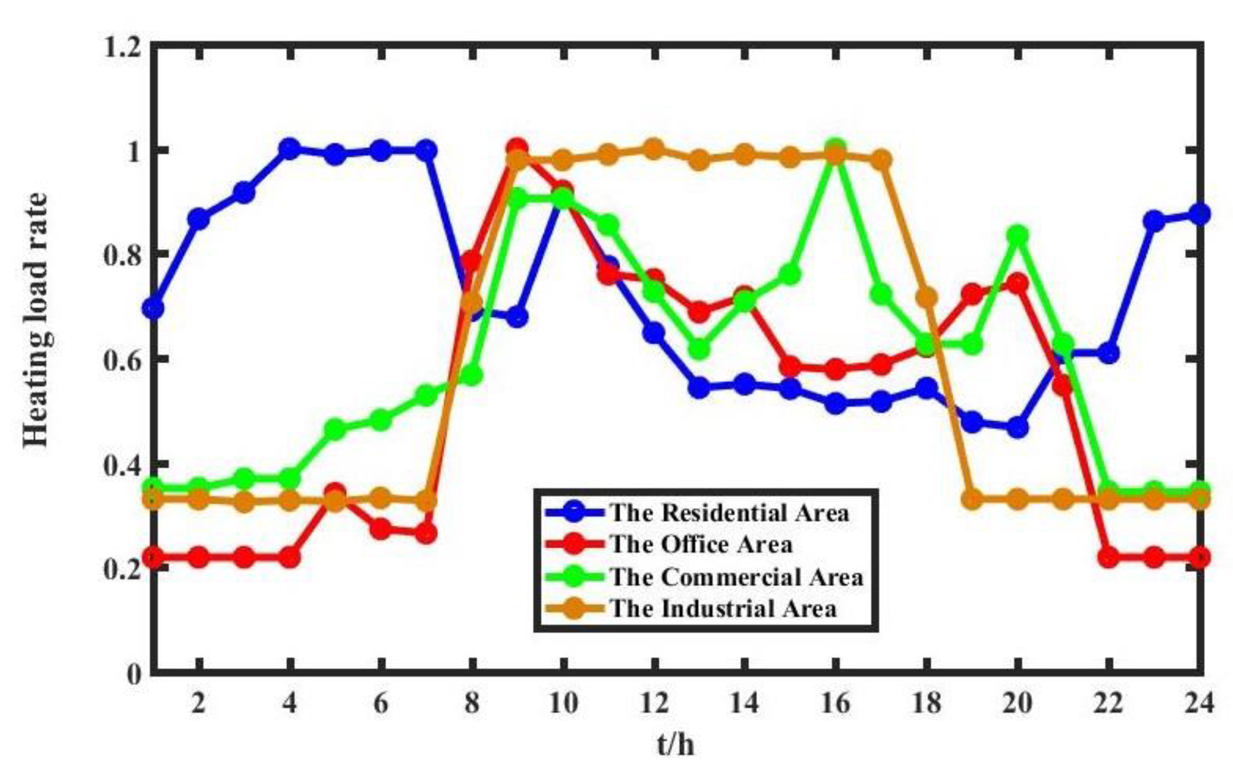
The typical heating load rate curves of multiple functional areas are shown in Figure 1. The x-axis represents 24 h of the day.

It can be seen from Figure 1 that the peak period of heating loads in the residential area occurs at night, while in the daytime it is lower, which is in line with the living habits of residents going out in the morning and going back home in the evening. In the office area, the heating loads are higher in working hours from 8 a.m. to 5 p.m., and in overtime from 6 p.m. to 9 p.m. In the commercial area, the heating loads are higher during the business period and lower during the nonbusiness period. The heating loads in the industrial area are mostly productive heating loads. The heating load rate is very high from 8 a.m. to 5 p.m. during the operation period of the factories, and relatively low at night due to the shutdown of some factories.

2.3.2. Cooling Loads

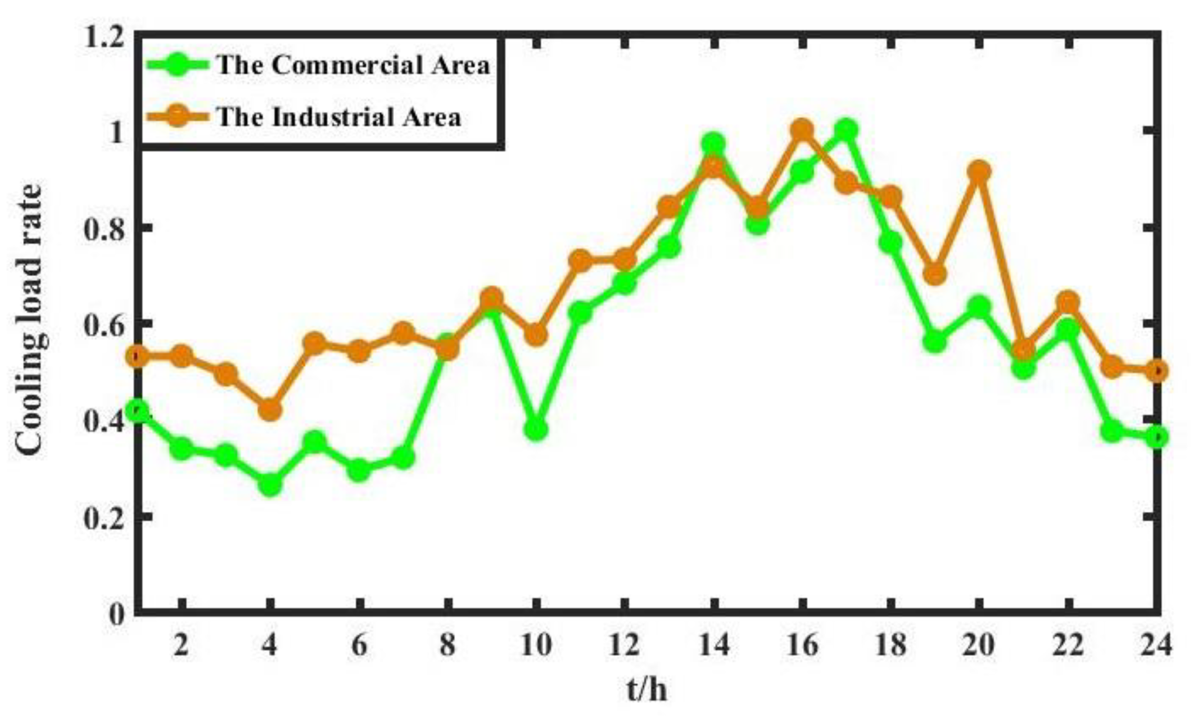
The typical cooling load rate curves of multiple functional areas are shown in Figure 2. The x-axis represents 24 h of the day.

It can be seen from Figure 2 that the cooling loads only exist in the commercial area and the industrial area, and the variation characteristics of cooling loads in these two functional areas are relatively similar. Due to the higher outdoor temperature, the cooling load rate is higher in the daytime and lower at night. The cooling load rate reaches the full day peak around 2 p.m.–4 p.m. The temperature requirement of storage cooling loads is much stricter in the industrial area than in the commercial area, which is the reason why the storage cooling load curve seems smoother in the former area.

2.3.3. Electric Loads

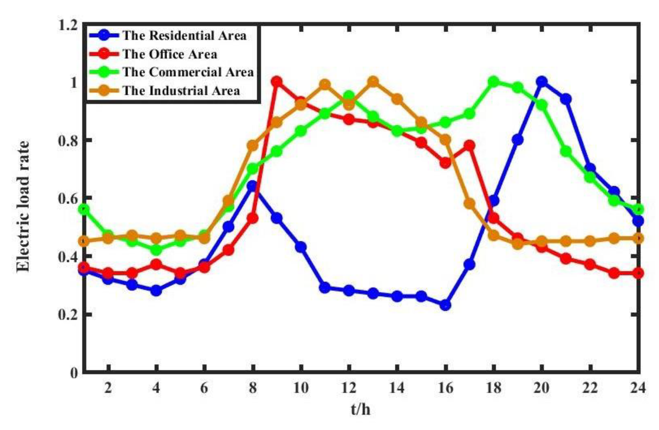
Referring to the analysis method of daily loads curves in [26], typical electrical load rate curves of the four functional areas are shown in Figure 3. The x-axis represents 24 h of the day.

It can be seen from Figure 3 that electric loads in the residential area show double peaks at 8 a.m. and 8 p.m., which are consistent with people’s habits. From 8 a.m. to 9 a.m., the electric loads rise rapidly to the peak in the office area, and decrease significantly after work at 5 p.m. The peak period of electric loads in the commercial area are 8 a.m.–9 p.m., and the electric load rate is maintained above 0.65. In periods other than business hours, the electric loads rate is maintained at a lower level. Compared with other functional areas, the industrial area has higher full-day load rate and load rate in the daytime is higher than that at night, which is consistent with the working systems of factories.

2.3.4. Charging Loads of EVs

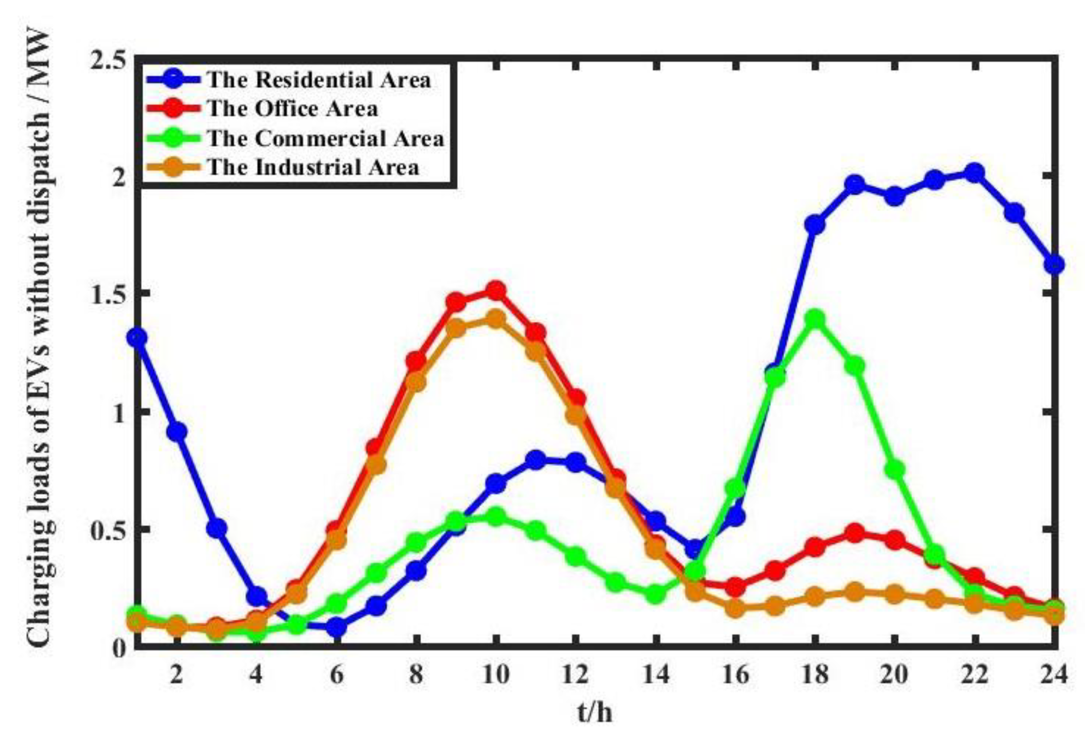
The typical predicted charging loads curves of EVs of multiple functional areas are shown in Figure 4, in which the number of EVs is assumed as 2000. The x-axis represents 24 h of the day. The Monte Carlo simulation method is adopted to simulate EVs parking, driving, and charging behavior at different times and different areas for predicting the spatiotemporal characteristics of charging loads of EVs [27].

It can be seen from Figure 4 that since residents in the residential area usually go out early and go home late, EVs are charged concentratively at night and the peak period of charging loads occur around 10 p.m. EVs in the office area are charged during working hours, usually from 8 a.m. to 5 p.m. The concentration period of load charging in the commercial area is generally 5 p.m.–9 p.m., and fast charging is taken due to the shorter parking time. Charging loads characteristics of the industrial area are similar to that of the office area, and are concentrated in the working hours from 8 a.m. to 5 p.m. for charging. However, the charging loads from 6 p.m.–9 p.m. in the industrial area are lower than that in the office area, because a small part of the office staff overworks. The number of EVs in the office area is higher than that of EVs in the industrial area during this period.

The peak of charging loads in each functional area overlaps with the peak period of electric loads of the functional area, but does not match the output curve of renewable energy in this functional area. It will not only impact the distribution network to a certain extent, but also is not conducive to the consumption of renewable energy. Thus, it is necessary to dispatch the charging loads of EVs which have flexibility and energy storage characteristics.

2.3.5. Comparisons of the Load Characteristics of Multiple Functional Areas

In summary, the load characteristics of multiple functional areas are summarized and compared in

Table 3. Comparisons of load characteristics of multiple functional areas.

Loads	Residential Area	Office Area	Commercial Area	Industrial Area
Heating Loads	High at night and low in the day, and constrained by the PMV index	High during working hours, low from the end of work hours to night, and constrained by PMV index	High during business hours, low at night, and constrained by PMV index	High during the day, relatively low at night, not subject to PMV index
Cooling Loads	Affected by the equivalent thermal resistance D	N/A	N/A	Affected by the equivalent thermal resistance D
Electric Loads	Double peaks in the morning and evening	High during working hours	Double peaks at noon and night	High loads rate throughout the day, highest during the daytime
Charging Loads of EVs	Concentrated on charging at night	Concentrated on charging during working hours	Concentrated on charging during shopping and leisure time, and with large charging power	Concentrated on charging during working hours

.

It can be seen from Table 3 that the heating loads, the cooling loads, the electric loads, and the charging loads of multiple functional areas have different characteristics. The functional areas could be connected through tie lines and the transferability of EVs to achieve complementary coordination and reduce the abandonment rate of renewable energy. The heating/cooling loads inside a functional area also have a certain flexibility and adjustability, which could be utilized to improve the consumption of renewable energy and suppress the volatility of renewable energy.

3. Coordinated Dispatching Model of IESs Considering Differences of Multiple Functional Areas

Previous work on IES system dispatching mainly focused on single-area IES. There are few studies on multiarea IES dispatching and less consideration on different load characteristics of different areas. Thus, inevitably, there were some problems, such as low energy efficiency and poor economic benefits. To solve the above problems, the different load characteristics of different functional areas are considered and the following points are proposed in this paper: (1) the cooling loads, heating loads, and charging loads of EVs have energy storage characteristics; (2) the cooling loads and heating loads are suitable for transmission within the functional areas; (3) the electric loads and charging loads of electric vehicles are suitable for transmission across functional areas. Thus, a coordinated dispatching model of IESs is established considering the above characteristics. Through the complementarity of various forms of energy systems and different loads in multiple functional areas, the absorption rate of renewable energy can be effectively improved and the economic efficiency of the operation of IESs can be improved.

Uncertainty is a key factor to be considered in power management and there is strong uncertainty in renewable energy output. Scenario analysis and robust optimization are commonly used to deal with uncertainty in power management problems. In scenario analysis, uncertainties are described through scenario sets [28]. Uncertain parameter intervals are used in robust optimization to describe the uncertainty. Robust optimization requires less information about the probability distribution of random variables [29,30,31]. Considering that scenario analysis can clearly describe the probability characteristics of uncertain variables and its optimization model can be easily calculated, scenario analysis is used to deal with production uncertainty in this paper. It is assumed that there are S scenes, and the probability of scene s is $p_s$. The lowest operating cost is generally taken as the objective of coordinated dispatching model. In order to promote the consumption of renewable energy, the cost of abandoned WT and PV power is added to the total operating cost of the IESs. Thus, the objective function of coordinated dispatching of IESs is to minimize the total operating cost of the systems, and can be represented as

$$\min {\displaystyle \sum _{s=1}^S{p}_s{\displaystyle \sum _{t=1}^T{\displaystyle \sum _{r=1}^R}}}\{{\displaystyle \sum _{i=1}^{N_{rchp}}[c_i^{\mathrm{chp}}(P_{\mathrm{chp},r,i,t}^s,H_{\mathrm{chp},r,i,t}^s)+{\rho }_1|P_{\mathrm{chp},r,i,t}^s-P_{\mathrm{chp},r,i,t}^0|]}+\phi P_{\mathrm{buy},r,t}^s+{\rho }_2|P_{\mathrm{buy},r,t}^s-P_{\mathrm{buy},r,t}^0|+{\rho }_3{P}_{\mathrm{cut},r,t}^s\}$$

(11)

$$\begin{array}{ll}{c}_i^{\mathrm{chp}}(P_{\mathrm{chp},r,i,t}^s,H_{\mathrm{chp},r,i,t}^s)=& a_{0,r,i}+a_{1,r,i}{P}_{\mathrm{chp},r,i,t}^s+a_{2,r,i}{H}_{\mathrm{chp},r,i,t}^s+a_{3,r,i}(P_{\mathrm{chp},r,i,t}^s{)}^2\\ & +a_{4,r,i}(H_{\mathrm{chp},r,i,t}^s{)}^2+a_{5,r,i}{P}_{\mathrm{chp},r,i,t}^s{H}_{\mathrm{chp},r,i,t}^s\end{array}$$

(12)

$$P_{\mathrm{cut},r,t}^s=P_{\mathrm{PW},r,t,\max }^s+P_{\mathrm{PV},r,t,\max }^s-P_{\mathrm{PW},r,t}^s-P_{\mathrm{PV},r,t}^s-P_{\mathrm{PWH},r,t}^s-P_{\mathrm{PVH},r,t}^s$$

(13)

The cost function of CHP units and the expression of abandoned WT and PV power could be described as (12) and (13), respectively.

The constraints of the subsystems in the IESs are as follows:

1. Constraints of electric systems

Constraint of the electric power balance [32] can be represented as

$${\displaystyle \sum _{i=1}^{N_{rchp}}{P}_{\mathrm{chp},r,i,t}^s}+P_{\mathrm{buy},r,t}^s+P_{\mathrm{PV},r,t}^s+P_{\mathrm{PW},r,t}^s+{\displaystyle \sum _{l=1}^{L_r}{P}_{\mathrm{tie},l,t}^s}=P_{\mathrm{L},r,t}^s+P_{\mathrm{ch},r,t}^s+P_{\mathrm{EC},r,t}^s$$

(14)

It shows that electric loads can be balanced between functional areas through tie lines and EVs.

Constraints of the CHP unit can be represented as

$$P_{\mathrm{chp},r,i,t}^s=H_{\mathrm{chp},r,i,t}^s/k_{\mathrm{hp},r,i}$$

(15)

$$P_{\mathrm{chp},r,i}^{\min }\le P_{\mathrm{chp},r,i,t}^s\le P_{\mathrm{chp},r,i}^{\max }$$

(16)

$$-U_{r,i}^{\max }\cdot \Delta t\le P_{\mathrm{chp},r,i,t+1}^s-P_{\mathrm{chp},r,i,t}^s\le U_{r,i}^{\max }\cdot \Delta t$$

(17)

The thermoelectric constraint is described as (15), the electric output constraint is described as (16), and the climbing constraint is described as (17).

Constraints of the purchasing power can be represented as

$$P_{r,t}^s\ge 0$$

(18)

It means that electric power can be purchased but not sold.

Constraints of the WT and PV can be represented as

$$P_{\mathrm{PV},r,t}^s\ge 0$$

(19)

$$P_{\mathrm{PW},r,t}^s\ge 0$$

(20)

$$P_{\mathrm{PWH},r,t}^s\ge 0$$

(21)

$$P_{\mathrm{PVH},r,t}^s\ge 0$$

(22)

$$0\le P_{\mathrm{PV},r,t}^s+P_{\mathrm{PWH},r,t}^s\le P_{\mathrm{PV},r,t,\max }^s$$

(23)

$$0\le P_{\mathrm{PW},r,t}^s+P_{\mathrm{PVH},r,t}^s\le P_{\mathrm{PW},r,t,\max }^s$$

(24)

Constraints of the tie line transmission power can be represented as

$$-P_{\mathrm{tie},l,t}^{\max }\le P_{\mathrm{tie},l,t}^s\le P_{\mathrm{tie},l,t}^{\max }$$

(25)

2. Constraints of heating systems

Constraints of the electric boiler can be represented as

$$P_{\mathrm{EB},r,t}^s=P_{\mathrm{PWH},r,t}^s+P_{\mathrm{PVH},r,t}^s$$

(26)

$$H_{\mathrm{EB},r,t}^s={\eta }_{\mathrm{EB},r}{P}_{\mathrm{EB},r,t}^s$$

(27)

$$0\le H_{\mathrm{EB},r,t}^s\le H_{\mathrm{EB},r}^{\max }$$

(28)

In order to improve the consumption rate of renewable energy, it is assumed that the electric boiler is installed in the generating stations of renewable energy, and the electric energy required by the electric boiler can only supplied by the renewable energy connected to it. It is ensured by (26) that the electric boiler in area r consumes WT and PV power in area r only. Constraints of thermoelectric conversion relations and heating output limits of the electric boiler are described in (27) and (28), respectively.

For areas where the heating loads are the ordinary heating loads, i.e., residential, office, or commercial areas, the constraints can be represented as

$${\displaystyle \sum _{i=1}^{N_{rchp}}{H}_{\mathrm{chp},r,i,t}^s}+H_{\mathrm{EB},r,t}^s=H_{\mathrm{L},r,t}^s$$

(29)

$$H_{\mathrm{L},r,t}^s={\chi }_r^s(T_{\mathrm{g},r,t}^s-T_{\mathrm{h},r,t}^s)$$

(30)

$$T_{\mathrm{h},r,t}^s\le T_{\mathrm{g},r,t}^s\le T_{\mathrm{g},r,\max }^s$$

(31)

$$-{\sigma }_{r,t}^s\le {\lambda }_{r,PMV,t}^s\le +{\sigma }_{r,t}^s$$

(32)

For areas with the productive heating loads, i.e., the industrial area, the constraints are presented in (4) and (5).

3. Constraints of cooling systems

Constraints of indoor cooling can be represented as

$$Q_{\mathrm{EC},r,t}^s=Q_{\mathrm{L},r,t}^s$$

(33)

$${\tilde{T}}_{\mathrm{n},r,\min }^s\le {\tilde{T}}_{\mathrm{n},r}^s\le {\tilde{T}}_{\mathrm{n},r,\max }^s$$

(34)

The indoor cooling constraints also include the ETP model described in (6).

Constraints of the electric refrigerator can be represented by

$$Q_{\mathrm{EC},r,t}^s=P_{\mathrm{EC},r,t}^s{\eta }_{\mathrm{EC},\mathrm{r}}$$

(35)

$$Q_{\mathrm{EC},r,\min }^s\le Q_{\mathrm{EC},r,t}^s\le Q_{\mathrm{EC},r,\max }^s$$

(36)

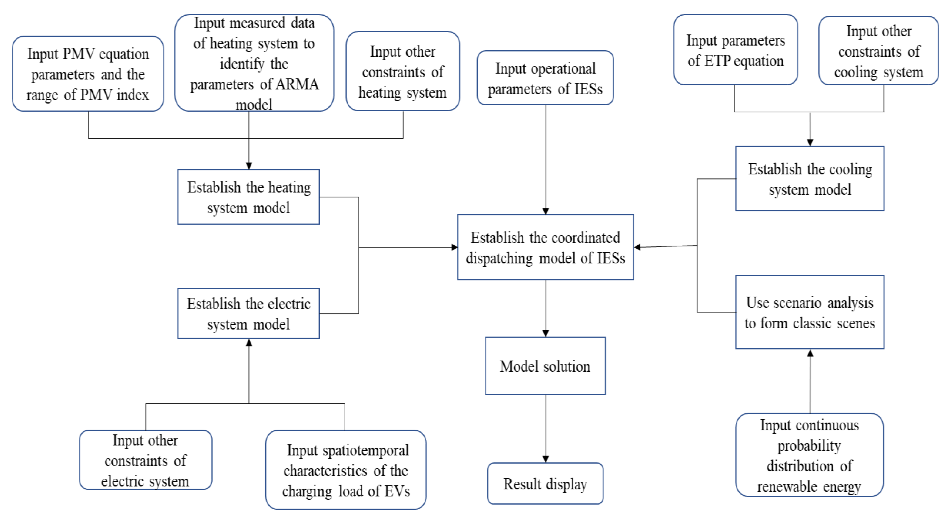
The proposed coordinated dispatching model of IESs considering differences of multiple functional areas is established using the programming software YALMIP in MATLAB, and is then solved by the commercial optimization solver CPLEX 12.6.1.

The objective function of the proposed model is a quadratic function and the constraints are linear functions, so it is a quadratic programming problem. YALMIP is a free MATLAB toolbox which can solve many optimization models, such as quadratic programming, second-order cone programming, and mixed integer programming. The greatest feature of YALMIP is that it can integrate many external optimization solvers regardless of whether these solvers are written in MATLAB or not.

CPLEX is a commercial optimization solver developed by IBM. It is specifically used to solve four basic problems: large-scale linear programming, quadratic programming, constrained quadratic programming, second-order cone programming, and corresponding mixed integer programming. CPLEX can solve some very difficult industry problems and its solving speed is very fast. With the support of CPLEX, the efficiency of MATLAB for large-scale problems and linear programming has been greatly improved.

The process of the optimization algorithm is shown in Figure 5.

4. Case Studies

Renewable energy is developing rapidly in Europe, and its installed proportion is relatively high. In view of the uncertainties and fluctuations of renewable energy and the reduction of fossil fuel power generation, Denmark has attached great importance to the development and promotion of commercially available and scalable high-performance distributed electrothermal energy systems in recent years. At present, the energy supply of Denmark mainly comes from green energy sources such as wind energy, biomass energy, and solar energy. Denmark pays attention to the interaction and complementarity between green renewable energy and energy storage systems, and combines solar, wind, and biomass energy with electric and thermal energy storage to make the whole energy system more flexible.

Taking Svendborg, Denmark as an example, there are currently three solar power stations in Svendborg. One of them has an area of 6000 m² and annual power supply of 2736 MWh. “Waste incineration and electrothermal energy storage” is one of the main sources of thermal energy supply in Svendborg at present. Local waste incinerators burn about 70,000 tons of waste annually, including food packaging, cartons, and plastics. By using the latest technology, the combustion efficiency is up to 98%. The incinerator burns at a stable high temperature of 1000 °C, which reduces the emission of harmful gases such as CO₂. Through the complementary use of various forms of energy systems, the power generation efficiency of Svendborg has reached 49%.

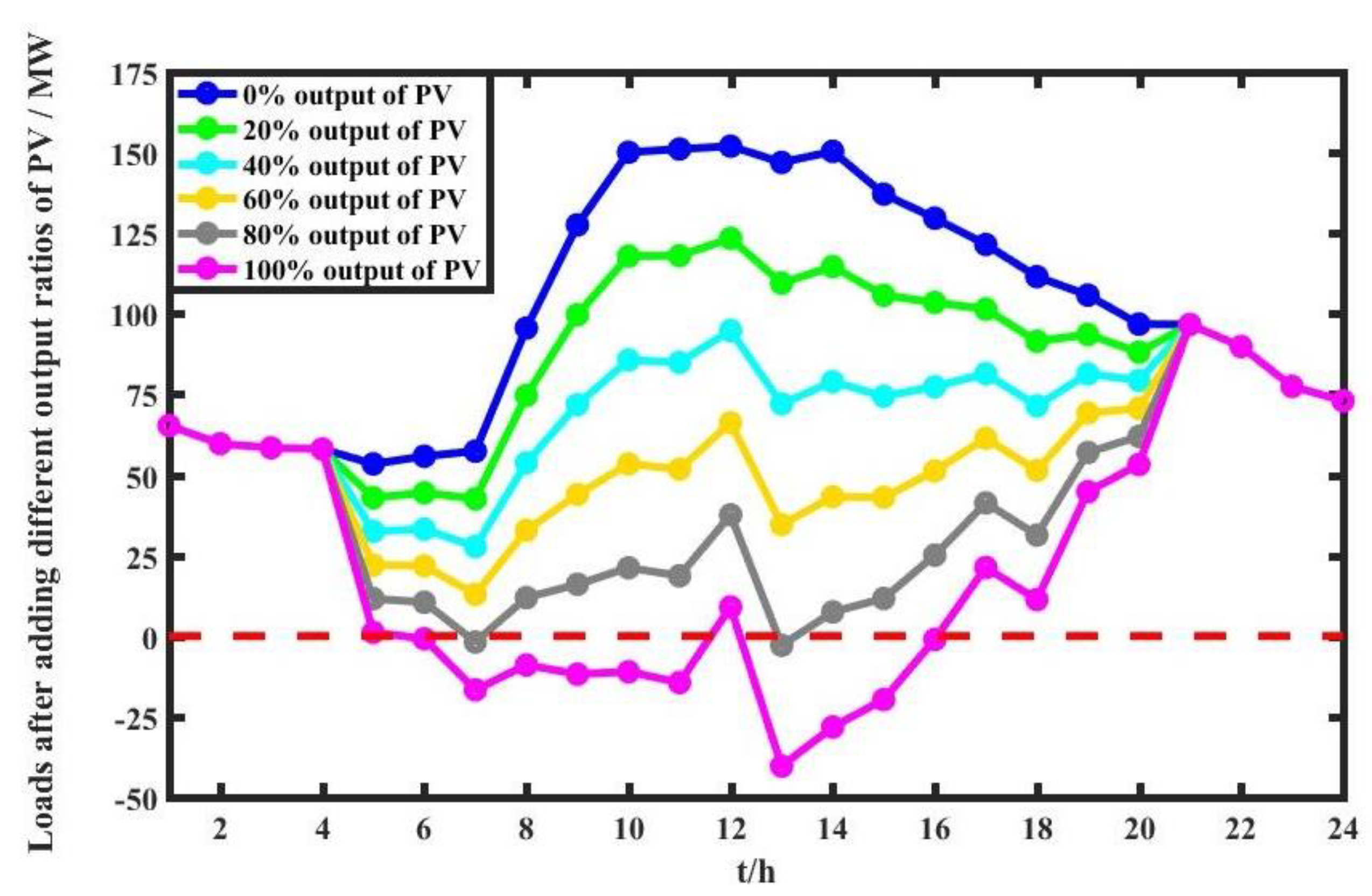
For demonstrating the effectiveness of the proposed coordinated dispatching model of IESs, an actual distribution system in Jianshan District, Haining, Zhejiang Province of China is presented. Due to many factors, such as renewable energy power generation subsidy policy, local photovoltaic panel capacity, and the effect of the demonstration zone, the installed capacity of renewable energy in Jianshan District has increased rapidly. By August 2018, the total installed capacities of grid-connected PV and WT in Jianshan District were 180 MW and 50 MW, respectively, which are expected to continue growing in the next several years. The high penetration rate of renewable energy leads to the great operating pressure for the dispatchers of the distribution network in the region. When the loads are low, the excess energy is evenly transferred to the transmission systems with high-voltage level. Taking one typical daily electrical load curve and the typical photovoltaic output data as example, the PV output can be considered as a negative load. Then, the loads with different output ratios of PV are shown in Figure 6.

It can be seen from Figure 6 that when the output ratio of PV is more than 80%, the loads after adding the output of PV are less than 0. In order to improve the power grid structure and utilize the distribution network to transfer the excess energy, the measures to be taken in Jianshan District include improving the interconnection level of distribution networks and building energy storage devices. In 2016, Zhejiang Development Planning and Research Institute issued the “Central Heating Plan of Haining”, which proposed to implement centralized heating in Haining. At the same time, Jianshan District has been clearly divided into four functional areas in the planning stage, and the development of EVs is encouraged. Under this background, the effect of coordinated dispatching of IESs considering the differences of multiple functional areas on renewable energy consumption in Jianshan District is analyzed.

The geographical distribution of functional areas in Jianshan District is shown in Figure 7, where areas 1, 2, 3, and 4 represent the residential area, the office area, the commercial area, and the industrial area, respectively. The connection between functional areas is through tie lines 1–2, 1–3, and 1–4, respectively. The positive direction of power flow in the tie line is shown by the arrows in Figure 7.

The relevant parameters of the case are listed in the Appendix A. The power capacity of each functional area is shown in

Table A1. Power capacities of multiple functional areas.

	Residential Area	Office Area	Commercial Area	Industrial Area
CHP (MW)	15	12	12	35
WT (MW)	15	0	0	35
PV (MW)	30	35	30	70

. The parameters of CHP units are shown in

Table A2. Parameters of CHP units.

Functional Areas	Maximum Power Generation/(MW)	Minimum Power Generation/(MW)	Ramp Rate/(MW/h)
Residential Area	15	3	4.5
Office Area	12	2.4	3.6
Commercial Area	12	2.4	3.6
Industrial Area	35	7	10.5

. It is assumed that there is only one CHP unit in each functional area. The parameters of EVs are shown in

Table A3. Parameters of EVs.

Time Period	Residential Area			Office Area
	$\left[P_{\mathbf{ch},r,t}^{\mathbf{min}},P_{\mathbf{ch},r,t}^{\mathbf{max}}\right]$/(MW)	$\left[{\alpha }_{r,k}^{\mathbf{min}},{\alpha }_{r,k}^{\mathbf{max}}\right]$	$E_{r,k}^{av}$/(MW·h)	$\left[P_{\mathbf{ch},r,t}^{\mathbf{min}},P_{\mathbf{ch},r,t}^{\mathbf{max}}\right]$/(MW)	$\left[{\alpha }_{r,k}^{\mathbf{min}},{\alpha }_{r,k}^{\mathbf{max}}\right]$	$E_{r,k}^{av}$/(MW·h)
8 a.m.–5 p.m.	[0,0.5]	[0.7,1.3]	2.43	[0,2]	[0.7,1.3]	1.83
6 p.m.–9 p.m.	[0,1.5]	[0.7,1.3]	3.64	[0,0.75]	[0.7,1.3]	2.43
10 p.m.–7 a.m.	[0,3]	[0.7,1.3]	11.41	[0,0.5]	[0.7,1.3]	9.71
Time Period	Commercial Area			Industrial Area
	$\left[P_{\mathbf{ch},r,t}^{\mathbf{min}},P_{\mathbf{ch},r,t}^{\mathbf{max}}\right]$/(MW)	$\left[{\alpha }_{r,k}^{\mathbf{min}},{\alpha }_{r,k}^{\mathbf{max}}\right]$	$E_{r,k}^{av}$/(MW·h)	$\left[P_{\mathbf{ch},r,t}^{\mathbf{min}},P_{\mathbf{ch},r,t}^{\mathbf{max}}\right]$/(MW)	$\left[{\alpha }_{r,k}^{\mathbf{min}},{\alpha }_{r,k}^{\mathbf{max}}\right]$	$E_{r,k}^{av}$/(MW·h)
8 a.m.–5 p.m.	[0,0.5]	[0.7,1.3]	2.43	[0,2]	[0.7,1.3]	9.71
6 p.m.–9 p.m.	[0,2.2]	[0.7,1.3]	5.47	[0,0.38]	[0.7,1.3]	0.91
10 p.m.–7 a.m.	[0,0.5]	[0.7,1.3]	2.43	[0,0.5]	[0.7,1.3]	2.43

. The operating parameters of the IES are shown in

Table A4. Operating parameters of the IES.

${\mathit{a}}_{0,1}$/($)	$a_{1,1}$/($/(MW·h))	$a_{2,1}$/($/(MW·h))	$a_{3,1}$/($/(MW·h)2)	$a_{4,1}$/($/(MW·h)2)	$a_{5,1}$/(($/(MW·h)2)
1650	1450	420	345	30	31
$\phi$/($/(MW·h))	${\rho }_1$/($/(MW·h))	${\rho }_2$/($/(MW·h))	${\rho }_3$/($/(MW·h))	$k_{hp}$	$P_{r,l}^{\mathbf{max}}$/(MW)
550	60	50	100	2.62	5
$H_{\mathbf{EB},1}^{\mathbf{max}}$/(MW)	$H_{\mathbf{EB},2}^{\mathbf{max}}$/(MW)	$H_{\mathbf{EB},3}^{\mathbf{max}}$/(MW)	$H_{\mathbf{EB},4}^{\mathbf{max}}$/(MW)	${\eta }_{r,\mathbf{EB}}$	${\chi }_1$/(MW/°C)
25	15	15	35	0.9	0.55
${\chi }_2$/(MW/°C)	${\chi }_3$/(MW/°C)	$T_{r,g,\mathbf{max}}$/(°C)	$Q_{\mathbf{EC},3,\mathbf{min}}$/(MW)	$Q_{\mathbf{EC},3,\mathbf{max}}$/(MW)	$Q_{\mathbf{EC},4,\mathbf{min}}$/(MW)
0.45	0.35	120.0	0	20	0
$Q_{\mathbf{EC},4,\mathbf{max}}$/(MW)	${\tilde{T}}_{\mathbf{n},3,\mathbf{min}}$/(°C)	${\tilde{T}}_{\mathbf{n},3,\mathbf{max}}$/(°C)	${\tilde{T}}_{\mathbf{n},4,\mathbf{min}}$/(°C)	${\tilde{T}}_{\mathbf{n},4,\mathbf{max}}$/(°C)	D/(°C/MW)
30	−18.0	−10.0	−20.0	−15.0	2
C/(MW·h/°C)	${\eta }_{\mathbf{EC},\mathbf{r}}$	$\lambda$	${\mu }_1$	${\mu }_2$	-
0.54	3.0	0.3	0.8	1.2	-

. The parameters of the PMV index are shown in

Table A5. Parameters of the PMV index.

M/(W/m2)	W/(W/m2)	$P_{\mathbf{a}}/\mathbf{\left(}\mathbf{Pa}\mathbf{\right)}$	$t_{\mathbf{b}}/$(°C)
70.0	0.0	2000.0	29.7
$t_{\mathbf{cl}}$/(°C)	$f_{\mathbf{cl}}$	$h_{\mathbf{c}}$/(W/(m2·K))	-
32.0	1.15	4.7	-

. The coefficients of the ARMA model of heating systems are shown in

Table A6. Coefficients of the ARMA model of heating systems (J = 2).

$\mathit{j}$	${\mathit{\alpha }}_{\mathit{j}}$	${\mathit{\beta }}_{\mathit{j}}$	${\mathit{\gamma }}_{\mathit{j}}$	${\mathit{\theta }}_{\mathit{j}}$	${\mathit{\phi }}_{\mathit{j}}$	${\mathit{\omega }}_{\mathit{j}}$
0	—	0.2112	0.3317	—	—	—
1	0.5721	−0.0243	−0.3169	0.6991	0.1011	0.1998
2	0.0607	−0.0104	0.1741	—	—	—

. The initial values of the heating/cooling systems are shown in

Table A7. Initial operation values of heating/cooling systems.

$T_{\mathbf{g},0}^{}$/(°C)	$T_{\mathbf{g},-1}^{}$/(°C)	$T_{\mathbf{n},0}^{}$/(°C)	$T_{\mathbf{n},-1}^{}$/(°C)
75.0	75.0	25.0	25.0
$T_{\mathbf{w},0}$/(°C)	$T_{\mathbf{w},-1}$/(°C)	${\tilde{T}}_{\mathbf{n}0,3}$/(°C)	${\tilde{T}}_{\mathbf{n}0,4}$/(°C)
0.0	0.0	−10.0	−10.0

. It is assumed that the heating systems of each functional area have the same initial value of operation. The typical daily loads and outdoor temperature data of each functional area in winter are shown in

Table A8. Typical daily loads and outdoor temperature data of multiple functional areas in winter.

Time	Electric Loads of Residential Area/(MW)	Electric Loads of Office Area/(MW)	Electric Loads of Commercial Area/(MW)	Electric Loads of Industrial Area/(MW)	Outdoor Temperature/(°C)
1	17.74	7.70	11.03	34.85	−2.0
2	13.62	7.43	10.24	33.88	−2.0
3	12.38	7.15	9.45	34.85	−2.0
4	11.55	7.15	8.93	35.82	−4.0
5	10.73	6.16	6.72	34.85	−4.0
6	12.38	5.72	7.14	35.82	−4.0
7	14.44	5.94	7.56	34.85	−4.0
8	19.39	17.6	14.45	53.01	−2.0
9	24.75	22.00	22.26	70.29	−1.0
10	20.63	41.80	24.36	77.21	0.0
11	16.50	39.05	26.46	82.97	3.0
12	11.14	37.40	28.56	88.74	4.0
13	10.73	36.30	30.24	82.97	7.0
14	10.32	35.75	28.14	89.88	7.0
15	9.90	34.65	21.17	84.13	7.0
16	9.90	33.00	21.50	77.21	8.0
17	9.08	30.25	21.84	71.45	8.0
18	14.44	32.45	22.85	51.85	7.0
19	22.69	17.60	31.92	42.64	5.0
20	30.94	9.63	31.50	32.91	5.0
21	38.78	9.08	23.52	33.88	2.0
22	36.30	8.25	19.49	33.88	1.0
23	27.23	6.16	17.14	33.88	−1.0
24	23.93	5.72	15.12	34.85	−1.0

. The continuous probability distribution of unit WT and PV is shown in

Table A9. The continuous probability distributions of WT/PV.

Time	WT/(MW)	PV/(MW)
1	N(0.707, 0.1362)	0
2	N(0.769, 0.1502)	0
3	N(0.862, 0.1882)	0
4	N(0.923, 0.1862)	0
5	N(0.785, 0.2142)	N(0.267, 0.1402)
6	N(0.662, 0.1992)	N(0.289, 0.1452)
7	N(0.554, 0.1892)	N(0.378, 0.1392)
8	N(0.400, 0.1432)	N(0.533, 0.2062)
9	N(0.600, 0.2402)	N(0.711, 0.2802)
10	N(0.569, 0.2412)	N(0.822, 0.3342)
11	N(0.585, 0.2782)	N(0.844, 0.3462)
12	N(0.600, 0.2852)	N(0.956, 0.3522)
13	N(0.600, 0.2922)	N(0.956, 0.3992)
14	N(0.508, 0.2642)	N(0.911, 0.3972)
15	N(0.538, 0.2732)	N(0.800, 0.3342)
16	N(0.508, 0.2702)	N(0.667, 0.3602)
17	N(0.415, 0.2252)	N(0.511, 0.2802)
18	N(0.462, 0.2232)	N(0.511, 0.2782)
19	N(0.554, 0.2942)	N(0.311, 0.1572)
20	N(0.615, 0.2972)	N(0.222, 0.1172)
21	N(0.723, 0.3092)	0
22	N(0.600, 0.2672)	0
23	N(0.692, 0.2632)	0
24	N(0.800, 0.3122)	0

.

4.1. The Optimization Results of Coordinated Dispatching for an Integrated Energy System

The population of Jianshan District is about 100,000, and the penetration rate of EVs is taken as 2%, that is, the number of EVs is 2000; the charging coefficient ${\alpha }_{r,k}^{\min }$ is taken as 0.7, the PMV index is taken as 0.5, the adjustable heating duration T’ is taken as 3, the capacity of each tie line is taken as 5 MW, and the equivalent thermal resistance D is taken as 2. Thus, the optimization of coordinated dispatching for the integrated energy system can be performed.

The correlation between the output of renewable energy and the charging power of EVs in each functional area is analyzed, and the results are shown in

Table 4. Correlation coefficients between the output of renewable energy and the charging power of EVs in each functional area.

Time Period	Residential Area	Office Area	Commercial Area	Industrial Area
8 a.m.–5 p.m.	0.7411	0.6709	0.5345	0.6548
6 p.m.–9 p.m.	0.7642	0.4455	0.5482	0.7979
10 p.m.–7 a.m.	0.6885	N/A	N/A	0.7447

.

It can be seen from Table 4 that the correlation coefficient between the output of renewable energy and the charging power of EVs in each functional area is positive, indicating that the charging power of EVs and the output of renewable energy are synchronously changed. The larger the output of renewable energy, the larger the charging power of EVs will become, which provides a larger consumption margin for renewable energy. Thus, the correlation coefficient in the area with rich renewable energy, such as the residential area and the industrial area, is also significantly larger. During 10 p.m.–7 a.m., the correlation coefficient and the output of renewable energy in the industrial area is the largest, but EVs are concentrated in the residential area. In order to increase the consumption rate of the renewable energy in the industrial area during this period, it is possible to reduce the charging price of the industrial area during this period so that more EVs could be charged in this area. During 6 p.m.–9 p.m., EVs are concentrated in the commercial area, but the correlation coefficient is small. This is because the parking time of EVs in this time period is short, and in this short parking time, the owners of EVs prefer to utilize the fast charging mode to meet their charging requirements, rather than responding to dispatching instructions to consume excess renewable energy. Thus, the commercial area should not set too many charging piles, and it is better to transfer this part of the charging demand to other periods or other areas.

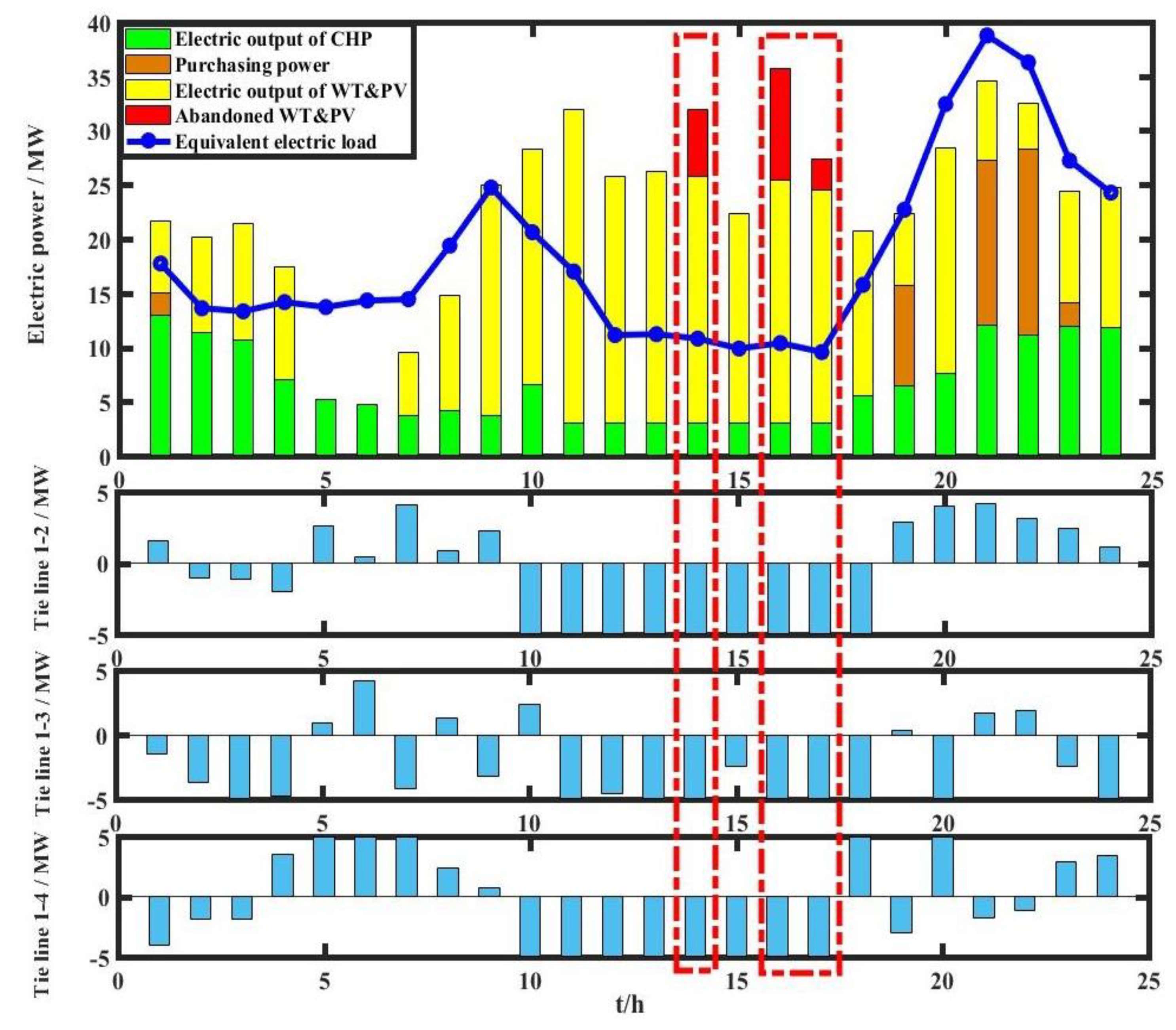
For analyzing the optimization of electric power and tie line power in a certain scene, the residential area is taken as an example for demonstration, and the result is shown in Figure 8. The equivalent electric loads are the electric loads superimposed with the charging loads of EVs. It can be seen from Figure 8 that since PV power is the major renewable energy in the residential area and the loads of the daytime are low, the renewable energy is excessive in the daytime, and it should be transmitted through three tie lines. There is abandoned WT and PV power at 2 p.m., 4 p.m., and 5 p.m. This is because the three tie lines connected to the residential area have reached the limitation of transmission.

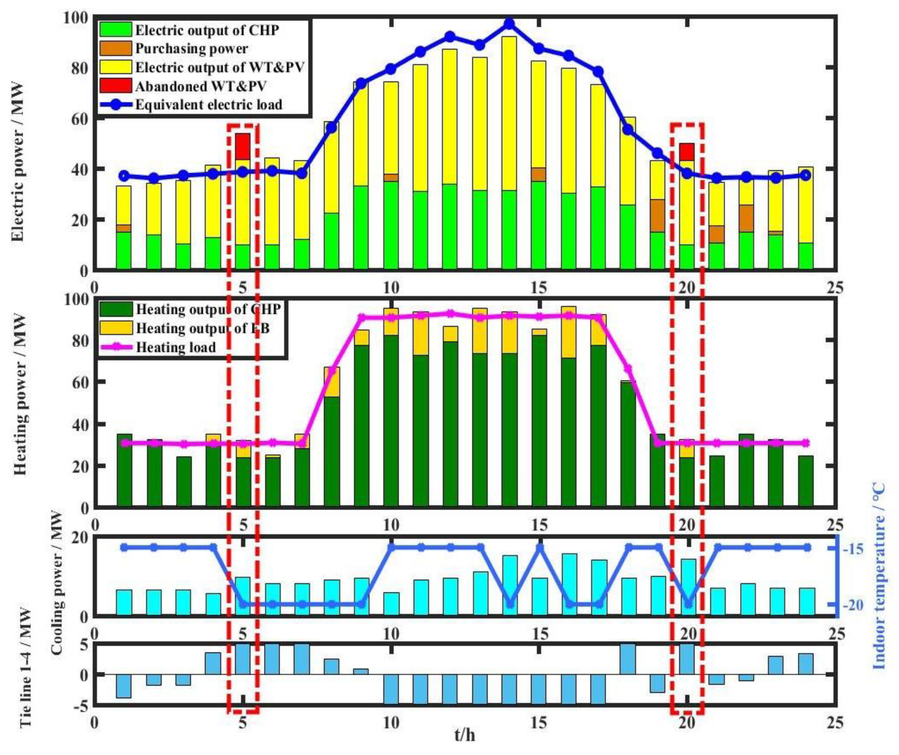
Furthermore, the industrial area is also taken as an example for analyzing the optimization of the cooling power, the heating power, the electric power, and the tie line power, which is shown in Figure 9. The equivalent electrical loads are the electric loads superimposed with the charging loads of EVs. It can be seen from Figure 9 that there is abandoned WT and PV power at 5 a.m. and 8 p.m. During this period, the CHP unit has reached its minimum technical output, providing the largest consumption margin of renewable energy. Meanwhile, the heating power is 31.77 MW and 32.17 MW at 5 a.m. and 8 p.m., respectively. The heating load is 30.15 MW and 30.55 MW at 5 a.m. and 8 p.m., respectively. The heating power has exceeded the heating load in the allowable range of the heat elasticity at 5 a.m. and 8 p.m. to consume more renewable energy. The cooling power during this period is larger than the adjacent periods, and the indoor temperature of the cooling building has reached −20°C, which is the lowest temperature in allowance. The tie line has also reached the limitation of the transmission power. The abandonment rate of WT and PV power has been minimized through the coordination optimization of cooling power, heating power, electric power, and tie line power.

4.2. The Impacts of the Penetration Rate of EVs and the Charging Coefficient on the Consumption of Renewable Energy

The impacts of the penetration rate of EVs on the consumption of renewable energy are compared and analyzed, and the results for different penetration rates of EVs are shown in

Table 5. Abandoned WT and PV power in functional areas under different penetration rates of EVs.

Penetration Rate of EVs	Abandoned WT and PV power in Residential Area/(MW)	Abandoned WT and PV power in Industrial Area/(MW)
2%	12.73	18.37
6%	9.66	15.63
10%	6.88	14.29

. Since there is no abandoned WT and PV power in both the office area and the commercial area, only abandoned WT and PV power in the residential area and the industrial area are listed. It can be seen from Table 5 that the abandoned WT and PV power in the residential area and the industrial area are also decreasing with the increase of the penetration rate of EVs, while the reduction of the residential area is more obvious. The reason is that the number of EVs distributed in the residential area is greater than the industrial area during the periods of abandoned WT and PV power, so the penetration rate of EVs have a greater impact on the consumption of renewable energy in the residential area than in the industrial area. In summary, transferring the charging loads of EVs in the industrial area to the periods with abandoned WT and PV power by reducing the charging price in these periods should be considered.

The impacts of the charging coefficient ${\alpha }_{r,k}^{\min }$ on the consumption of renewable energy are compared and analyzed, and the results for different charging coefficients are shown in

Table 6. Abandoned WT and PV power in functional areas under different charging coefficients.

${\mathit{\alpha }}_{\mathit{r},\mathit{k}}^{\mathbf{min}}$	Abandoned WT and PV power in Residential Area/(MW)	Abandoned WT and PV power in Industrial Area/(MW)
0.7	12.73	18.37
0.4	11.03	17.95
0	10.88	17.67

. Since there is no abandoned WT and PV power in both the office area and the commercial area, only abandoned WT and PV power in the residential area and the industrial area is listed in Table 6. It can be seen from Table 6 that with the decrease of ${\alpha }_{r,k}^{\min }$, the abandoned WT and PV power in the residential area and the industrial area is also decreasing, because ${\alpha }_{r,k}^{\min }$ relates to the minimum charging power in time period k of area r. When ${\alpha }_{r,k}^{\min }$ decreases, the lower limit of charging power could be more relaxed, which means that EVs can be charged in other time periods and other areas. Thus, the charging power of EVs could match the output curves of renewable energy better, and the abandoned power of renewable energy could be reduced.

4.3. The Impacts of the Capacity of Each Tie Line on the Consumption of Renewable Energy

The impacts of tie line capacity on the consumption of renewable energy are compared and analyzed in

Table 7. Abandoned WT and PV power in functional areas under different tie line capacities.

Capacity of Each Tie Line/(MW)	Abandoned WT and PV power in Residential Area/(MW)	Abandoned WT and PV power in Industrial Area/(MW)
5	12.73	18.37
8	1.58	11.28
10	0	7.54

. Since there is no abandoned WT and PV power in both the office area and the commercial area in various situations, only abandoned WT and PV power in the residential area and the industrial area is listed in Table 7. It can be seen from Table 7 that when the tie line capacity is increased, the abandoned WT and PV power in the residential area and the industrial area is decreasing, while the reduction of the residential area is more obvious. Because the electric loads and the heating loads of the residential area are not high during the daytime, the output of PV in the residential area is relatively high during this period, and the excess power of PV could be transmitted to other functional areas where the electric loads and heating loads are relatively high through the three tie lines. Therefore, the consumption rate of renewable energy in the residential area has been significantly improved with the increase of the capacity of tie lines.

There is abandoned WT and PV power during 5 a.m.–7 a.m. in the industrial area, and the electric loads, the heating loads, and the cooling loads of other functional areas are not high and the output of renewable energy of other functional areas is rich during this period. Meanwhile, there is only one tie line in the industrial area, so the renewable energy cannot be completely consumed through the tie line. In summary, the tie line capacity of the industrial area could be expanded or tie lines between the industrial area and other functional areas could be established to reduce the abandonment of WT and PV power in the industrial area.

4.4. The Impacts of the PMV Index and the Adjustable Heating Duration on Heating Systems

The impacts of the PMV index on heating systems are compared and analyzed in

Table 8. Abandoned WT and PV power in functional areas under different PMV indexes.

PMV Index	Abandoned WT and PV power in Residential Area/(MW)	Abandoned WT and PV power in Office Area/(MW)
0.2	13.68	0.75
0.5	12.73	0
1	2.20	0

. Since the PMV index is not suitable for evaluating the heating loads of the industrial area and there is no abandoned WT and PV power in the commercial area, only the abandoned WT and PV power in the residential area and the office area are listed in Table 8. Taking the residential area as an example, the heating loads curves and indoor temperature curves under different PMV indices are shown in Figure 10.

Figure 10a shows the output curve of WT and PV power of the residential area in a specific scenario. Figure 10b,c show the heating loads power curves and the indoor temperature curves of the heating building under different PMV index in this scene, respectively. The dotted lines in Figure 10c are the allowed range of indoor temperature fluctuations under the corresponding PMV index. It can be seen from Table 8 that as the PMV index becomes stricter, the abandoned WT and PV power in the residential area increases and there is abandoned WT and PV power in the office area when the PMV index is 0.2. This is because the stricter the PMV limit is, the smaller the range of indoor temperature fluctuations, and the smaller the elasticity of the heating loads on the amplitude axis is, resulting in a reduction in the virtual ‘heat storage’ capacity of the heating systems. Therefore, in the case of large fluctuations in renewable energy, it cannot work well to stabilize and consume renewable energy. In the residential area, the output of WT and PV is large during 8 a.m.–5 p.m. and abandoned WT and PV power appears during this period. When the PMV index is widened, the heating loads during this period can be increased and the indoor temperature is increased to the upper limit within the allowed range, thus allowing consumption of renewable energy. In summary, the restriction of the PMV index could be relaxed to reduce the abandonment rate of WT and PV.

As for the industrial area, some industries could adjust their working time to alter the heating duration T’ across a wider time range. The impacts of T’ on the consumption of renewable energy are compared and analyzed in

Table 9. Abandoned WT and PV power in the industrial area under different adjustable heating durations.

T’	Abandoned WT and PV power in Industrial Area/(MW)
3	18.37
6	15.32
9	12.14

. It can be seen from Table 9 that when T’ is increased, the abandoned WT and PV power of the industrial area decreases. Therefore, if heating supply could be adjusted at a larger time scale, more renewable energy could be consumed.

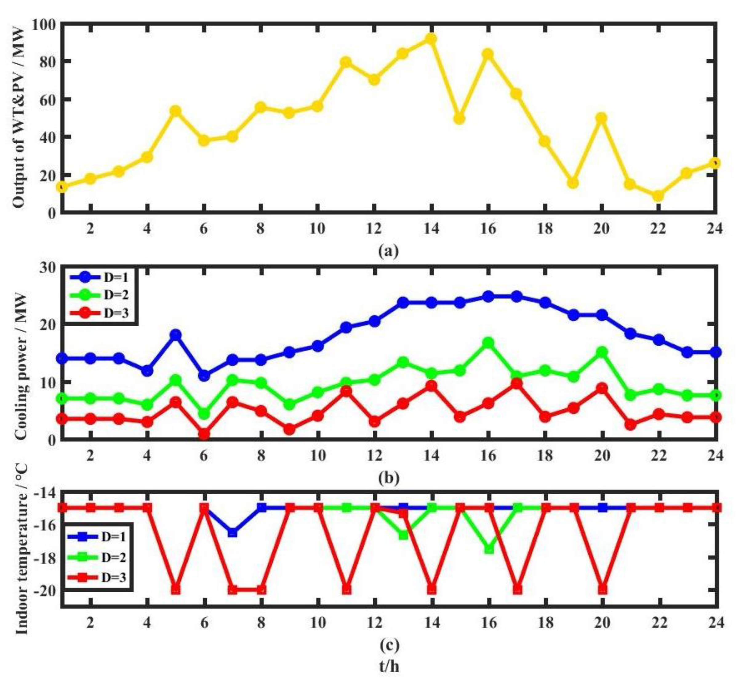
4.5. The Impacts of Equivalent Thermal Resistance on Cooling Systems

The impacts of the equivalent thermal resistance D on cooling systems are analyzed. According to the characteristics of different cooling buildings, the equivalent thermal resistance D is taken as 1 and 3, respectively. Taking the industrial area as an example, the cooling load curves and indoor temperature curves under different equivalent thermal resistance D are demonstrated in Figure 11. The correlation coefficients between the output of renewable energy and the cooling power under different equivalent thermal resistance are shown in

Table 10. Correlation coefficients between the output of renewable energy and the cooling power.

D	Correlation Coefficient
1	0.5585
2	0.5741
3	0.6237

.

Figure 11a shows the output curve of WT and PV of the industrial area in a certain scenario. Figure 11b and Figure 11c show the cooling loads curves and the indoor temperature curves of the cooling building under different equivalent thermal resistances D in this scene, respectively. The value of D represents the degree of the influence of the indoor temperature in the previous period on the indoor temperature in the latter period. It can be seen from Figure 11b that the larger D is, the better the effect of the cooling systems on the cold energy storage is and the smaller the required cooling loads are. As shown in Figure 11c, when D is larger, the cooling systems are more inclined to lower the indoor temperature, and the cold inertia is utilized to ‘store energy’; when D is smaller, the cooling systems are more inclined to just meet the cooling temperature requirements. It can be seen from Figure 11 and Table 10 that when D becomes larger, the change of the cooling load is more synchronized with the changes of WT and PV. In summary, cooling buildings with a larger equivalent thermal resistance D could be utilized to reduce the volatility of renewable energy.

5. Conclusions

Different characteristics of the cooling loads, heating loads, electric loads, and charging loads of EVs of multiple functional areas are analyzed. Then, a coordinated dispatching strategy for integrated energy systems considering the differences of multiple functional areas and various forms of energy systems is presented, in which the connection between the functional areas is established through tie lines and EVs. The balance of the cooling loads and the heating loads is realized within each functional area. In the proposed coordinated dispatching strategy, the elasticity and inertia of heating/cooling load are also considered to exert the energy storage function of the heating/cooling loads. Moreover, the impacts of these factors on the consumption of renewable energy and the suppression of the volatility of renewable energy are given. Finally, an actual distribution system in Jianshan District, Haining, Zhejiang Province of China was used to demonstrate the effectiveness of the proposed coordinated dispatching model of integrated energy systems. The simulation results show that it is conducive to consuming the excess renewable energy and suppressing the volatility of renewable energy by improving the penetration rate of EVs, tie line capacity, equivalent thermal resistance, and adjustable heating duration, and properly releasing the PMV restriction and the charging power restriction of EVs.

It should be mentioned that the model of this paper could be further studied under the following conditions: (1) A more detailed model of the heating network could be considered, including heating delay and loss, etc.; (2) The cost of tie lines could be considered to find the most suitable tie line capacity; (3) The distribution characteristics of EVs in various functional areas could be changed through the factor of electricity price to achieve more optimized dispatching without improving the penetration rate of EVs.