Analysis of the Guide Vane Jet-Vortex Flow and the Induced Noise in a Prototype Pump-Turbine

Featured Application

This work provides a way to visualize the pressure pulsation signal in turbomachinery flow case. It can be also used in all the engineering CFD cases.

Abstract

The start-up process of a pump-turbine in pump mode is found with obvious noise, especially at the small guide vane opening angle. The turbulent-flow-induced noise is an important part and must be reduced by flow control. Therefore, the computational fluid dynamics (CFD) method is used in this study to predict the internal flow in a high head prototype pump-turbine (the specific speed n_q is 31.5) under an extremely off-design condition (C_φ = 0.015 and C_α = 0.096). The acoustic analogy method is also used to predict the near-field noise based on the turbulence field. Special undesirable flow structures including the flow ring between the runner trailing-edge and the guide vane, guide vane jet, twin-vortexes adjacent to guide vane jet, inter stay vane vortex, stay vane jet, and volute vortex-ring are found in a pump-turbine. These complex jet-vortex flow structures induce local high turbulence kinetic energy and an eddy dissipation rate, which is the reason why noise is generated at small guide vane opening angle. Three dominating frequencies are found on the turbulence kinetic energy pulsation. They are the runner blade frequency f_b = 64.5 Hz, the dominate frequency in the guide vane and the stay vane f_gsv = 9.6 Hz, and the dominate frequency in volute f_vl = 3.2 Hz. The flow pulsation tracing topology gives a good visualization of frequency propagation. The dominating regions of the three specific frequencies are clearly visualized. Results show that different flow structures may induce different frequencies, and the induced specific frequencies will propagate to adjacent sites. This study helps us to understand the off-design flow regime in this prototype pump-turbine and provides guidance when encountering the noise and stability problems during pump mode’s start-up.

1. Introduction

A reversible pump-turbine is the key component in pumped storage power station [1]. It has complex varying operation conditions due to frequent starting and stopping [2]. The rotating runner, adjustable guide vane, and stay vane may cause strong rotor-stator interaction and stalled flow [3,4]. Undesirable flow regimes, including secondary flow, vortex, back flow, and submerged jet flow, could occur inside a pump-turbine [5,6,7]. The noise induced by undesirable flow structures is one of the bad factors occurring during operation [8]. It also represents a part of the energy dissipation [9]. During the operation of the prototype pump-turbine, high intensity noise is often found, especially in the pump mode’s start-up process with a small guide vane opening angle. When focusing on this noise phenomenon, complex sources can be found, including flow-induced noise and mechanical noise [10]. The mechanical noise can be reduced by conducting better design and manufacturing. However, the flow-induced noise is more complex to handle. There are different types of flow-induced noise—mainly, the turbulent-flow-induced noise [11] and the cavitation bubble collapse noise [12]. The turbulent-flow-induced noise exists in almost all the flow conditions and needs specific studies.

In bladed turbomachinery, the acoustic topic has received long-time extensive investigations [13,14,15]. For numerical simulations, there are two main ways to predict the flow-induced noise. One is the direct solving of the Navier-Stokes equations. This is accurate but requires a high computer cost. Another one is the acoustic analogy method [16]. This predicts the near-field by the computational fluid dynamics (CFD) method and extends to the far-field by computational acoustic (CA) method. Based on the methods above, researchers conducted numerical studies for the acoustic characters in bladed turbomachinery. It was found that the rotor-stator interaction could induce flow noise [17]. The distance between rotor and stator would strongly affect the noise intensity [18]. A rotating stall cell was also proved as one of the source of flow noise [19,20]. The jet flow was found as another local high noise region [21,22]. The blade exit wake also generated noise due to periodic shedding [23,24]. Generally, the local flow regime is complex in turbomachinery and may cause the noise problem.

In this study, a prototype reversible pump-turbine was studied on its turbulent-flow field and induced noise during pump mode’s start-up. Proudman [25] introduced the simulation method of turbulent-flow-induced noise, considering the turbulence isotropic assumption. Based on a prediction of the turbulence kinetic energy and dissipation rate, the local sound power distribution can be evaluated [26]. The reason for turbulent-flow-induced noise in a pump-turbine can be clarified in detail. As a widely-used, robust, and accurate method, CFD simulation is useful for predicting the turbomachinery flow cases. Currently, a lot of CFD based studies have been conducted in the pump-turbines for the flow regime [27,28], performance [29,30], cavitation [31], and stability problems [32,33]. These numerical results were compared with the tests and proved reliable and convenient. In this case, CFD simulation was used for the prototype pump-turbine. The partial-load condition with a small guide vane opening angle during pump mode’s start-up was studied. The noise caused by the special jet-vortex flow regime and its transient variation is discussed in detail. As a difficult issue in hydraulic turbomachinery flow cases, the flow mechanism at the off-design condition is also discussed in this study. The results provide a basis for understanding the flow noise and energy dissipation at partial-load in pump mode. It also reveals the flow complexity when a pump-turbine operates off-design. The relationship between the operation condition and the turbulent flow regime is also clarified. This will help the noise reduction, loss reduction, and efficiency enhancement of reversible pump-turbines.

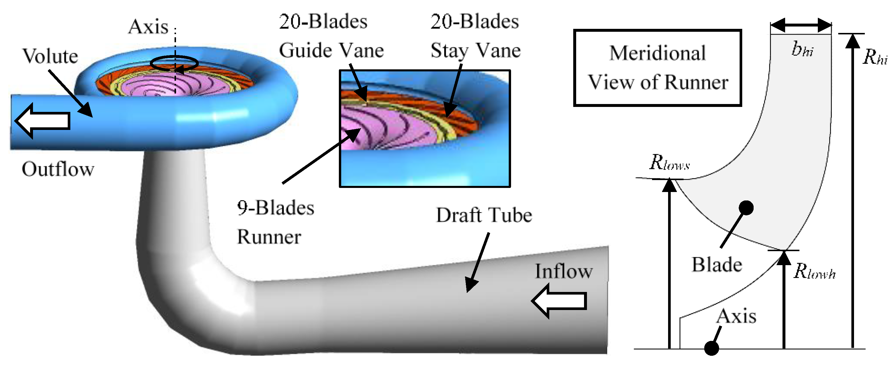
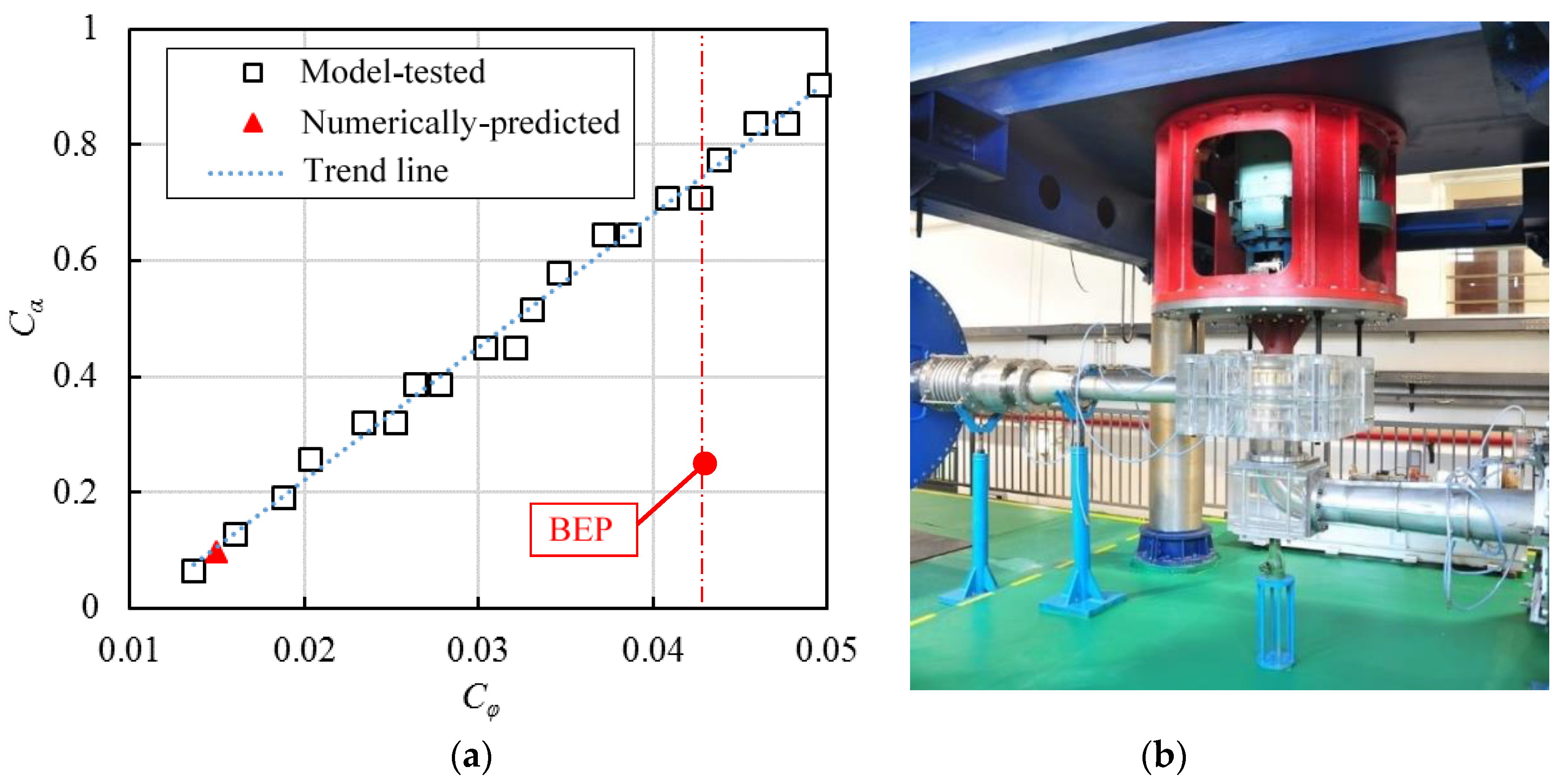
2. Pump-Turbine Unit

2.1. Parameters of Pump-Turbine

Figure 1 is the schematic map of the pump-turbine (fluid domain in prototype scale) which consists of the draft tube, runner, guide vane, stay vane, and volute. Fluid, as indicated by the vector, flows from the draft tube side to volute side in pump mode for water storage. The runner rotates in the clockwise direction in this view by n_d = 430 r/min. As shown in the meridional view, the radius at runner high pressure side is R_hi = 2.08 m. The radii at runner low pressure side R_lows (at shroud) and R_lowh (at hub) are 1.12 m and 0.64 m, respectively. The width at runner outlet b_hi is 0.4 m. The blade number of the runner, guide vane, and stay vane are 9, 20, and 20, respectively. Based on the turbomachinery similarity, the specific speed of runner n_q can be calculated by:

$$n_q=\frac{n_d\sqrt{Q_d}}{H_d^{3/4}}$$

(1)

where Q_d is the best efficiency point (BEP) flow rate and H_d is the BEP head. In this case, the specific speed n_q is equal to 31.5.

2.2. Studied Condition

A partial-load condition in pump mode is numerically studied in this case. It is indicated in Figure 2 based on the model-tested high efficiency on-cam C_φ-C_α conditions. C_φ is the flow rate coefficient which can be expressed as:

$$C_{\phi }=\frac{Q}{\pi \omega R_{hi}^3}$$

(2)

where Q is the flow rate and ω is the rotational angular speed. C_α is the relative guide vane opening angle which can be defined as:

$$C_{ \alpha }=\frac{\alpha }{{\alpha }_{max}}$$

(3)

where α is the guide vane opening angle and α_max is the maximum guide vane opening angle of 31 degrees. According to Figure 2, this numerically studied condition is about 35% of the best efficiency flow rate condition (C_φBEP = 0.043). The guide vane opening angle is about 9.6% of the maximum value. This studied condition, C_φ = 0.015 and C_α = 0.096, is in the pump mode’s start-up process which may have a complex internal flow regime and strong flow instability. CFD is used to predict the turbulent-flow-induced noise and analyze the mechanism in detail. For convenience, this studied condition is denoted as C₁ in the following sections.

3. Mathematical Modeling

3.1. Governing Equations

In this numerical case, the three-dimensional incompressible viscous flow was considered by solving the Reynolds-averaged Navier-Stokes (RANS) equations. The continuity equation and momentum equation can be written as:

$$\frac{\partial \overline{u_i}}{\partial x_i}=0$$

(4)

$$\rho \frac{\partial \overline{u_i}}{\partial t}+\rho \overline{u_j}\frac{\partial \overline{u_i}}{\partial x_j}=\frac{\partial }{\partial x_j}\left(-\overline{p}{\delta }_{ij}+2\mu \overline{S_{ij}}-\rho \overline{u_i^{\prime }{u}_j^{\prime }}\right)$$

(5)

where u velocity, t is time, ρ is density, x is coordinate component, δ_ij is the is the Kroneker delta, and μ is the dynamic viscosity. $\overline{\varphi }$ and ${\varphi }^{\prime }$ are the averaged and fluctuating components of arbitrary variable. $\overline{S_{ij}}$ is the mean rate of strain tensor:

$$\overline{S_{ij}}=\frac{1}{2}\left(\frac{\partial \overline{u_i}}{\partial x_j}+\frac{\partial \overline{u_j}}{\partial x_i}\right)$$

(6)

3.2. Turbulence Modeling

To close the RANS equations, eddy viscosity μ_t can be used to build the relationship between Reynolds stress ρ$\overline{u_i^{\prime }{u}_j^{\prime }}$ and the mean rate of strain tensor by:

$$-\rho \overline{u_i^{\prime }{u}_j^{\prime }}=2{\mu }_t\overline{S_{ij}}-\frac{2}{3}k{\delta }_{ij}$$

(7)

where k is the turbulence kinetic energy. The shear stress transport model based Detached Eddy Simulation (SST-DES) method is used for turbulent flow modeling. It is a zonal hybrid method [34] based on the Reynolds-averaged Navier-Stokes (RANS) equations and Large-Eddy Simulation (LES) equations. The SST model is used as the turbulence model for the time-averaged equations [35]. In the SST model, the turbulence kinetic energy k equation and specific dissipation rate ω equation can be specified as:

$$\frac{\partial \left(\rho k\right)}{\partial t}+\frac{\partial \left(\rho u_{i}k\right)}{\partial x_i}=P-\frac{\rho k^{3/2}}{l_{k-\omega }}+\frac{\partial }{\partial x_i}\left[\left(\mu +{\sigma }_k{\mu }_t\right)\frac{\partial k}{\partial x_i}\right]$$

(8)

$$\frac{\partial \left(\rho \omega \right)}{\partial t}+\frac{\partial \left(\rho u_i\omega \right)}{\partial x_i}=C_{\omega }P-\beta \rho {\omega }^2+\frac{\partial }{\partial x_i}\left[\left({\mu }_l+{\sigma }_{\omega }{\mu }_t\right)\frac{\partial \omega }{\partial x_i}\right]+2\left(1-F_1\right)\frac{\rho {\sigma }_{\omega 2}}{\omega }\frac{\partial k}{\partial x_i}\frac{\partial \omega }{\partial x_i}$$

(9)

where l_k-ω is the turbulence scale, which can be expressed as:

$$l_{k-\omega }=k^{1/2}{\beta }_k\omega ,$$

(10)

in which P is the production term, C_ω is the coefficient of the production term, F₁ is the blending function, and σ_k, σ_ω, and β_k are the model constants. In the DES method, the term min(l_k-ω, C_DESΔ_m) is used instead of simple l_k-ω term where Δ_m = max(Δx, Δy, Δz) is the mesh length scale, which is the maximum side length of an mesh element. If l_k-ω<C_DESΔ, the LES model will be used instead of the RANS model for modeling the turbulence flow field.

As widely known, turbulent flow in turbomachinery is mainly anisotropic. The SST model and other eddy viscosity models are based on the turbulence isotropic assumption. It can be somehow correct in engineering cases, but it lacks accuracy, especially in modeling local secondary flows. Corrections or improvements can be supplied for eddy viscosity models to have a better simulation. Therefore, DES is used to have a better solution of the jet and vortex flow field in this study. It may improve the simulation mainly in the large scale eddies. By predicting the Reynolds number (about 2.8 × 10⁶) and approximately calculating the upstream freestream velocity at the draft tube inlet (about 1.2 m/s), one is able to solve out the viscous length scale (about 0.017 mm). On one hand, the largest longitudinal eddy scale is about 30~300 times the viscous length scale. It is from about 0.5 mm to about 5 mm. On the other hand, the eddy scale of turbulence kinetic energy dissipation is about 4~8 times of the viscous length scale. It is about 0.066~0.132 mm. Considering the balance computation cost and accuracy, the DES model is mainly used for resolving the 0.5~5 mm eddies by applying a suitable mesh length scale Δ_m. The effectiveness of DES will be checked and discussed after analyzing the results.

3.3. Acoustic Analogy Method

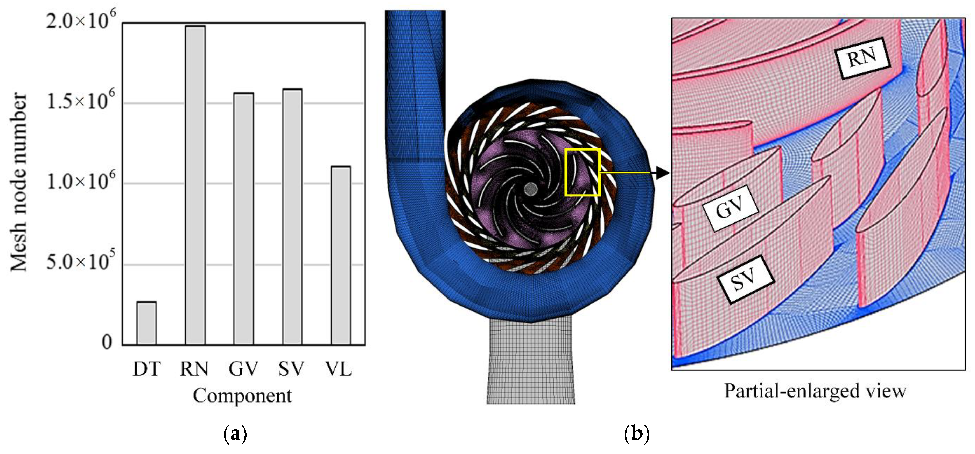
In this case, the acoustic analogy method [25,36] was used based on turbulence modeling by calculating the near-field of turbulent-flow-induced sound power W_A as:

$$W_A={\alpha }_{\epsilon }\rho \epsilon {\left(\frac{\sqrt{2k}}{V_c}\right)}^5$$

(11)

where α_ε is a constant of 0.1, ε is the eddy dissipation rate, and V_c is the sound speed in fluid medium. The turbulent-flow-induced sound power level L_sp can be calculated by:

$$L_{sp}=10{\log }_{10}\left(\frac{W_A}{W_{ref}}\right)$$

(12)

where W_ref is the reference sound power. In this study, water at 20 °C was used as the fluid medium so that V_c was 1500 m/s and W_ref was about 6.7 × 10⁻¹⁹ W/m³.

4. CFD Setup

Based on the fluid domain shown in Figure 1, the computational fluid dynamics (CFD) simulation was conducted using the commercial code CFX in ANSYS (v18, Pittsburgh, PA, USA). The mesh used in the CFD simulation was done by using ICEMCFD with structural hexahedral elements and checked in size and in y⁺. The mesh size was checked by using the grid convergence index (GCI) method [37] at the condition C₁. The pressure difference between the volute outlet and draft tube inlet was selected as the index. Three mesh schemes with 1′062′882, 2′813′808, and 6′511′958 nodes were GCI-checked with the discretization uncertainty of 5.5%, which is smaller than the limit of acceptance limit of 10% [37]. Thus, the final mesh scheme had 6′511′958 nodes to balance the accuracy and the computational cost. The y⁺ value on all the walls was controlled between 0.27 and 9.13 for applying the automatic wall-function [38] by refining the near-wall first layer height. The detail of mesh node number is shown in Figure 3. To capture the complex undesirable flow regime, especially from the runner outlet to the stay vane outlet, the mesh node density in these regions were specifically refined.

The multiple reference frame (MRF) model [39] was used where the draft tube, guide vane, stay vane, and volute were stationary, and the runner was rotational by n_d = 430 r/min. The fluid medium, which is mentioned above, was set as water at 20 °C, with a molar mass of 18.02 g/mol, density of 997 kg/m³, dynamic viscosity of 8.899 × 10⁻⁴ kg/m·s. The environment pressure was set as 1 Atm. The boundary conditions are given as follows:

• A velocity inlet boundary was given at the draft tube inflow with uniformly distributed value.
• A static pressure outlet boundary of 0 Pa was given at the volute outflow.
• No-slip wall boundaries were given on all the solid walls.
• Interfaces were set for connecting different domains based on the general grid interface method. The “frozen rotor” type was used for the rotor-stator interface in steady state simulations. The “transient rotor stator” type was used for transient simulations.

Both the steady state and transient simulations were conducted. The steady state simulation was the initial simulation by 600 steps. It converged based on the criterion of root-mean-square (RMS) residuals of the continuity and momentum equations of less than 1 × 10⁻⁵. The transient simulation was based on the steady state results. More than 5 runner revolutions were simulated. In one runner revolution, 720 time steps were conducted. At most, 10 iterations were allowed for the convergence of each time step based on the convergence criterion of RMS residuals of less than 1 × 10⁻⁶. The discrete form of the advection term in both the momentum equation and the turbulent transport equation were set as high resolution. Based on the guide vane opening angle law shown in Figure 2, the mesh scheme and numerical setup above were verified by comparing them with the model-test. Because the internal flow regime is unable to capture in model-test, the efficiency η was chosen for verification. The numerical C_φ-η data was compared with experimental C_φ-η data, as shown in Figure 4. The 4 compared conditions include the objective condition C₁, the best efficiency condition, another partial-load condition, and another over-load condition. The same tendency can be observed. It proves that the mesh scheme and numerical setup is somehow reliable for flow mechanism analysis.

5. Results and Analysis

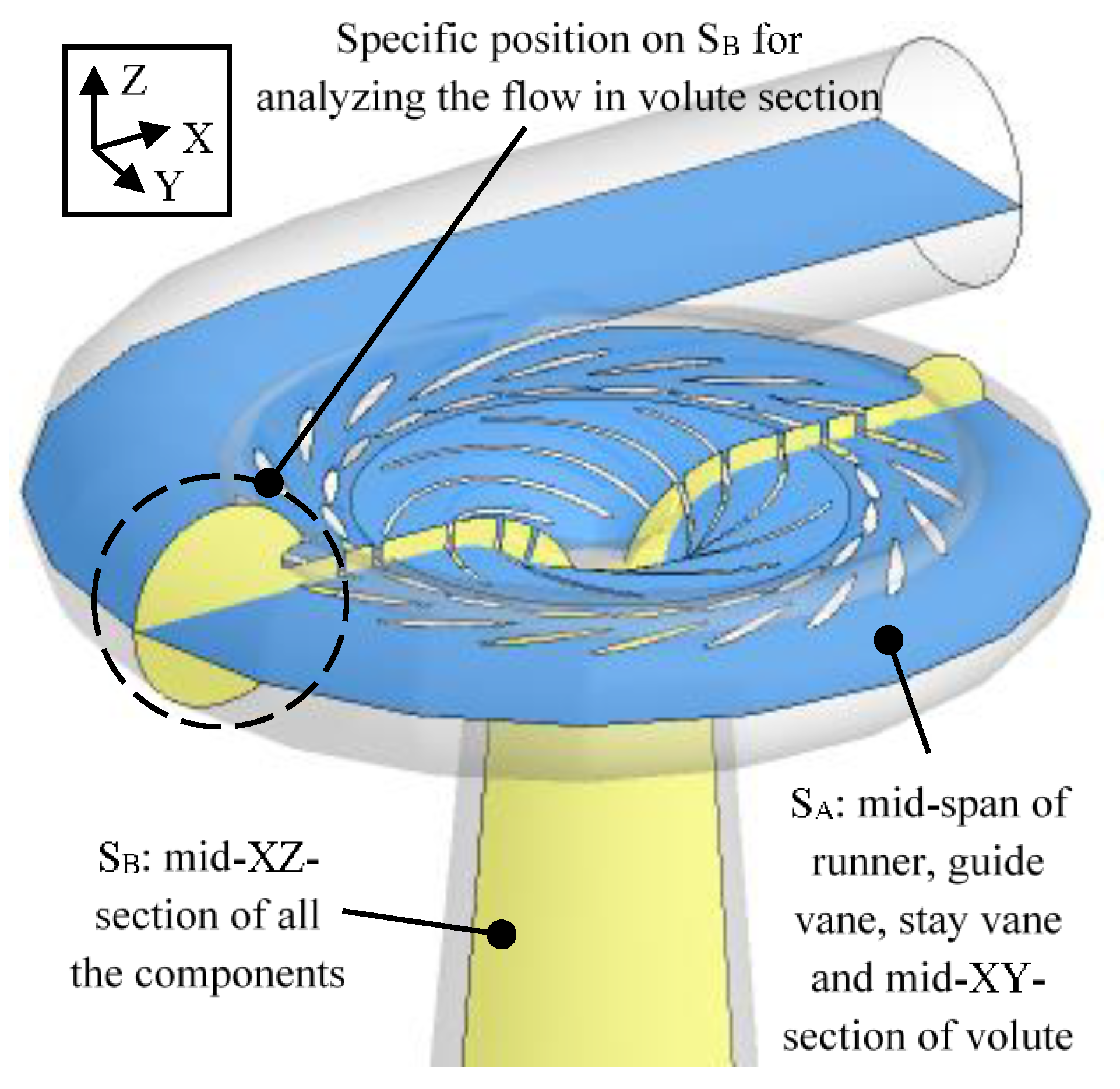
5.1. Reference Positions for Post-Processing

To analysis the internal flow regime at condition C₁, two reference surfaces were built, as shown in Figure 5 based on the XYZ orthogonal coordinate. Surface S_A includes the mid-span of the runner, guide vane, stay vane, and mid-XY-section of volute. Surface S_B is the mid-XZ-section of all the components. The specific position on S_B is also indicated for analyzing the flow on the volute section.

5.2. Internal Flow Regime

Figure 6 shows the flow regime on S_A by plotting the C_v vectors where C_v is the velocity coefficient:

$$C_{ v}=\frac{V_{rel}}{U_{hi}}$$

(13)

where V_rel is the relative velocity and U_hi is the rotational linear velocity at R_hi.

As indicated by the vectors and numbers Ⅰ–Ⅶ, there are seven special flow regimes on S_A. Number Ⅰ is the flow ring between the runner trailing-edge and guide vane. Due to the small guide vane opening angle, the passing ability is poor at condition C₁. However, the runner is continually pumping with the full rotation speed of 430 r/min. Therefore, most of the pumped water cannot pass through the guide vane but can keep rotating as a water ring there.

The guide vane jet is denoted by number Ⅱ. Numbers Ⅲ and Ⅳ are the twin-vortexes adjacent to the jet. Because of the runner pumping, some water passes through the guide vane leakage and is generated as a high-speed jet. The guide vane jet hits on the stay vane blade and causes two individual vortexes on the two sides. The vortex number Ⅲ rotated clockwise, which is the same as the runner rotation direction. On the contrary, the vortex number Ⅳ rotates counter-clockwise.

Number Ⅴ is the inter stay vane vortex, which occupies almost the entire stay vane channel. However, a stay vane jet flow denoted as number Ⅵ can be observed along the concave surface of the stay vane surface. After the guide vane jet hits on the stay vane blade, it keeps going, generates as the stay vane jet and passes through the stay vane channel. Then, the stay vane jet flow flows into the volute with high-speed.

Number Ⅶ is the volute vortex-ring. The generation of the vortex-ring can be observed in Figure 7b on surface S_B. There are two symmetrical rotating flow structures in volute. The two rotating flow structures interfere with each other and block the stay vane outlet. However, the high-speed stay vane jet can go across the vortex-ring and divides the vortex-ring into individual parts. As shown in Figure 7a, the stay vane jet flows into the volute. The two symmetrical rotating flow structures still exist.

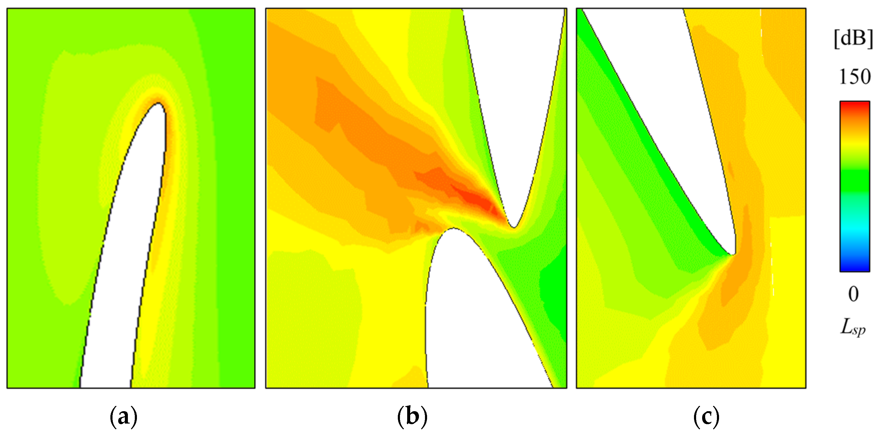
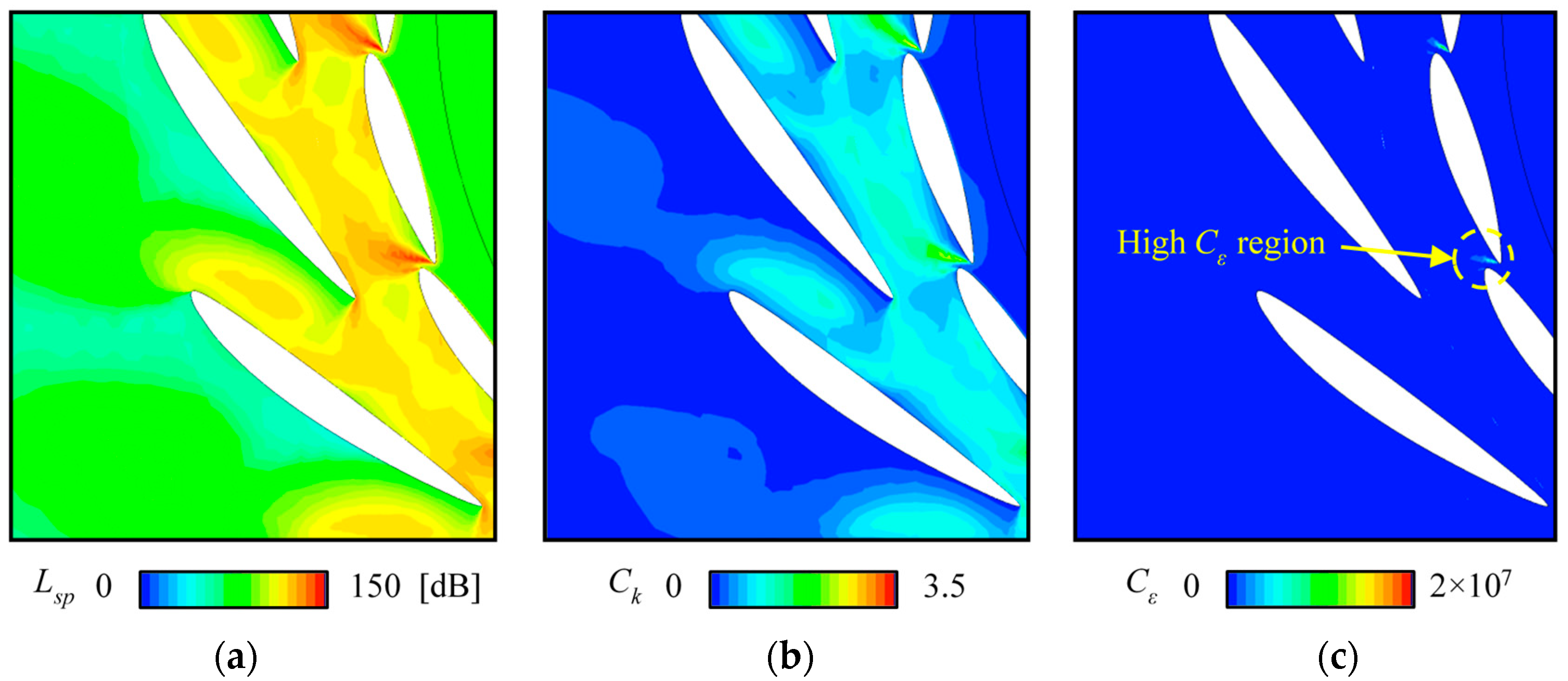
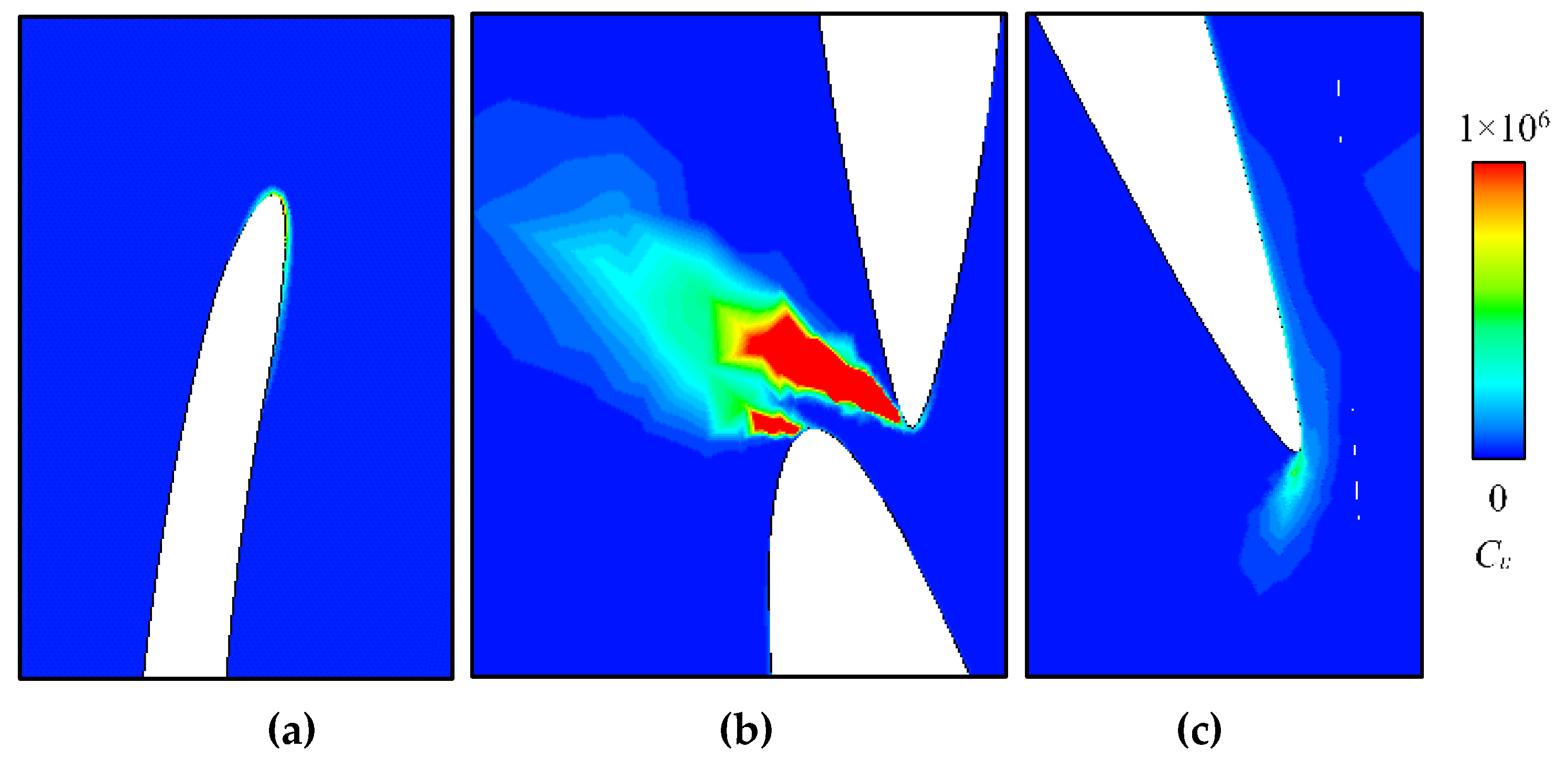
5.3. Instaneous Turbulent-Flow-Induced Noise Field

Based on the S_A and S_B surfaces, the instaneous turbulent-flow-induced noise fields were analyzed. Figure 8 shows the instaneous turbulent-flow-induced noise field on S_A by plotting the L_sp contour. The indication numbers Ⅰ to Ⅶ are kept on this figure. In the number Ⅰ region in which the flow ring is between the runner trailing-edge and the guide vane, the L_sp value is around 80 dB. This is not a high noise region. The guide vane jet region number Ⅱ is the highest L_sp region on S_A. The value of L_sp is up to 150 dB. In the twin-vortexes region numbers Ⅲ and Ⅳ, L_sp becomes higher to about 100~120 dB. However, a low L_sp value lower than 90 dB can be also observed in the vortex core region of number Ⅳ. This means that the clockwise rotating vortex produces more noise than the counter-clockwise rotating vortex. The inter stay vane vortex number Ⅴ and the stay vane jet flow number Ⅵ are also high L_sp regions. The local highest L_sp value is in the stay vane vortex core region and reached about 130 dB. The value of L_sp in the volute vortex ring number Ⅶ region decreases to about 80~100 dB. However, it is also higher than in the other parts of volute. Based on Figure 9b, it can be seen that the local highest L_sp value is in the volute vortex core region. If the stay vane jet flows across the volute vortex ring, the local highest L_sp region disappears. L_sp is relatively high on the symmetry axis due to upper-lower flow interference.

Local high L_sp regions can be also found on the runner blade leading-edge, even if there is no obvious undesirable flow pattern. Figure 10 indicates the L_sp contours on the runner blade leading-edge, guide vane blade leading-edge, and stay vane blade leading-edge. Similarities can be found in that the leading-edge regions are all in high L_sp. Specifically, two high L_sp regions can be found on one guide vane blade’s leading-edge and on another guide vane blade’s trailing-edge. On the contrary, the inter guide vane region where jet flow already generates is low in L_sp. Thus, the local flow striking and separation are the reasons why flow noise generates.

According to Equation (11), the turbulent-flow-induced noise strongly relates to the turbulence kinetic energy k and eddy dissipation rate ε. To understand the reason why noise is generated in turbulent flow, the distribution of k and ε can be studied. The dimensionless turbulence kinetic energy coefficient C_k is used:

$$C_{ k}=\frac{k}{2g{R}_{hi}}$$

(14)

where g is the acceleration of gravity. The dimensionless eddy dissipation rate coefficient C_ε is defined as:

$$C_{ \epsilon }=\frac{{\epsilon }^2}{g^3{R}_{hi}}$$

(15)

The square value of ε is used because k and ε² contribute to the same extent in predicting the turbulence-induced-noise using Equation (11). Figure 11 shows the comparison of L_sp, C_k, and C_ε contours.

Based on Figure 11, it can be found that the C_k distribution is similar to the L_sp distribution. This means that the turbulence kinetic energy strongly influences the near-field noise in pump-turbine. A high C_ε region can be also found in the guide vane jet flow region. However, the high C_ε region is very small in area. Figure 12 shows the C_ε contours on the runner, guide vane, and stay vane leading-edges in a reduced range of C_ε = 0~1×10⁶. In the reduced C_ε range, high C_ε regions can be observed on the leading-edges and almost overlap the high L_sp regions in Figure 10.

Generally, the point of view that high flow noise is strongly related to the flow regime has been proven in this study. The turbulence-induced-noise in vortex is mainly affected by turbulence kinetic energy k. For the vortex core region on the number Ⅲ, Ⅴ and Ⅶ sites, noise increases in the vortex core. For the vortex core region on number Ⅳ site, noise decreases in the vortex core. The turbulence-induced-noise in leading-edge separation regions is jointly affected by turbulence kinetic energy k and eddy dissipation rate ε. Hence, the turbulence kinetic energy k, which is physically the RMS value of fluctuating velocity, plays the most important role in inducing noise. Further analysis on the transient characteristic of k field is necessary.

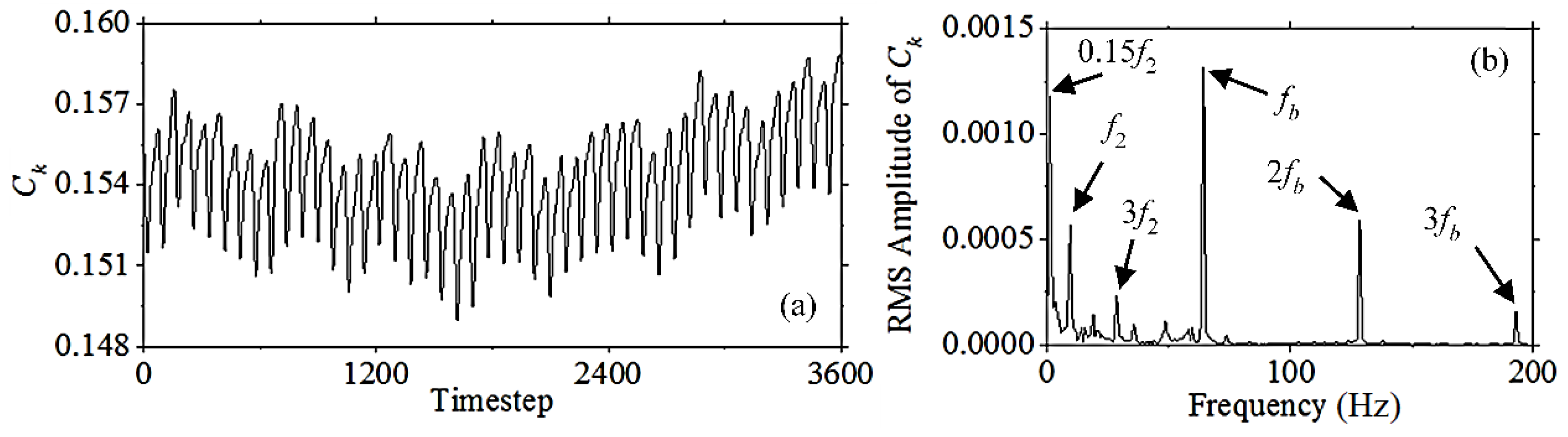
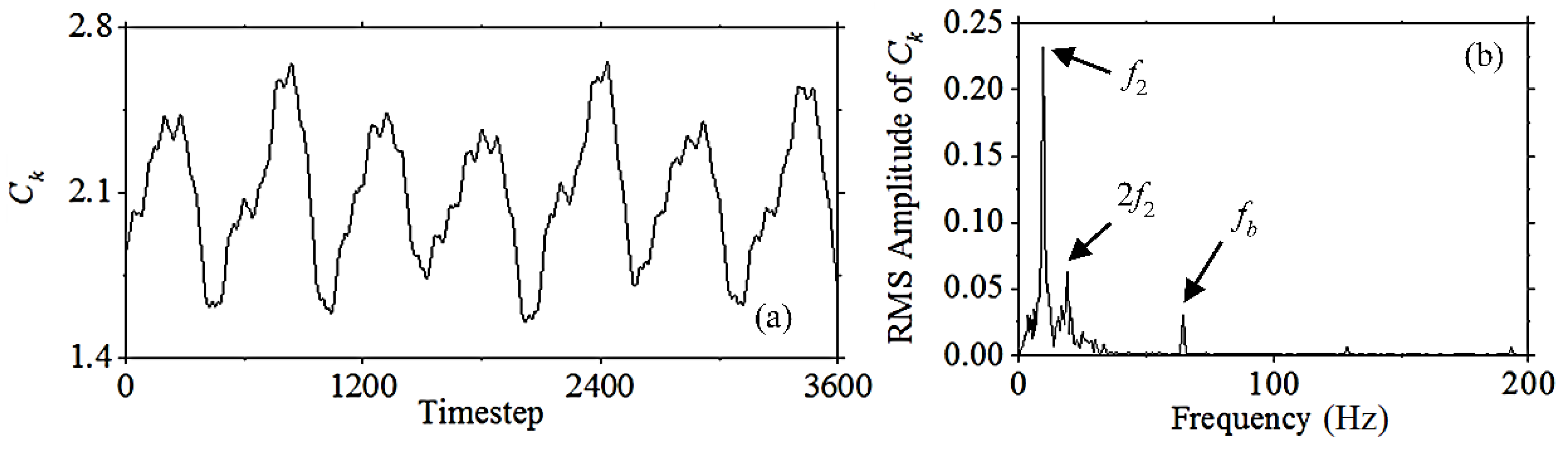
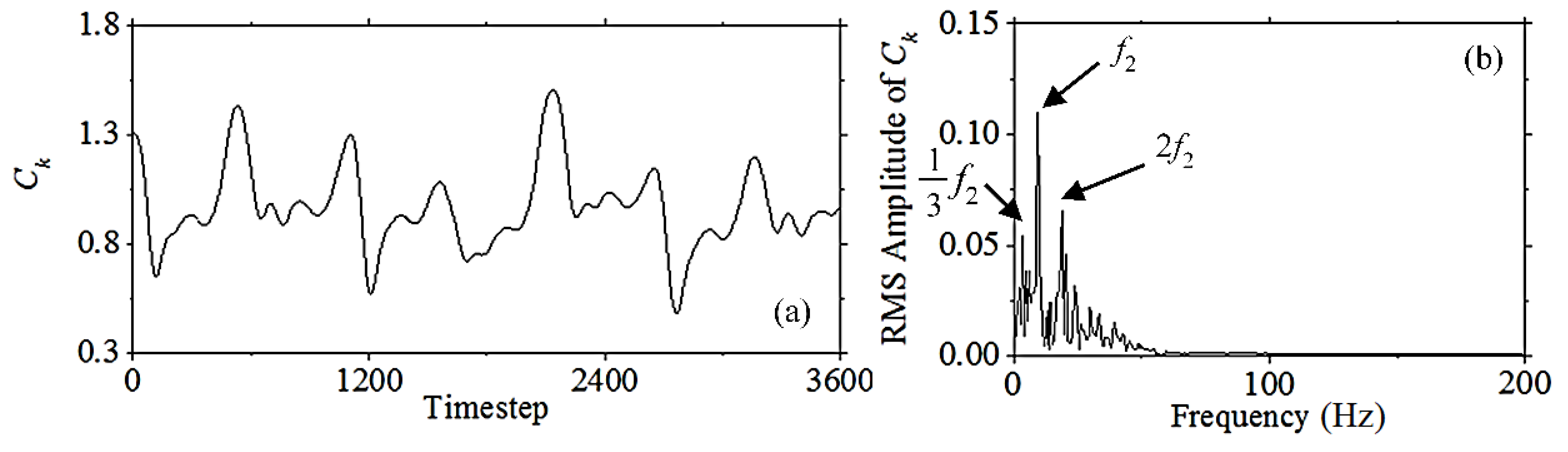
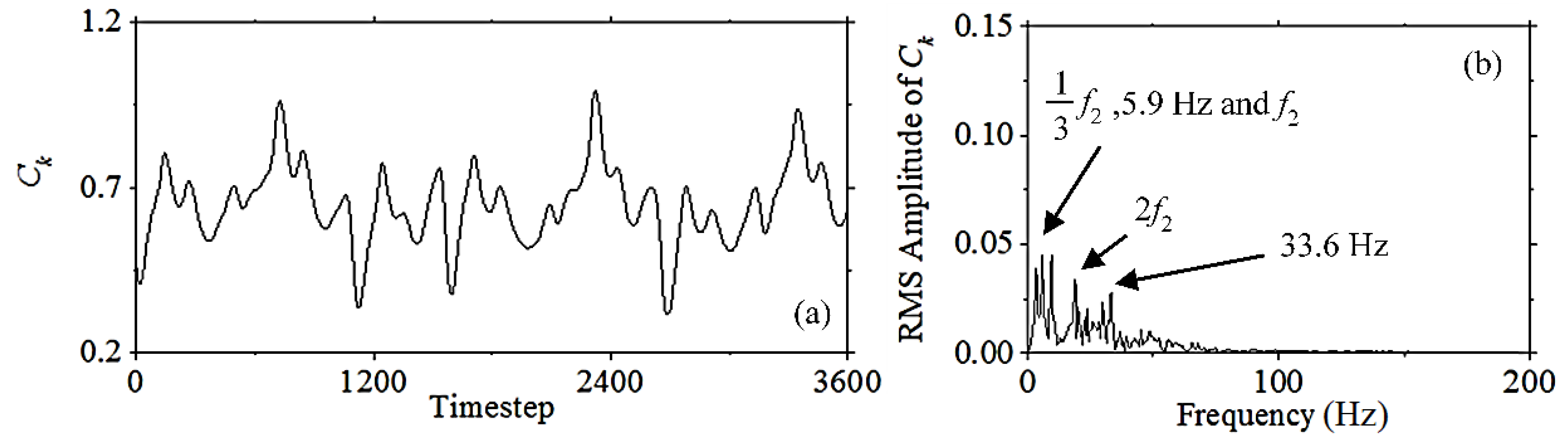
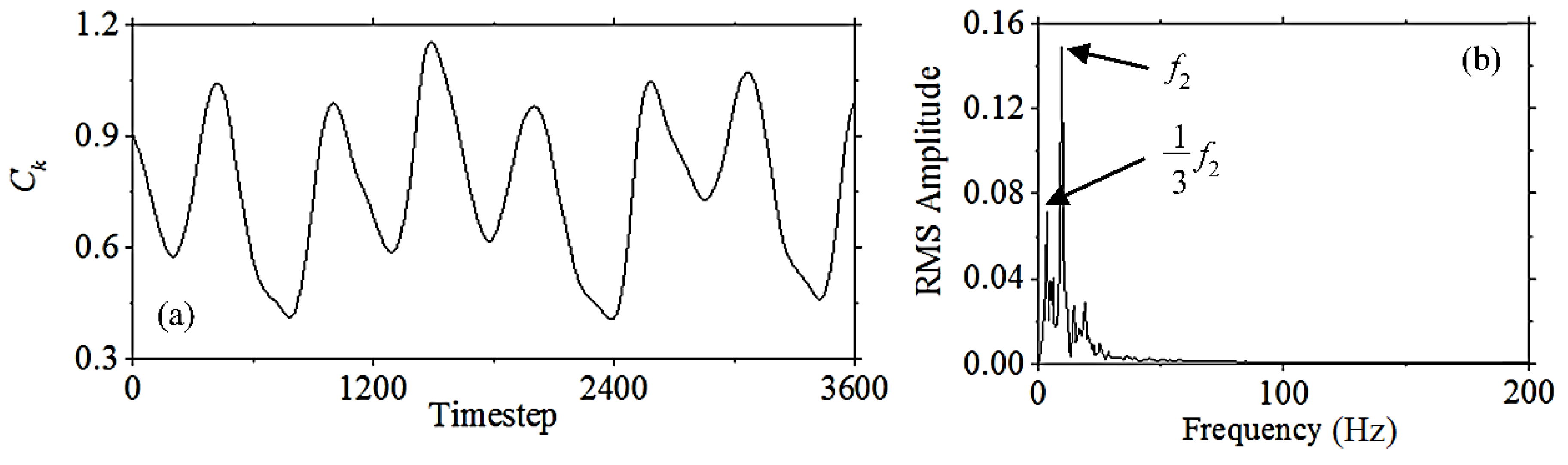
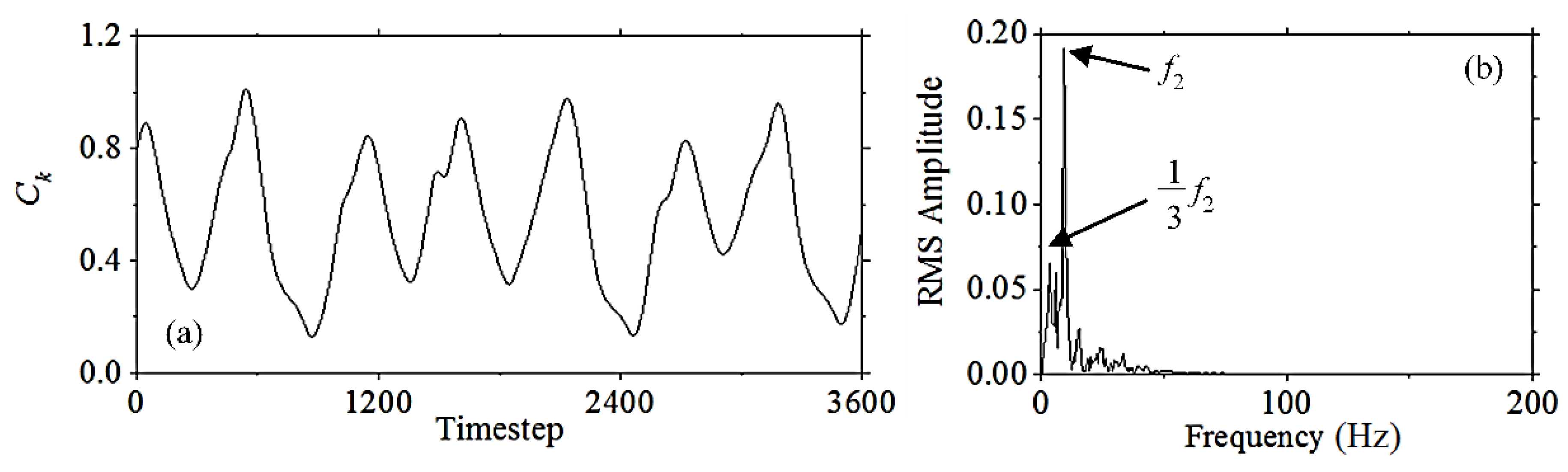
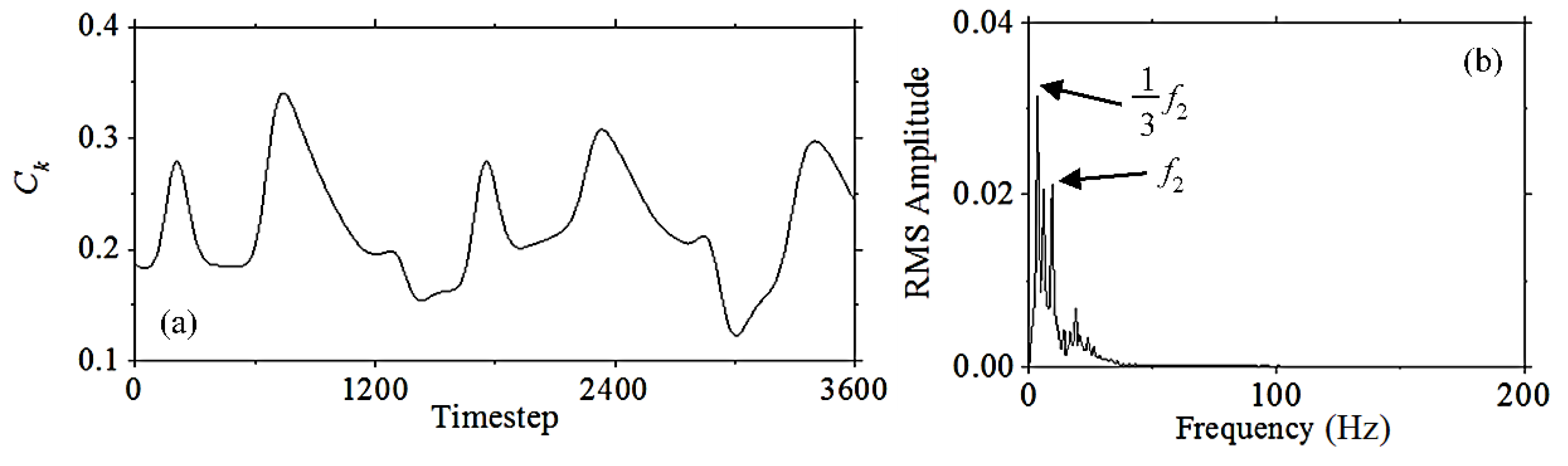
5.4. Turbulence Kinetic Energy Pulsation

To study the pulsation of turbulence kinetic energy, points were set, as shown in Figure 13, for monitoring the C_k variation in the indication regions numbers Ⅰ to Ⅶ. Points P₁ to P₇ are, respectively, in the local flow regions I to Ⅶ. Figure 1, Figure 2, Figure 3, Figure 4, Figure 5, Figure 6, Figure 7, Figure 8, Figure 9, Figure 10, Figure 11, Figure 12, Figure 13, Figure 14, Figure 15, Figure 16, Figure 17, Figure 18, Figure 19 and Figure 20 are the time-domain and frequency-domain plots of C_k on monitoring points P₁ to P₇. The time-domain data were acquired within 3600 timesteps that were five runner revolutions. The frequency-domain data was created based on the time-domain data by applying the fast-Fourier transformation (FFT) method with Hanning window.

The C_k pulsation on P₁ is shown in Figure 14. Multiple peaks can be found on the frequency-domain plot. Some important frequencies can be found including the blade frequency f_b of about 64.5 Hz and another frequency f₂ of about 9.6 Hz. Three peaks are related to the blade frequency f_b are, respectively, f_b, 2f_b, and 3f_b. Three other peaks are related to f₂ are 0.15f₂, f₂, and 3f₂. Generally, P₁ is under the strong influence of blade frequency f_b, which is also a multiple of runner frequency f_rn. This is because P₁ is near the runner blade trailing-edge and faces the incoming flow from runner pumping. The frequency f₂ is also strong and needs further analysis on points P₂ to P₇.

The C_k pulsation on P₂ is shown in Figure 15. The runner blade frequency f_b is still obvious and stronger in amplitude than on P₁. However, the frequency f₂ and its two-times multiple 2f₂ are relatively stronger than f_b. P₂ is in the guide vane jet which is induced by both the runner pumping and the small guide vane opening. Thus, the runner blade frequency impressively influences P₂. Frequency f₂ dominates with the C_k peak value up to about 0.23. Therefore, the f₂-series frequencies on P₁ are propagated from the guide vane jet region.

The C_k pulsation on P₃ is shown in Figure 16. P₃ is in one of the twin-vortexes which rotates in the same direction of runner rotation. The runner blade frequency f_b is no longer strong, but f₂-series dominates. 1/3 f₂, f₂, and 2f₂ are on a high amplitude level. Among them, the C_k amplitude of f₂ is the highest that larger than 0.10. The C_k amplitude of 1/3 f₂ and 2f₂ are also higher than 0.05.

The C_k pulsation on P₄ is shown in Figure 17. P₄ is in another one of the twin-vortexes which rotates counter-rotationally against the runner. Frequency band becomes complex with 1/3 f₂, f₂, 2f₂, and 5.9 Hz and 33.6 Hz peaks. The C_k amplitude of these frequencies are no larger than 0.05 and are lower than that on P₃. This means that the turbulence kinetic energy is lower in the counter-runner-rotational vortex than in the runner-rotational vortex. According to the C_k pulsations on P₃ and P₄, the f₂-series frequencies also exist in the twin-vortexes adjacent to the guide vane jet.

The C_k pulsation on P₅ is shown in Figure 18. The frequency f₂ dominates with the C_k amplitude of about 0.15. The frequency 1/3 f₂ is also strong with the C_k amplitude of about 0.075. The frequency 2f₂ is still on the same C_k amplitude level as on P₂, P₃, and P₄.

The C_k pulsation on P₆ is shown in Figure 19. Both the time-domain and frequency domain are similar to P₅. The C_k amplitude of f₂ increases to about 0.20 on P₆, which is stronger than on P₅. In the stay vane, the influence of runner blade frequency f_b is already very weak and difficult to find on the frequency-domain plots.

The C_k pulsation on P₇ is shown in Figure 20. The frequencies 1/3 f₂ and f₂ are still strong. The C_k amplitude of frequency f₂ is about 0.20, which is similar to that on P₆. However, the C_k amplitude of frequency 1/3 f₂ obviously increases to about 0.03, which is four-times of that on P₆. Both P₆ and P₇ are in the volute, which means that the 1/3 f₂ frequency is the dominate frequency in volute.

Above all, three main C_k pulsation frequencies can be found on P₁ to P₇, as listed in

Table 1. The main frequencies of C_k pulsation on points P₁ to P₇.

Name	Frequency Value	Description
fb	64.5 (Hz)	Runner blade frequency
fgsv	9.6 (Hz)	Dominate frequency in guide vane and stay vane. fgsv = f2
fvl	3.2 (Hz)	Dominate frequency in volute fvl = 1/3 f2

. Firstly, the runner blade frequency f_b dominates in the region near runner blade. Secondly, the frequency f₂ above can be defined as f_gsv because it dominates, mainly in the guide vane and stay vane region. Thirdly, the frequency 1/3 f₂ above can be defined as f_vl because it dominates mainly in volute region.

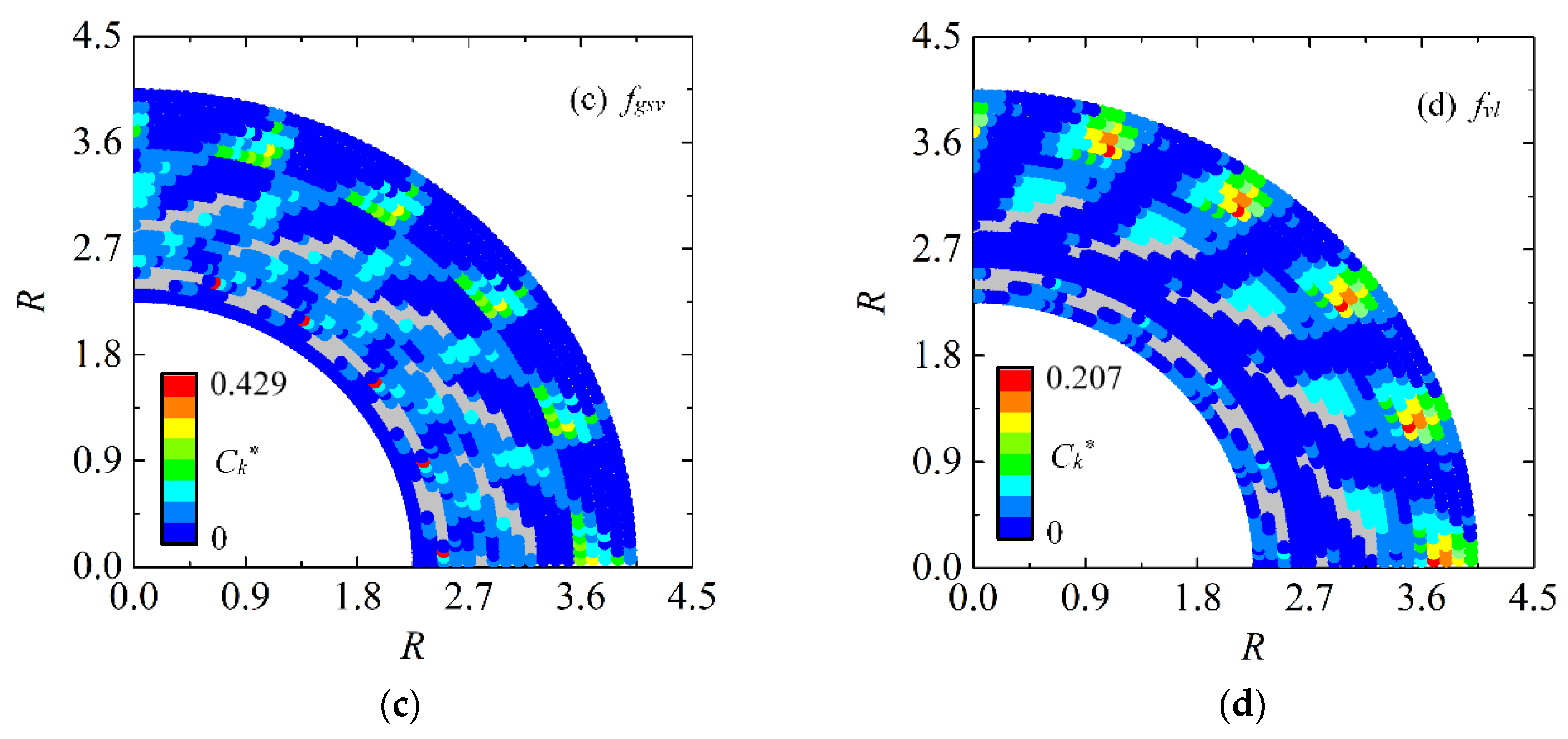
5.5. Propagation of Frequency

To understand the propagation of frequency f_b, f_gsv, and f_vl in the flow passage, the 18 × 18 flow pulsation tracing topology, as shown in Figure 21, is set instead of the points P₁ to P₇. It covers the 1/20 rotational-periodic region including one guide vane passage, one stay vane passage, and a part of the volute passage. Points are ordered as “1~18” along tangential θ direction and as “AA~RR” along radial R direction. Δθ is set as 1 degree, and ΔR is set as 0.1 m. As the same as on P₁ to P₇, the frequencies of C_k are calculated by applying the Fast-Fourier transformation (FFT) method with Hanning window.

In this study, the frequency-dominated turbulence kinetic energy coefficient C_k^* is defined for C_k to understand the propagation of frequency:

$$C_k^{\ast }=\frac{C_{kRMS}}{\Delta C_k}$$

(16)

where C_kRMS is the RMS amplitude value of specific frequency. In this case, the f_b = 64.5 Hz, f_gsv = 9.6 Hz and f_vl = 3.2 Hz are tracked using the topology. ΔC_k is the peak-peak value of C_k within a specific period. Totally, five runner revolutions were studied in this case. Hence, the parameter C_k^* can exclude the amplitude difference of local flow pulsation and focus on the frequency character. Figure 22 shows the contour of C_k^* of f_b = 64.5 Hz, f_gsv = 9.6 Hz, and f_vl = 3.2 Hz. The color from blue to red denotes the amplitude of C_k^*. The blank sites are guide vane blades and stay vane blades. In Figure 22, parameter R is the radial position. Four copies are plotted based on the original 18 × 18 topology to have a better blade-to-blade view in θ = 0~90°.

As shown in Figure 22b, the runner blade frequency f_b mainly affects C_k^* in the region between the runner and guide vane. The highest C_k^* site locates at the front side of the guide vane blade. In the stay vane and volute, the influence of f_b on C_k^* is very weak. According to Figure 22c, the dominate frequency in the guide vane and stay vane f_gsv has a high C_k^* value everywhere in the vane channels. The highest C_k^* value of f_gsv is in the guide vane jet region, which is between two guide vane blades. A wide high C_k^* region can be also found in the volute near the stay vane outlet. Based on Figure 22d, the dominate frequency in volute f_vl has very strong influence on C_k^* in volute. The highest C_k^* sites are between the two stay vane jets and overlap the volute vortex sites. More high C_k^* regions of f_vl are on the back side of the stay vane blade. The region in the guide vane jet is also high in C_k^* under the influence of frequency f_vl.

Generally, the strongly influenced region by f_b = 64.5 Hz, f_gsv = 9.6 Hz, and f_vl = 3.2 Hz can be summarized as follows:

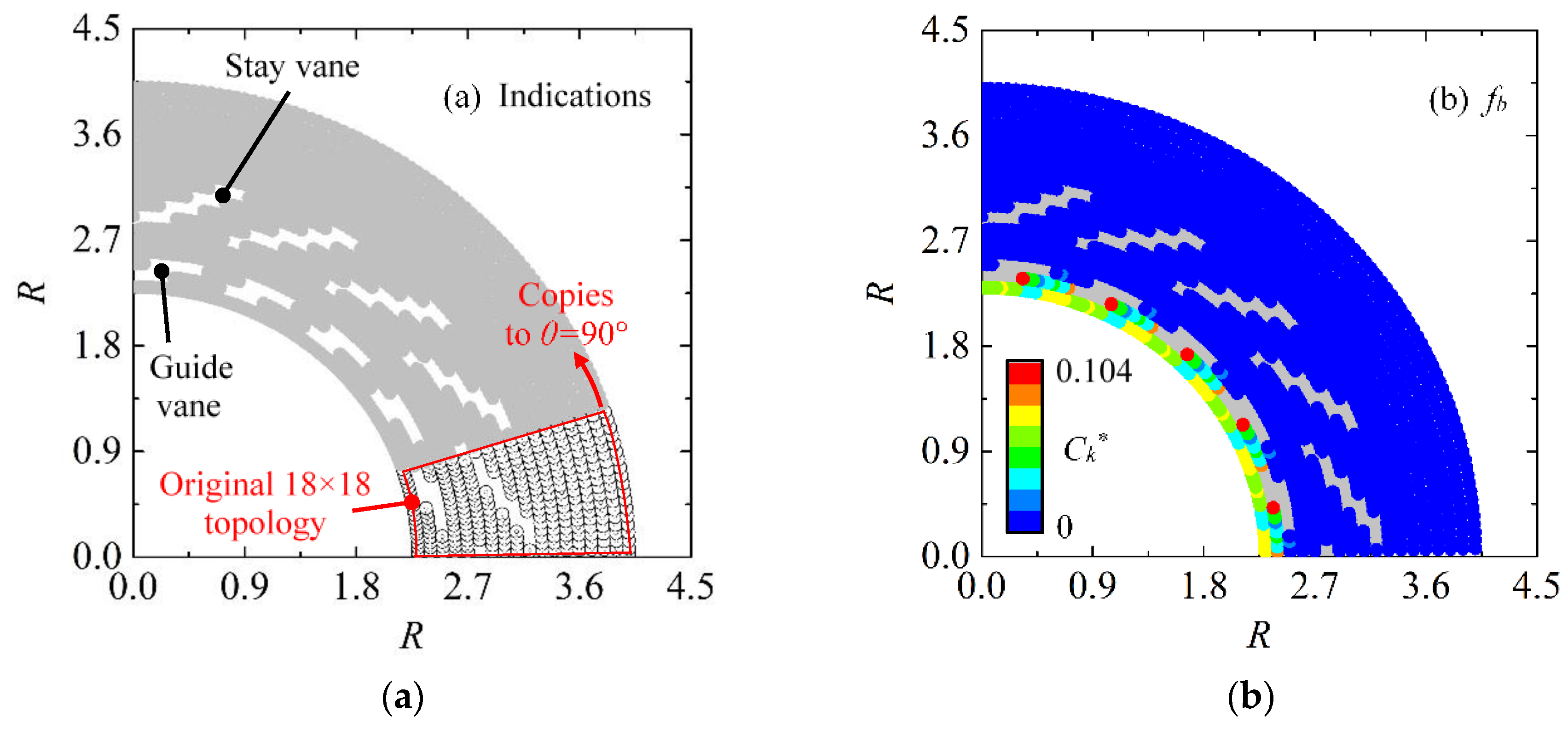
• f_b = 64.5 Hz: (a) Between runner and guide vane; (b) in the guide vane jet;
• f_gsv = 9.6 Hz: (a) In the stay vane and guide vane channels; (b) near volute vortex; (c) in the guide vane jet;
• f_vl = 3.2 Hz: (a) Near volute vortex; (b) on the back side of stay vane blade; (c) in the guide vane jet.

The specific frequencies of flow characteristics are induced by different flow structures. The high amplitude sites of specific frequencies relate to the distribution of flow structures. However, the specific frequencies of turbulent flow may propagate in fluid and influence adjacent regions.

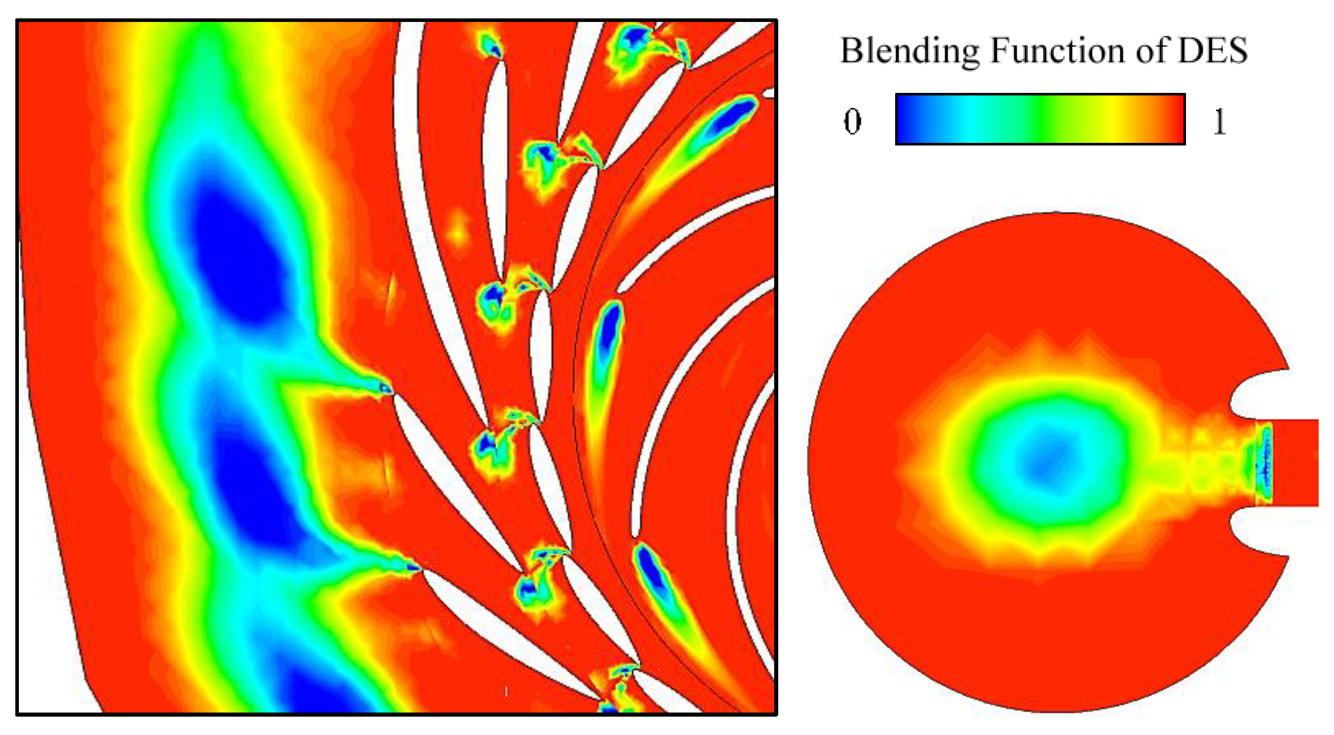
5.6. Checking the Effectiveness of DES

To check the effectiveness of DES, the contour of the DES blending function is plotted in Figure 23. In regions where the DES blending function is 0, the LES model is activated. In the region where the DES blending function is 1, the RANS model is activated. On S_A, it can be seen that the LES model is activated in the runner blade trailing-edge wake, inter guide vane jet, stay vane leading-edge separation region, stay vane trailing-edge wake, and volute vortex. On S_B, the core region in the volute, which is the two symmetrical rotating flow structures’ interaction site, is simulated by the LES model. In these jet and vortex flow regions, the LES model helps to provide a better resolution of turbulent flow. It proves that DES is effective in this study with jet-vortex flow structure from runner outlet to volute.

6. Conclusions

According to the studies above, conclusions can be drawn as follows:

(1)

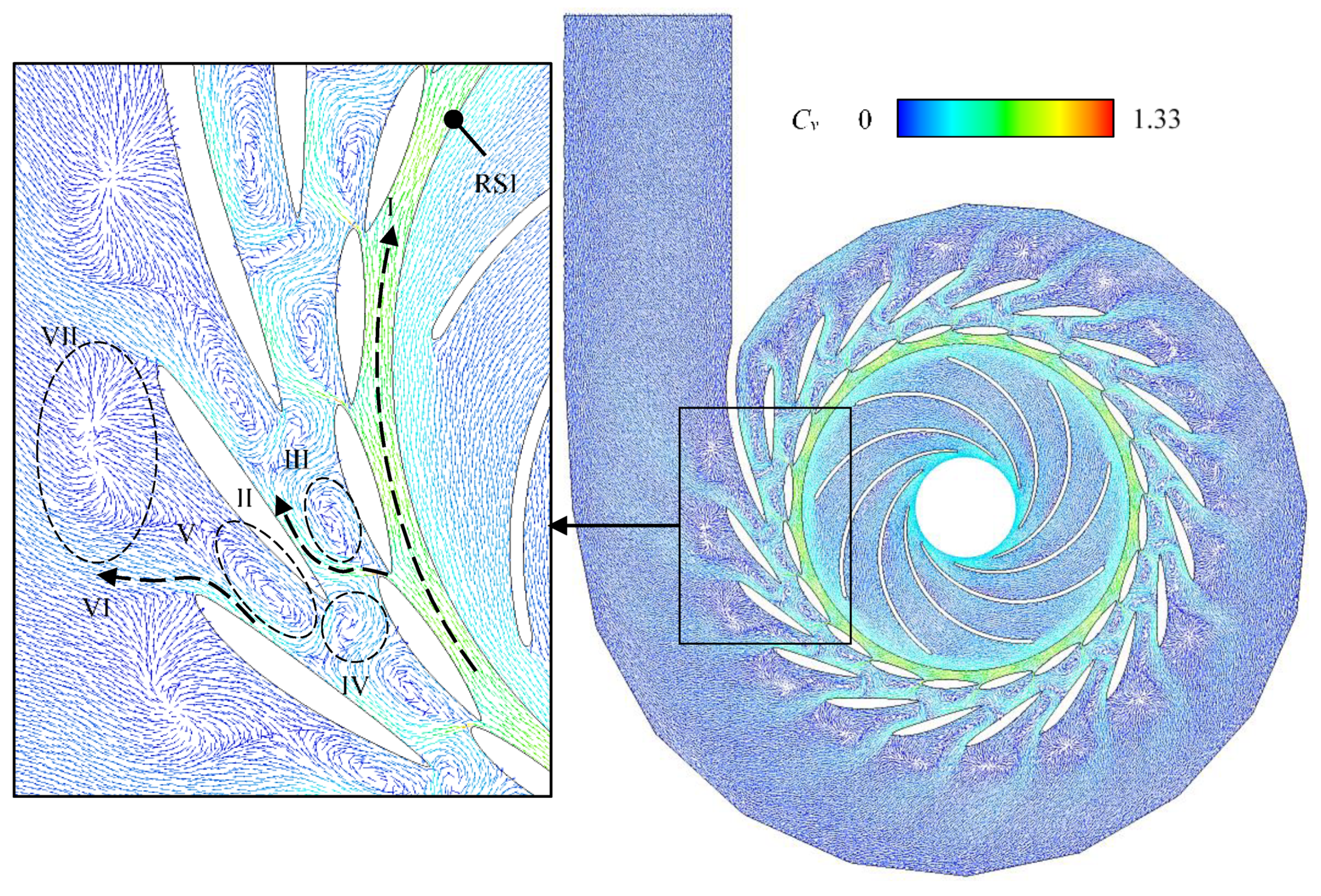
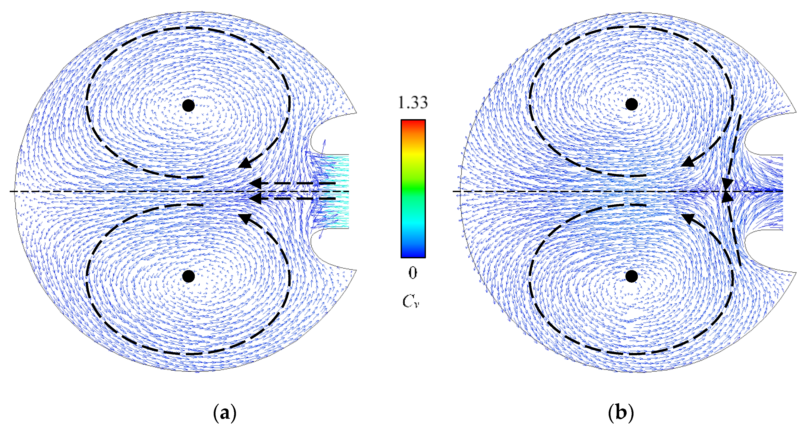
In a pump-turbine’s start-up process in pump mode, flow regime is undesirable due to a small guide vane opening angle. In this study at C_φ = 0.015 and α = 3 degrees, the jet-vortex flow structure can be observed in the diffuser, including the guide vane, stay vane, and volute. It consists of Ⅰ—the flow ring between the runner trailing-edge and the guide vane, Ⅱ—the guide vane jet, Ⅲ and Ⅳ—the twin-vortexes adjacent to guide vane jet, Ⅴ—the inter stay vane vortex, Ⅵ —the stay vane jet, and Ⅶ—the volute vortex-ring. These jets and vortexes interfere with the runner pumping and cause an instability of the flow field.

(2)

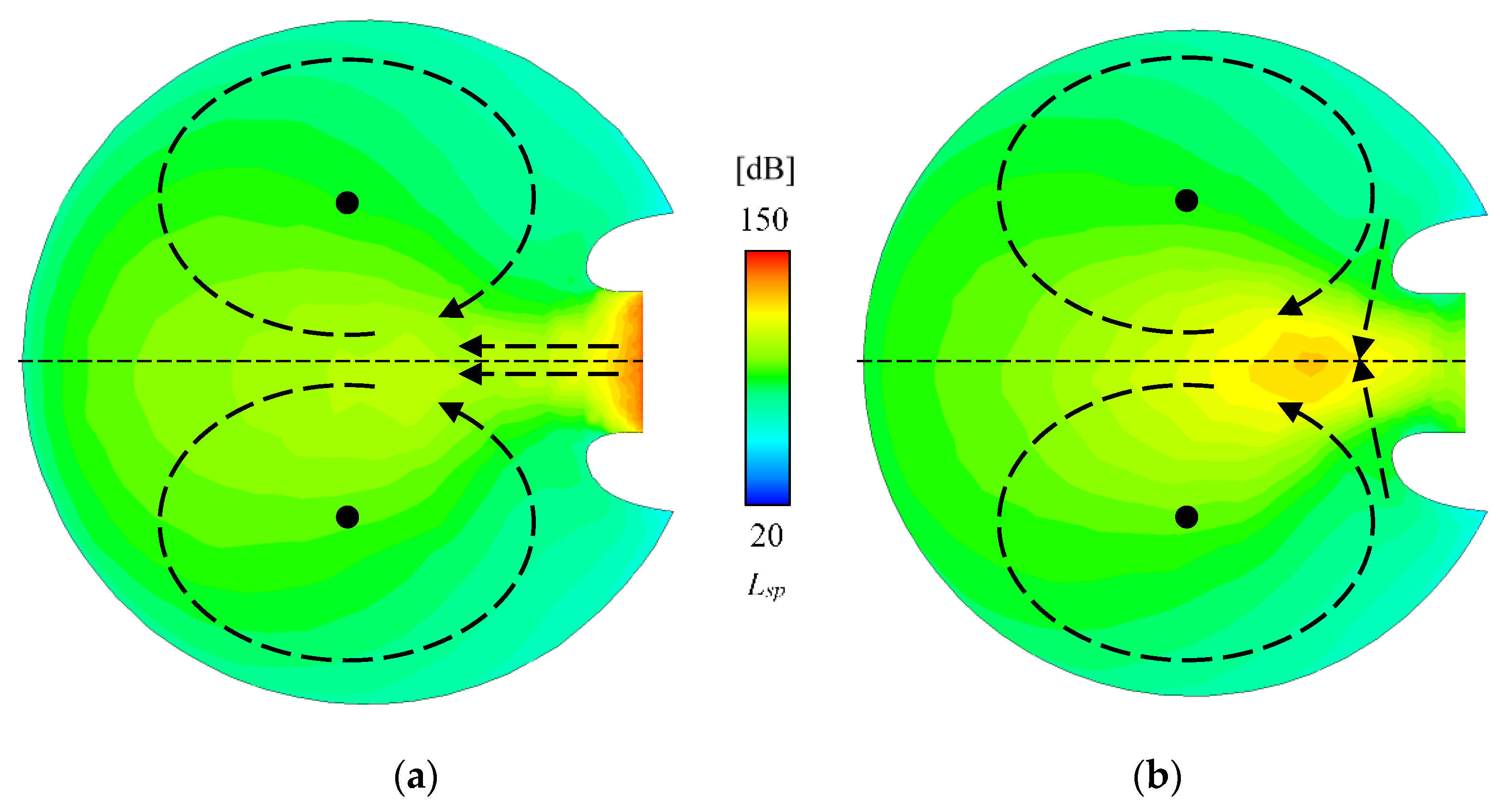
Based on the acoustic analogy method, strong noise can be found in the jet-vortex flow structure. Results show that the high turbulence kinetic energy and eddy dissipation caused by undesirable flow structures could be the reason why noise is generated in the flow passages. High sound power level L_sp regions in the jets and vortexes are caused by high turbulence kinetic energy. High L_sp regions on the blade leading-edges are due to local flow striking and separation with strong eddy dissipation. The strongest L_sp region is in the guide vane jet, where L_sp is up to about 150 dB. This shows that the guide vane opening and direction are the most important factors in inducing noise, especially at small guide vane opening angle conditions.

(3)

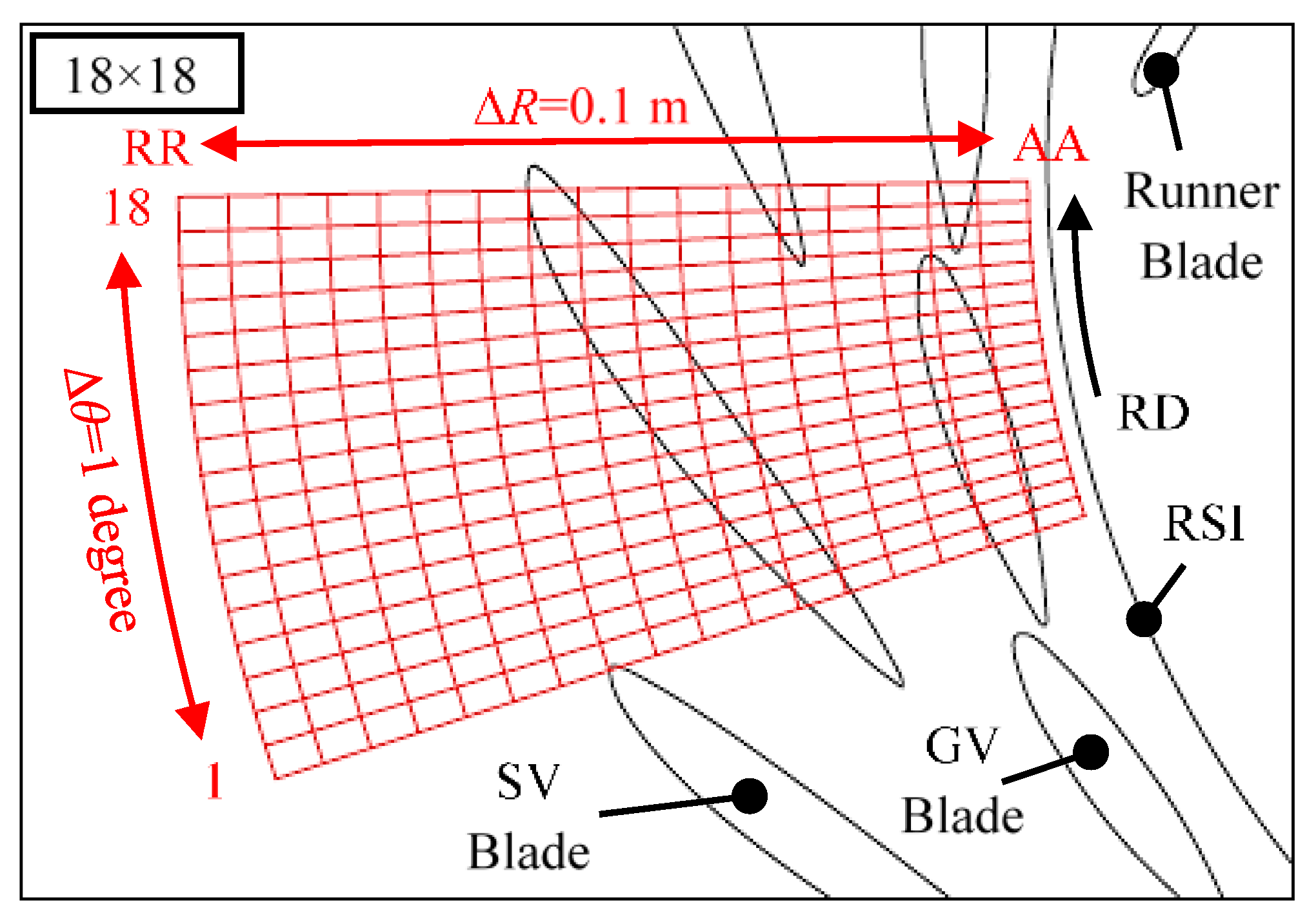
The pulsation of turbulence kinetic energy coefficient C_k was studied on monitoring points P₁ to P₇. Three specific frequencies were found, including the runner blade frequency f_b = 64.5 Hz, the dominate frequency in the guide vane and stay vane f_gsv = 9.6 Hz, and the dominate frequency in the volute f_vl = 3.2 Hz. The 18 × 18 flow pulsation tracing topology gives a better visualization of frequency distribution and propagation. The frequency-dominated turbulence kinetic energy coefficient C_k^* was used instead of C_k to exclude the pulsation amplitude difference. Results show that different specific frequencies are caused by different flow structures. Frequencies will propagate and affect the adjacent regions.

Generally, the guide vane opening angle is found crucial in producing flow noise and turbulence pulsations, especially in the pump mode’s start-up process. A better understanding of the flow regime at the small guide vane opening can help reducing and optimizing the flow noise in the future researches. In this study, the numerical study was done on a prototype scale, but the experimental study was conducted on a model scale. In the future, the tests will be done on a prototype pump-turbine unit to have a better comparative analyses.

References

1. Oishi, A.; Yokoyama, T. Development of high head single and double stage reversible pump-turbines. In Proceedings of the 10th IAHR Symposium on Hydraulic Machinery and Cavitation, Tokyo, Japan, 28 September–2 October 1980. [Google Scholar]
2. Mei, Z. Technology of Pumped-Storage Power Generation; China Machine Press: Beijing, China, 2000. [Google Scholar]
3. Rodriguez, C.G.; Mateosprieto, B.; Egusquiza, E. Monitoring of rotor-stator interaction in pump-turbine using vibrations measured with on-board sensors rotating with shaft. Shock Vib. 2014, 276796. [Google Scholar] [CrossRef]
4. Hasmatuchi, V.; Farhat, M.; Roth, S.; Botero, F.; Avellan, F. Experimental evidence of rotating stall in a pump-turbine at off-design conditions in generating mode. J. Fluids Eng. 2011, 133, 051104. [Google Scholar] [CrossRef]
5. Zhang, Y.; Zhang, Y.; Wu, Y. A review of rotating stall in reversible pump turbine. Proc. Inst. Mech. Eng. Part C J. Mech. Eng. Sci. 2017, 231, 1181–1204. [Google Scholar] [CrossRef]
6. Zuo, Z.; Liu, S.; Sun, Y.; Wu, Y. Pressure fluctuations in the vaneless space of High-head pump-turbines—A review. Renew. Sustain. Energy Rev. 2015, 41, 965–974. [Google Scholar] [CrossRef]
7. Li, Z.; Bi, H.; Karney, B.; Wang, Z.; Yao, Z. Three-dimensional transient simulation of a prototype pump-turbine during normal turbine shutdown. J. Hydraul. Res. 2017, 55, 520–537. [Google Scholar] [CrossRef]
8. Review and outlook of studying on noise of centrifugal pumps. J. Vib. Shock 2011, 30, 77–84.
9. Govern, C.C.; TenWolde, P.R. Energy dissipation and noise correlations in biochemical sensing. Phys. Rev. Lett. 2014, 113, 258102. [Google Scholar] [CrossRef]
10. Bernd, D.; Wurm, F.H. Noise sources in centrifugal pumps. In Proceedings of the 2nd WSEAS International Conference on Applied and Theoretical Mechanics, Venice, Italy, 20–22 November 2006. [Google Scholar]
11. Langthjem, M.A.; Olhoff, N. A numerical study of flow-induced noise in a two-dimensional centrifugal pump. Part II. Hydroacoustics. J. Fluids Struct. 2004, 19, 369–386. [Google Scholar] [CrossRef]
12. Chudina, M. Noise as an indicator of cavitation in a centrifugal pump. Acoust. Phys. 2003, 49, 463–474. [Google Scholar] [CrossRef]
13. Curle, N. The influence of solid boundaries upon aerodynamic sound. Proc. R. Soc. Lond. Ser. A Math. Phys. Sci. 1955, 231, 505–514. [Google Scholar]
14. Ffowcs-Williams, J.E.; Hawkings, D.L. Sound generation by turbulence and surfaces in arbitrary motion. Math. Phys. Sci. 1969, 264, 321–342. [Google Scholar] [CrossRef]
15. Goldstein, J.L. An optimum processor theory for the central formation of the pitch of complex tones. J. Acoust. Soc. Am. 1973, 54, 1496–1516. [Google Scholar] [CrossRef] [PubMed]
16. Lighthill, M.J. On sound generated aerodynamically, II. Turbulence as a source of sound. Proc. R. Soc. Lond. Ser. A 1954, 222, 1–32. [Google Scholar]
17. Chu, S.; Dong, R.; Katz, J. Relationship between unsteady flow, pressure fluctuations, and noise in a centrifugal pump, part B: Effects of blade-tongue interaction. J. Fluids Eng. 1995, 117, 30–35. [Google Scholar] [CrossRef]
18. Srivastav, O.P.; Pandu, K.R.; Gupta, K. Effect of radial gap between impeller and diffuser on vibration and noise in a centrifugal pump. J. Inst. Eng. Mech. Eng. Div. 2003, 84, 36–39. [Google Scholar]
19. Sun, X.; Hu, Z.; Feng, Y.; Zhou, S. An aeroacoustic model about the rotating stall of a compressor. Acta Aeronaut. Astronaut. Sin. 1991, 12, A467–A473. [Google Scholar]
20. Mongeau, L.; Thompson, D.E.; Mclaughlin, D.K. Sound generation by rotating stall in centrifugal turbomachines. J. Sound Vib. 1993, 163, 1–30. [Google Scholar] [CrossRef]
21. Bogey, C.; Marsden, O.; Bailly, C. Large-eddy simulation of the flow and acoustic fields of a Reynolds number 105 subsonic jet with tripped exit boundary layers. Phys. Fluids 2011, 23, 035104. [Google Scholar] [CrossRef]
22. Canepa, E.; Cattanei, A.; Zecchin, F.M.; Milanese, G.; Parodi, D. An experimental investigation on the tip leakage noise in axial-flow fans with rotating shroud. J. Sound Vib. 2016, 375, 115–131. [Google Scholar] [CrossRef]
23. Brooks, T.F.; Hodgson, T.H. Trailing edge noise prediction from measured surface pressures. J. Sound Vib. 1981, 78, 69–117. [Google Scholar] [CrossRef]
24. Wang, W.; Thomas, P.J. Acoustic improvement of stator–rotor interaction with nonuniform trailing edge blowing. Appl. Sci. 2018, 8, 994. [Google Scholar] [CrossRef]
25. Proudman, I. The generation of noise by isotropic turbulence. Proc. R. Soc. Lond. Ser. A Math. Phys. Sci. 1952, 214, 119–132. [Google Scholar]
26. Tao, R.; Zhao, X.; Wang, Z. Evaluating the transient energy dissipation in a centrifugal impeller under rotor-stator interaction. Entropy 2019, 21, 271. [Google Scholar] [CrossRef]
27. Liu, J.; Wang, L.; Liu, S.; Sun, Y.; Wu, Y. Three dimensional flow simulation of load rejection of a prototype pump-turbine. Eng. Comput. 2013, 29, 417–426. [Google Scholar]
28. Nennemann, B.; Parkinson, É. Yixing pump turbine guide vane vibrations: Problem resolution with advanced CFD analysis. IOP Conf. Ser. Earth Environ. Sci. 2010, 12, 012057. [Google Scholar] [CrossRef]
29. Zhu, D.; Xiao, R.; Tao, R.; Liu, W. Impact of guide vane opening angle on the flow stability in a pump-turbine in pump mode. Proc. Inst. Mech. Eng. Part C J. Mech. Eng. Sci. 2017, 231, 2484–2492. [Google Scholar] [CrossRef]
30. Li, D.; Gong, R.; Wang, H.; Han, l.; Wei, X.; Qin, D. Analysis of vorticity dynamics for hump characteristics of a pump turbine model. J. Mech. Sci. Technol. 2016, 30, 3641–3650. [Google Scholar] [CrossRef]
31. Tao, R.; Xiao, R.; Wang, F.; Liu, W. Cavitation behavior study in the pump mode of a reversible pump-turbine. Renew. Energy 2018, 125, 655–667. [Google Scholar] [CrossRef]
32. Gentner, C.; Sallaberger, M.; Widmer, C.; Braun, O.; Staubli, T. Numerical and experimental analysis of instability phenomena in pump turbines. IOP Conf. Ser. Earth Environ. Sci 2012, 15, 032042. [Google Scholar] [CrossRef] [Green Version]
33. Liu, J.; Liu, S.; Wu, Y.; Sun, Y.; Zuo, Z. Prediction of “S” characteristics of a pump-turbine with small opening based on V2F model. Int. J. Mod. Phys. Conf. Ser. 2012, 19, 417–423. [Google Scholar] [CrossRef]
34. Spalart, P.R. Detached-eddy simulation. Annu. Rev. Fluid Mech. 2009, 41, 181–202. [Google Scholar] [CrossRef]
35. Menter, F.R. Two-Equation Eddy-Viscosity Turbulence Models for Engineering Applications. AIAA J. 1994, 32, 1598–1605. [Google Scholar] [CrossRef]
36. Liu, H.; Tan, M. Modern Design Methods for Centrifugal Pumps; China Machine Press: Beijing, China, 2013. [Google Scholar]
37. Celik, I.; Ghia, U.; Roache, P.J.; Freitas, C.J.; Coloman, H.; Raad, P.E. Procedure of estimation and reporting of uncertainty due to discretization in CFD applications. J. Fluids Eng. 2008, 130, 078001. [Google Scholar]
38. Kader, B.A. Temperature and concentration profiles in fully turbulent boundary layers. Int. J. Heat Mass Transf. 1981, 24, 1541–1544. [Google Scholar] [CrossRef]
39. Shankaran, G.; Dogruoz, M.B. Advances in fan modeling—Using multiple reference frame (MRF) approach on blowers. In Proceedings of the ASME 2011 Pacific Rim Technical Conference & Exposition on Packaging and Integration of Electronic and Photonic Systems, Portland, OR, USA, 6–8 July 2011. [Google Scholar]
Figure 1. The schematic map of the pump-turbine in prototype scale shown as a fluid domain.
Applsci 09 01971 g001
Figure 2. The selection and determination of the numerically studied condition based on model test. BEP: best efficiency point. (a) The on-cam relationship between Cφ and Cα based on model test; (b) the model test rig.
Applsci 09 01971 g002
Figure 3. Mesh node number of all the flow components with an enlarged view of the mesh from the runner outlet to the stay vane outlet. DT: Draft tube; RN: Runner; GV: Guide vane; SV: Stay vane; VL: Volute. (a) Mesh node number of all the components; (b) schematic map of mesh.
Applsci 09 01971 g003
Figure 4. Verification for mesh scheme and numerical setup by comparing the Cφ-η data.
Applsci 09 01971 g004
Figure 5. Reference surfaces SA and SB for flow field plotting.
Applsci 09 01971 g005
Figure 6. Flow regime on SA by plotting the Cv vectors. Ⅰ: Flow ring between the runner trailing-edge and the guide vane; Ⅱ: Guide vane jet; Ⅲ and Ⅳ: Twin-vortexes adjacent to guide vane jet; Ⅴ: Inter stay vane vortex; Ⅵ: Stay vane jet; Ⅶ: Volute vortex-ring; RSI: Rotor-stator interface.
Applsci 09 01971 g006
Figure 7. Flow regime on SB in volute at different locations by plotting the Cv vectors. (a) Section across the stay vane jet; (b) section across the volute vortex.
Applsci 09 01971 g007
Figure 8. Instaneous turbulent-flow-induced noise field on SA by plotting the Lsp contour. Ⅰ: Flow ring between the runner trailing-edge and the guide vane; Ⅱ: Guide vane jet; Ⅲ and Ⅳ: Twin-vortexes adjacent to guide vane jet; Ⅴ: Inter stay vane vortex; Ⅵ: Stay vane jet; Ⅶ: Volute vortex-ring; RSI: Rotor-stator interface.
Applsci 09 01971 g008
Figure 9. Instaneous turbulent-flow-induced noise field on SB in volute at different locations by plotting the Lsp contour. (a) Section across the stay vane jet; (b) section across the volute vortex.
Applsci 09 01971 g009
Figure 10. Local high Lsp regions on the blade leading-edges. LE: Leading-edge. (a) Runner leading-edge; (b) Guide vane leading-edge and trailing-edge; (c) Stay vane leading-edge.
Applsci 09 01971 g010
Figure 11. Comparison of Lsp, Ck, and Cε contours. (a) Contour of Lsp; (b) Contour of Ck; (c) Contour of Cε.
Applsci 09 01971 g011
Figure 12. The contour of Cε on the blade leading-edges. LE: Leading-edge. (a) Runner leading-edge; (b) Guide vane leading-edge and trailing-edge; (c) Stay vane leading-edge.
Applsci 09 01971 g012
Figure 13. Points P1 to P7 for monitoring the turbulence flow field. RSI: Rotor-stator interface; RD: Runner rotation direction.
Applsci 09 01971 g013
Figure 14. Analysis of Ck pulsation on P1. (a) Time-domain plot; (b) frequency-domain plot.
Applsci 09 01971 g014
Figure 15. Analysis of Ck pulsation on P2. (a) Time-domain plot; (b) frequency-domain plot.
Applsci 09 01971 g015
Figure 16. Analysis of Ck pulsation on P3. (a) Time-domain plot; (b) frequency-domain plot.
Applsci 09 01971 g016
Figure 17. Analysis of Ck pulsation on P4. (a) Time-domain plot; (b) frequency-domain plot.
Applsci 09 01971 g017
Figure 18. Analysis of Ck pulsation on P5. (a) Time-domain plot; (b) frequency-domain plot.
Applsci 09 01971 g018
Figure 19. Analysis of Ck pulsation on P6. (a) Time-domain plot; (b) frequency-domain plot.
Applsci 09 01971 g019
Figure 20. Analysis of Ck pulsation on P7. (a) Time-domain plot; (b) frequency-domain plot.
Applsci 09 01971 g020
Figure 21. The 18 × 18 topology for tracing the frequency propagation. RSI: Rotor-stator interface; RD: Runner rotation direction; GV: Guide vane; SV: Stay vane; 1~18: Order number along tangential direction; AA~RR: Order number along radial direction.
Applsci 09 01971 g021
Figure 22. Contour of Ck* of fb = 64.5 Hz, fgsv = 9.6 Hz and fvl = 3.2 Hz. (a) Indications; (b) Contour of fb; (c) Contour of fgsv; (d) Contour of fvl.
Applsci 09 01971 g022aApplsci 09 01971 g022b
Figure 23. Checking the blending function of the Detached Eddy Simulation (DES) on SA and in the specific region on SB.
Applsci 09 01971 g023