GPU Acceleration of Hydraulic Transient Simulations of Large-Scale Water Supply Systems

Abstract

Simulating hydraulic transients in ultra-long water (oil, gas) transmission or large-scale distribution systems are time-consuming, and exploring ways to improve the simulation efficiency is an essential research direction. The parallel implementation of the method of characteristics (MOC) on graphics processing unit (GPU) chips is a promising approach for accelerating the simulations, because GPU has a great parallelization ability for massive but simple computations, and the explicit and local features of MOC meet the features of GPU quite well. In this paper, we propose and verify a GPU implementation of MOC on a single chip for more efficient simulations of hydraulic transients. Details of GPU-MOC parallel strategies are introduced, and the accuracy and efficiency of the proposed method are verified by simulating the benchmark single pipe water hammer problem. The transient processes of a large scale water distribution system and a long-distance water transmission system are simulated to investigate the computing capability of the proposed method. The results show that GPU-MOC method can achieve significant performance gains, and the speedup ratios are up to hundreds compared to the traditional method. This preliminary work demonstrates that GPU-MOC parallel computing has great prospects in practical applications with large computing load.

1. Introduction

Hydraulic transients are the fluctuations of pressure and flow in water (oil, gas) transmission or distribution systems caused by pump or valve operations, and their numerical simulations are essential for design, operation and management of engineering projects [1,2,3]. The existing simulation methods of hydraulic transients are adequate for many practical applications in terms of accuracy and efficiency [4]. But in some special cases, simulation efficiency must be improved to better meet demands. First, more and more water transmission systems longer than hundreds of kilometers (e.g., the Da Huofang project and the Liaoning northwest water supply project in China are 354 kilometers and 598.4 kilometers, respectively) and water distribution networks containing thousands of pipes, loops, and branches (e.g., the networks in Xiongan New Capital City and Wuhan New Yangtze River City, China) are newly built and planned, for which the hydraulic transient simulations are very time-consuming, normally needing several hours for calculating one working condition. Second, some of these long-distance systems are equipped with real-time monitoring and need online transient simulations for instant decision-making on operations, for which the existing methods are not competent [5]. Third, in design and optimization of many complex pipe systems, a large number of layouts and working conditions should be simulated in a limited time [6]. Therefore, it is necessary to find more efficient simulation methods of hydraulic transients.

Two approaches on improving the computing efficiency of hydraulic transients have already been done. The first is to adopt more efficient algorithms. Wood et al. [7,8] proposed the wave characteristic method (WCM) to efficiently simulate the transient processes of water distribution systems. Boulos et al. [9] and Jung et al. [10] further proved WCM is more efficient than the widely-used method of characteristics (MOC) because of its larger time-step interval and exemption from interior section computation. The second approach is to optimize or parallelize computing codes. Izquierdo and Iglesias [11,12] established a sub-procedure library for general hydraulic boundaries, which were invoked directly in simulations to avoid tiny segmentation and reduce resource occupancy. Li et al. [13] used a parallel genetic algorithm (PGA) in the transient simulations with cavitation and obtained about 10 times of speedup compared to the serial genetic algorithm. Martinez et al. [14] used an optimized genetic algorithm to redesign existing water distribution networks that do not operate properly. Fan et al. [15] parallelized two computers to simulate the transients of several large hydraulic systems, and achieved an efficiency of 1.442 times to that on a single computer. However, these efficiency improvement are far from meeting the practical needs, therefore, new approaches should be explored.

The graphic processing unit (GPU) has shown powerful capability in non-graphical computations and scientists have started using it to conduct large-scale scientific calculations at the beginning of the 21 century [16]. Many successful GPU applications in fluid dynamics calculations have shown quite promising performance gains. Wu et al. [17] accelerated the simulations of fluid structure interaction (FSI) by implementing the immersed boundary-lattice Boltzmann coupling scheme on a single GPU chip, and the attained memory efficiencies for the kernels were up to 61%, 68%, and 66% for the testing case. Bonelli et al. [18] accelerated the simulations of high-enthalpy flows by implementing the state-to-state approach on a single GPU chip, the comparison between GPU and CPU showed a speedup ratio up to 156, and such speedup ratio increased with the problem size and the problem complexity. Zhang et al. [19] implemented a multiple-relaxation-time lattice Boltzmann model (MRT-LBM) on single GPU, and found the GPU-implemented MRT-LBM on a fine mesh can efficiently simulate two-dimensional shallow water flows. Griebel et al. [20] simulated three-dimensional multiphase flows on multiple GPUs of a distributed memory cluster, and the achieved speedup ratios on eight GPUs were 115.8 and 53.7 compared to a single CPU. The supercomputing power of GPU comes from its thousands of cores [21], for example, the number of cores for the latest single GPU GTX Titan Z is up to 5760, and the core number of GPU will continue to grow as the technology develops. Therefore, GPUs show a broad prospect in accelerating computations.

Unfortunately, the use of GPUs is sometimes hampered by the fact that most of the scientific codes written in the past should be ported to GPU architecture. Efforts on this should be done; an important example is the porting of a sophisticated CFD code for compressible flows, originally developed in Fortran and described in [22]. Implementing MOC on GPUs is also an effort on this kind of work. By analyzing the explicit and local characteristics of MOC, we find MOC has a good data independence which is very suitable to be implemented on GPU architectures [23]. To our knowledge, there is no existing report about parallelizing MOC computations on GPUs to accelerate hydraulic transient simulations.

In this paper, we propose and verify a GPU implementation of MOC (GPU-MOC), and try to apply it to transient simulations of practical systems.

2. Implementation of GPU-MOC Method

The essence of GPU acceleration is that it allows thousands of threads to execute in parallel. To be specific, a GPU graphics card is made up of a series of streaming multiprocessors (SM), and it allows thousands of threads to be executed at the same time [24]. Taking the TITAN X chip for example, it is composed of 24 SMs, and in each SM can reside 2048 threads at most. Therefore, a single GPU card can run 49,152 threads in total, at most, at the same time.

2.1. Characteristics of a GPU

A distinguishing feature of a GPU is that the greater number of threads that it includes, the higher efficiency that it can achieve. The reasons may be ascribed to the structure and instruction load of Compute Unified Device Architecture (CUDA). Thread switching is a zero-cost fine-grained execution on a GPU. That is, when a warp (the basic execution unit) in one block has to wait for access to off-chip memory or synchronizing instructions, a warp in another block in a ready state instead will execute the calculation immediately. In this way, computational latency is efficiently hidden and a high throughput is achieved.

2.2. Parallel Characteristics of MOC

The basic equations for unsteady flow are a pairs of hyperbolic partial differential equations as follows.

Continuity equation:

$$A\frac{\partial H}{\partial t}+\frac{a^2}{g}\frac{\partial Q}{\partial x}=0$$

(1)

Momentum equation:

$$\frac{\partial Q}{\partial t}+gA\frac{\partial H}{\partial x}+\frac{fQ\left|Q\right|}{2DA}=0$$

(2)

where H(x,t) is piezometric head; Q(x,t) is discharge; D, A, a, g, and f are the diameter, cross-section area of the pipe, wave speed, acceleration of gravity, and the Darcy-Weisbach friction factor, respectively.

The continuity and momentum equations are transformed into two pairs of equations which are grouped and identified as C⁺ and C⁻, Equations (3) and (4), by the method of characteristics [25], and the final formulas can be expressed as Equations (5) and (6):

$$C^{+}:\{\begin{array}{l}\frac{dH}{dt}+\frac{a}{gA}\frac{dQ}{dt}+\frac{a}{g}\frac{fQ\left|Q\right|}{2D{A}^2}\\ \frac{dx}{dt}=+a\end{array}$$

(3)

$$C^{-}:\{\begin{array}{l}-\frac{dH}{dt}+\frac{a}{gA}\frac{dQ}{dt}+\frac{a}{g}\frac{fQ\left|Q\right|}{2D{A}^2}\\ \frac{dx}{dt}=-a\end{array}$$

(4)

$$Q_P=\frac{C_n-C_m}{B_n+B_m}$$

(5)

$$H_P=\frac{C_n{B}_m+C_m{B}_n}{B_n+B_m}$$

(6)

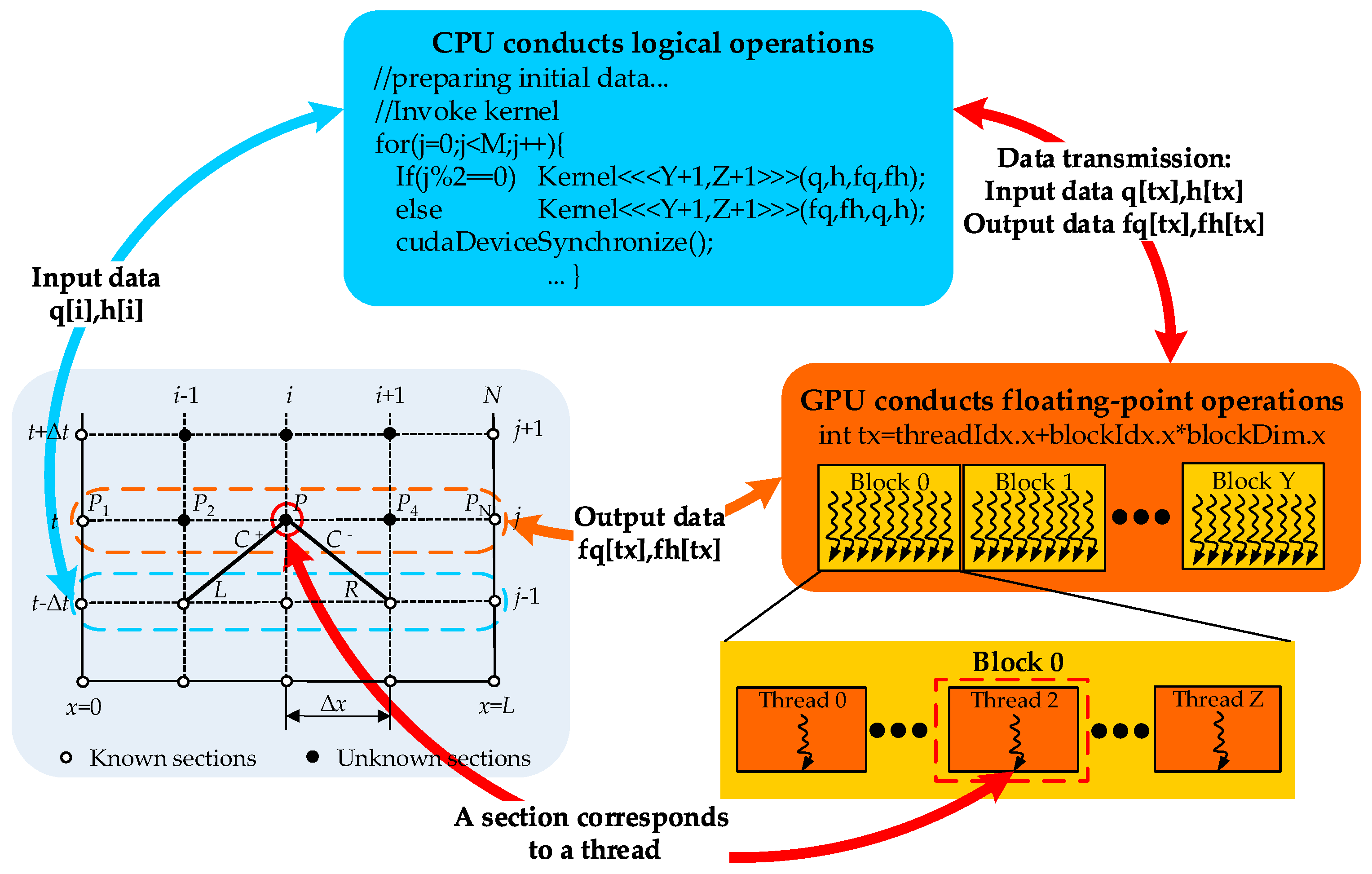
where Q_L, Q_R, Q_P H_L, H_R, and H_P are the discharge and head of sections L, R, and P, in which discharge and head of sections L and R are known; the coefficients $C_n=H_L+B{Q}_L$, $B_n=B+R\left|Q_L\right|$, $C_m=H_R-B{Q}_R$, $B_m=B+R\left|Q_R\right|$, $R=f\Delta x/(2gD{A}^2)$, and $B=a/(gA)$ are known constants; $\Delta x$ is the space interval. As shown in the Cartesian mesh in the x-t plane (Figure 1), through Equations (5) and (6), the values of section P can be calculated by those of sections L and R. The values of other sections at the same time level as P can be solved with the same process.

The solution process described above reflects the explicit and local features of MOC, which is the most critical point for parallelizing MOC on GPU. The explicit feature refers to that the values at section P at the unknown time level is only related to the values at section L and R at the previous time level, having nothing to do with the values at other sections P_i at the same time level as P. The local feature refers to that the values of each section are just connected with the values of its adjacent sections. These features match the multi-thread parallel characteristics of GPU quite well. Therefore, MOC can be built conveniently on a GPU-based CUDA architecture platform, which may fully take advantage of GPU (strong ability of floating-point computing) to compensate the drawbacks of MOC.

2.3. Implementation of MOC on a GPU

The basic GPU-MOC parallel strategy is that the logical operations are conducted on a CPU and the floating-point operations are executed on a GPU. The logical operations like initializing data, allocating memory for arrays, transferring data between the host and device, and invoking MOC kernels, are executed on the CPU, because the CPU has many logical processing units and is efficient in disposing complex logical operations. The floating-point operations, including calculating the present time level values and updating them to the previous time level values, are conducted on GPU, because GPU is equipped with the layouts of pipelines and is efficient in disposing simple floating-point operations.

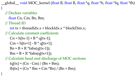
2.3.1. MOC Kernel on GPU

The MOC kernel, executed on GPU, mainly calculates value of all MOC sections. The execution configuration and parameters for MOC kernel are outlined in Figure 1, in which the thread blocks and the thread grid are organized as 1D linear form that fits the line structure of pipeline well. The thread grid includes Y+1 thread blocks, and each thread block contains Z+1 threads. Each thread is allocated to a MOC section, thus, the total number of threads is equal to the total number of MOC sections. During the calculation, threads are located by thread index tx, which is accessible within the kernel through the built-in threadIdx.x and blockIdx.x variables. Threads that indexed in consecutive can be accessed by global memory at the same time to calculate the corresponding MOC sections. The problem of non-aligned access is unnoticeable because the information of the adjacent MOC sections like L and R are in linear order. Thus, shared memory may not make obvious improvement in computing efficiency. In Appendix A, an example of the MOC kernel for direct water hammer is given.

When deciding the threading arrangement, great care should be taken in terms of the block size (number of threads per block), which may affect computing efficiency in some degree. Since resources of shared memory and registers for each block are limited, and number of threads per block and number of blocks per SM are limited. Too large or too small of a block size may reduce the number of threads in each SM. Therefore, reasonable allocation of the block size is important to achieve a high computing efficiency.

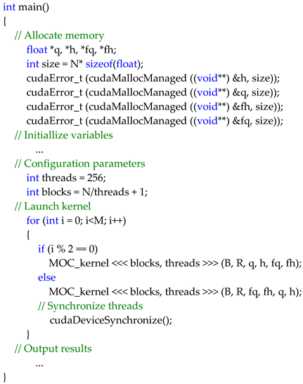
2.3.2. Implementation Procedures on CPU

GPUs and CPUs maintain their own dynamic random access memory (DRAM). Data transmission between GPU memory and CPU memory is the bridge between GPU and CPU. In order to simplify the codes on CPU, the unified memory is adopted. The codes of data transmission between CPU memory and GPU memory are omitted, because unified memory can access both CPU memory and GPU memory. Though codes for data transmission process are omitted, it is still needed to be conducted. Thus, the computing efficiency is not improved.

Data transmission process usually includes three steps: first, copy input data from the CPU memory to the GPU memory; second, load the GPU codes and execute them; and, thirdly, copy output results from the GPU memory back to CPU memory. It is worth mentioning that data transmission efficiency is the determining factor that limits the computational efficiency of the GPU, and many optimizing strategies are aimed at accelerating these processes or reducing data transfer loads.

Two sets of 1D arrays are used to store discharge and head variables for MOC sections, one stores input data and the other stores output data. Initially, the input data are stored in arrays q[tx] and h[tx], and the output data will be stored in arrays fq[tx] and fh[tx]. After the calculation of one time step, the output data are used as the input data for the next time step. Then the input data are stored in fq[tx] and fh[tx], and the output data have to be stored in q[tx] and h[tx] instead. As a result, the MOC kernel has to be invoked alternately by parity counts to switch the arrays that store input and output data. A synchronous function cudaDeviceSynchronize() is used to make sure all computation of this time step are completed before starting the next time step calculation.

In general, the implementation procedures of the CPU codes are listed as follows.

(1)

Allocate unified memory and initialize two set of arrays, and copy input data from the CPU memory to the GPU memory.

(2)

Launch MOC kernel for parallel computing.

(3)

Synchronize threads.

(4)

Write the output data back from the GPU memory to the CPU memory, and set them as input data for the next time step.

(5)

Repeat steps (2)–(4) until the calculation for the last time step finishes.

(6)

Output the results.

In Appendix B, the details of the CPU codes for direct water hammer are given.

3. Verification of GPU-MOC by Benchmark Cases

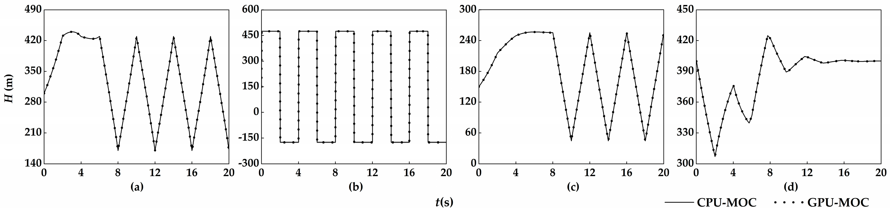
The benchmark cases regarding water hammer in a simple reservoir-single pipe-valve system are simulated to verify the performance of GPU-MOC. The water level of reservoir is constant, and the hydraulic transients are caused by the operations of the end valve. Four benchmark water hammer phenomena, including direct water hammer, first-phase water hammer, last-phase water hammer, and negative water hammer, are simulated. The CPU-MOC program is compiled by the standard C based on Visual Studio 2010 and the GPU-MOC program is compiled by the combination of standard C and CUDA C (an extended language of standard C) based on Microsoft Visual Studio 2010 (Microsoft Corporation: Redmond, WA, USA) and NVIDIA CUDA 8.0 (Nvidia Corporation: Santa Clara, CA, USA).

The results of GPU-MOC and CPU-MOC show quite minor difference and agree well with the pressure variation laws of the four water hammer phenomena (Figure 2), which successfully prove the correctness of the proposed method.

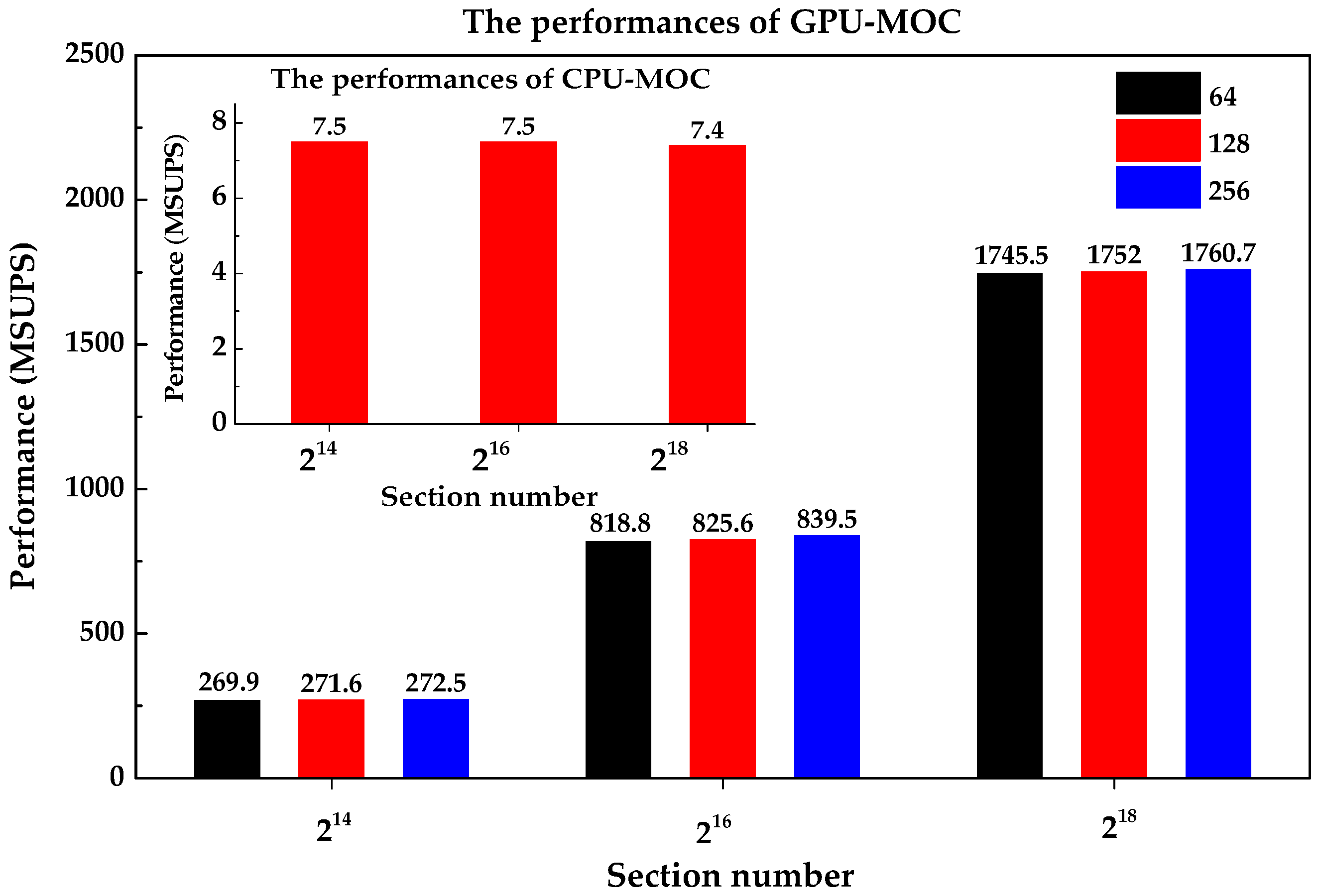
Here, the computing efficiency of direct water hammer simulation is analyzed. Since the efficiency of GPU-MOC strategy is only sensitive to the number of calculations, it is assumed that the pipe length is long enough to be partitioned into sufficient calculation sections. Three cases are simulated, in which the total section numbers are 2¹⁴, 2¹⁶, and 2¹⁸, respectively. Three scenarios of block size (number of threads per block) 64, 128, and 256 are included in each case for GPU-MOC method to find out the effect of block size on computing efficiency. The transient behavior of 20 s is simulated by using single precision. All the calculations are conducted on the computer that is configured with one CPU processor (Intel Xeon e5-2620 v3 2.4G 12 cores, Intel Corporation: Santa Clara, CA, USA) and one graphics card (NVIDIA Geforce GTX TITAN X, Nvidia Corporation: Santa Clara, CA, USA), and the testing platform is Windows 10 64-bit operating system (Microsoft Corporation: Redmond, WA, USA). Moreover, all the simulations are run for at least several times to avoid the effect of machine temperature variation and possible frequency down-stepping of the GPU. Each simulation starts when the GPU is cooled down to room temperature.

The performances of GPU-MOC are much better than those of CPU-MOC. As shown in Figure 3, the maximum performance for GPU-MOC is up to 1760.7 MSUPS (millions of section updates per second), while for CPU-MOC is only 7.5 MSUPS. The reason is that the GPU executes in parallel while the CPU executes serially. Note that the performance data are given in millions of section updates per second (MSUPS). Moreover, the performances of GPU-MOC improve as the section numbers increase. This is because sufficient active warps in the chip can effectively hide the computational latency and achieve a high throughout.

The same trend can be found in

Table 1. Speedup ratios of GPU-MOC to CPU-MOC.

Section Numbers	GPU-MOC with Different Block Sizes
	64	128	256
214	36	36.2	36.3
216	109.2	110.1	111.9
218	234.6	235.5	236.6

, in which the speedup ratios (the ratios of updating section numbers per second of GPU-MOC to those of CPU-MOC) increase as the section numbers increase, ranging from 36 to 236.6 when the section numbers increase from 2¹⁴ to 2¹⁸. Moreover, for each case, GPU-MOC can achieve its best performance when the block size is 256. This is because a block size of 256 just makes a full use of the device processing capacity. Therefore, the block size of 256 is adopted in the following application cases.

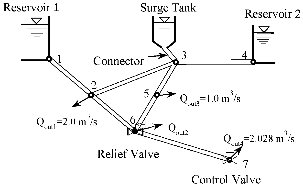
4. Application of GPU-MOC to a Water Distribution Network System

The transient process of an actual water distribution network system (Figure 4) in Karney’s work [26] is simulated. The length of the original system (

Table 2. The length of pipe for different Cases.

Pipe Number	L1 (1 to 2)	L2 (2 to 3)	L3 (3 to 4)	L4 (3 to 5)	L5 (6 to 5)	L6 (2 to 6)	L7 (6 to 7)
Case 1	1001.2	2000	2000	502.5	502.5	1001.2	2000.2
Case 2	10,012	20,000	20,000	5025	5025	10,012	20,002
Case 3	100,120	200,000	200,000	50,250	50,250	100,120	200,020

), namely Case 1, is about 9 km, with seven nodes along the pipeline, a surge tank at node 3, a relief valve at node 6, and a control valve at node 7 (partially closed with $\tau$ = 0.6 initially). The transient phenomena are caused by closing the control valve from opening $\tau$ = 0.6 to $\tau$ = 0.2 within 10 s. The relief valve is initially closed, but it is set to open linearly within 3 s once the pressure exceeds 210 m and then it is closed linearly within 60 s. Details of other parameters can be found in [26].

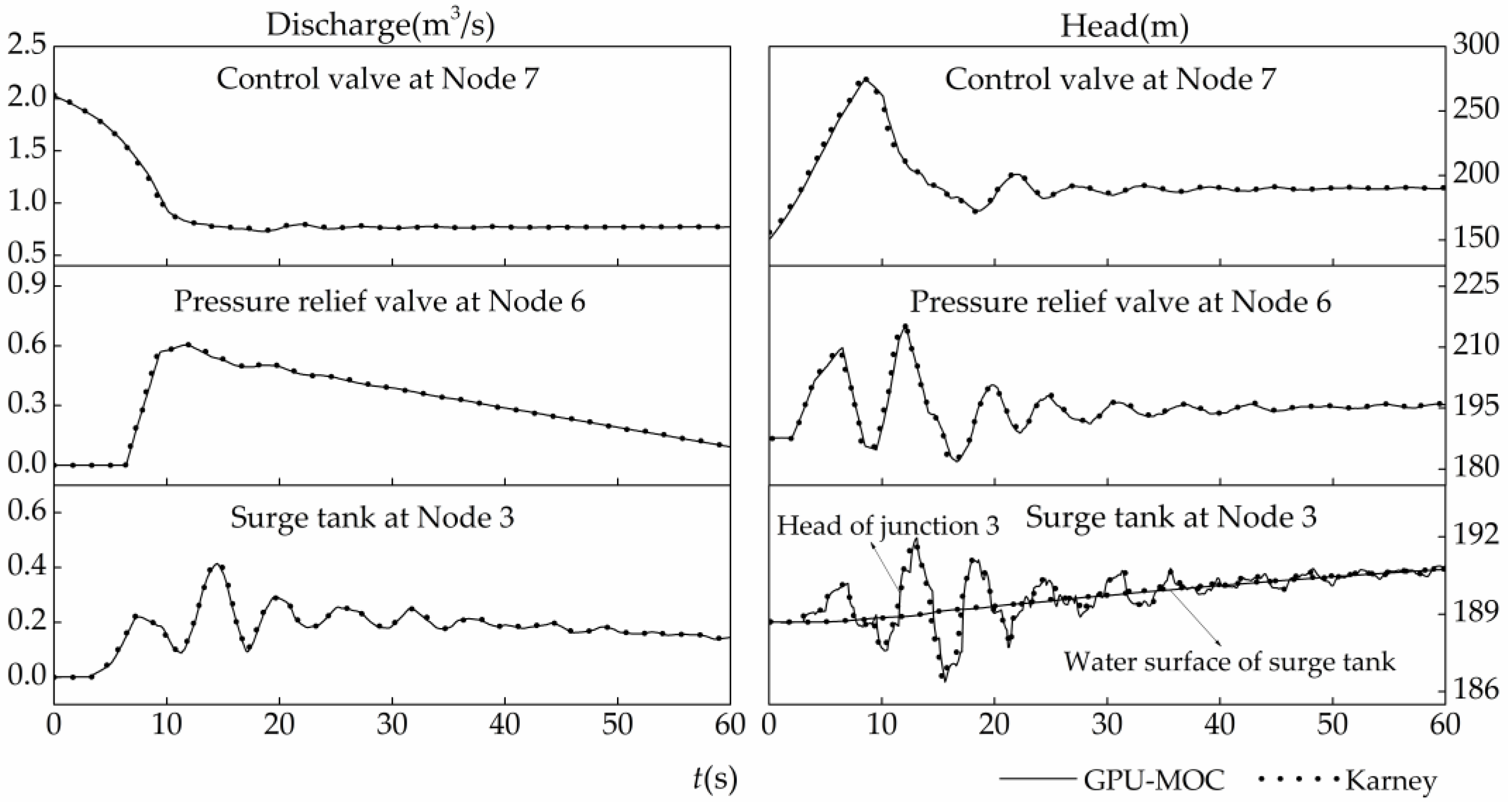
As shown in Figure 5, the results of GPU-MOC and Karney’s work at nodes 3, 6, and 7 show quite minor differences. Thus, the GPU-MOC method is reliable. The high pressure waves initiated at node 7 by the closing valve are propagated throughout the system. At t = 3 s water starts to flow into the surge tank and makes the tank water level rises gradually, and pressure at junction 3 fluctuates in a relative narrow range. The pressure relief valve exceeds 210 m at t = 6.4 s. When the valve opens, the release of fluid at that location reduces the pressure. The water through the relief valve at node 6 and the water level change in the surge tank at node 3 attenuate the transient pressure and allow the system to reach steady state quickly.

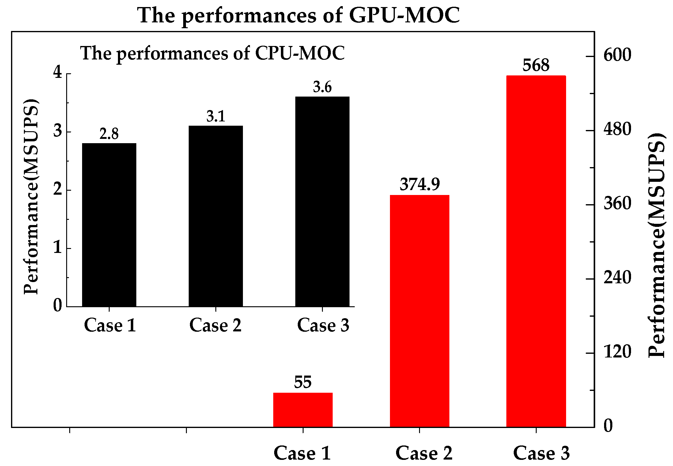
To demonstrate the strong computing capability of the GPU-MOC in computing intensive problems, the pipe length of the above Case 1 is increased tenfold and hundredfold, which are corresponding to Case 2 and Case 3 (Table 2), respectively. The pipe segment lengths $\Delta x$ of Case 1, Case 2 and Case 3 are all set to 1 m, and the corresponding section numbers are 9014, 90,077, 900,767, respectively. The first 60 s transient behavior of the system caused by operating the control valve at node 7 is simulated. The block size is set to 256.

The performances of GPU-MOC are much better than those of the CPU-MOC (Figure 6). The maximum performance for GPU-MOC is up to 568 MSUPS, but for CPU-MOC is only 3.6 MSUPS. In addition, the performances of GPU-MOC improve significantly as the scale of the system becomes larger. For Case 3, it updates 568 MSUPS, but for Case 1 is only 55 MSUPS. That is to say, the computing efficiency of Case 3 is more than 10 times to that of Case 1.

The consumed time of GPU-MOC is far less than that of CPU-MOC (

Table 3. Consumed time and speedup ratios of the two methods.

Cases	Cases 1	Cases 2	Cases 3
Time of GPU-MOC (s)	9.8	14.4	95.2
Time of CPU-MOC (s)	191.6	1761.4	15,039.2
Speedup ratio	19.5	122.2	158.0

). Especially in Case 3, the consumed time of GPU-MOC is less than two minutes, but for CPU-MOC is more than four hours, the achieved speedup ratio is up to 158. Therefore, finer calculation sections can be used to simulate the large scale problems by GPU-MOC method. Note that the consumed time only includes the time cost for floating point calculation, but does not include time spent on preparing the initial data.

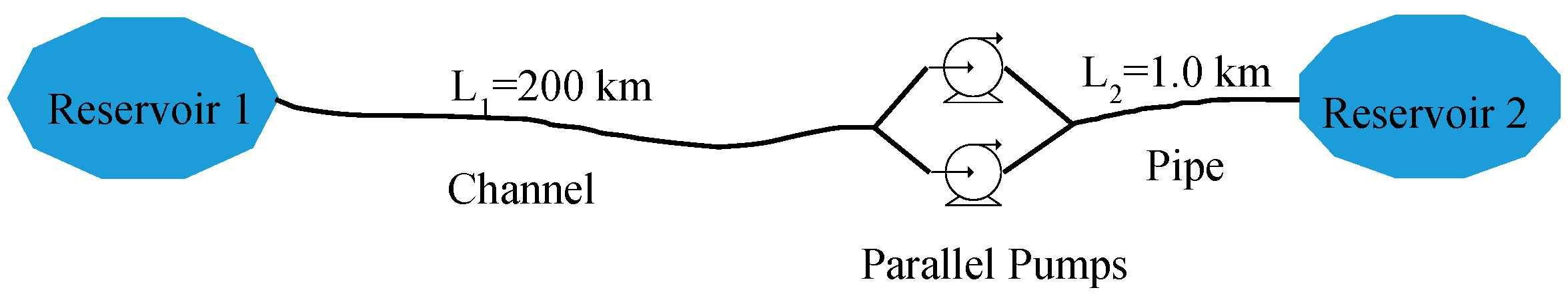
5. Application of GPU-MOC to a Long-Distance Water Transmission System

The transient of a long distance water transmission project is simulated, in which the pumping part is from an example in the book [27] by Chaudhry. We modified it by adding a long trapezoidal channel between the upstream reservoir and the pump station (Figure 7). The parameters of the project are shown in

Table 4. Computation parameters.

Pipe	Pump	Trapezoidal Channel
Length = 1000 m	QR = 0.25 m3/s	Water level of reservoir 1 = 1.5 m
D = 0.75 m	HR = 60 m	Length = 200 km, wide = 1 m
Wave speed a =1000 m/s	NR = 1100 rpm	Bottom slope = 0.0002
Q = 0.5 m3/s	WR2 = 16.85 kg∙m2	Side slopes 0.5 horizontal to 1 vertical
Friction factor = 0.012	${\eta }_R$= 0.84	Manning roughness = 0.012

. The discharge of the two parallel pumps is lumped together, and the suction lines being short are not included in the analysis. Pump trip is considered to be the cause of the transients, and there is no valve action.

The differential equations for free-surface unsteady flow are solved also by MOC [25]. An interpolation procedure is necessary so that calculations can proceed along characteristic lines. Errors are introduced in the interpolation approximation, and high order interpolation are always adopted to reduce the errors. However, the consumed time and the storage space of the simulation for high order interpolation would increase significantly. To investigate the computing efficiency of the GPU-MOC method in high order interpolation, first-order and second-order Lagrange interpolations [28] are used in simulating the transient processes of free-surface unsteady flow of this system.

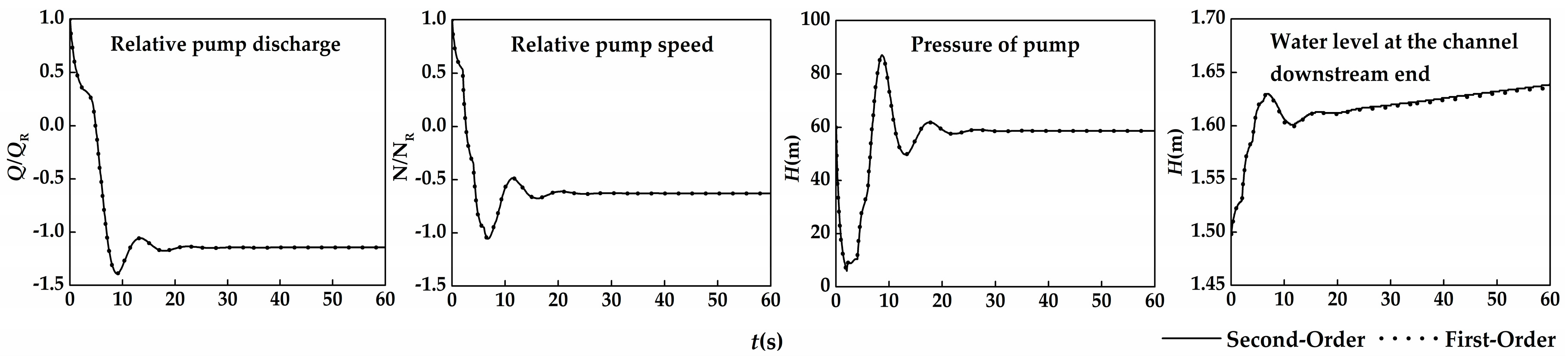
Figure 8 presents the comparisons of the history curves of pump head, discharge, speed, and head of open channel at downstream by first-order and second-order interpolations. The results of pump parameters for the two interpolations are nearly the same, because the treatments for the pressurized pipe and pump are identical, and the water level change for the open channel is small, which has little impact on pump parameters. After power is lost, the reactive torque of the liquid on the impeller causes the rotational speed to decrease, which, in turn, reduces pressure head and discharge. As a result, the discharge at the channel downstream end that delivers to the pump reduces quickly, causing the water level rises. The water levels at the channel downstream end by the two interpolation methods are different due to interpolation errors. Once the pump reaches its reverse rotating steady-state conditions, the water level at the channel downstream end increases uniformly and slowly.

The computing efficiency of the GPU-MOC in high order interpolation is analyzed. The pipe segment length is $\Delta x=1$ m, time step is $\Delta t=0.001$ s, and the corresponding section number is 201,000. The transient behavior in the system within 600 s after the pump trip is simulated. The block size is set to 256.

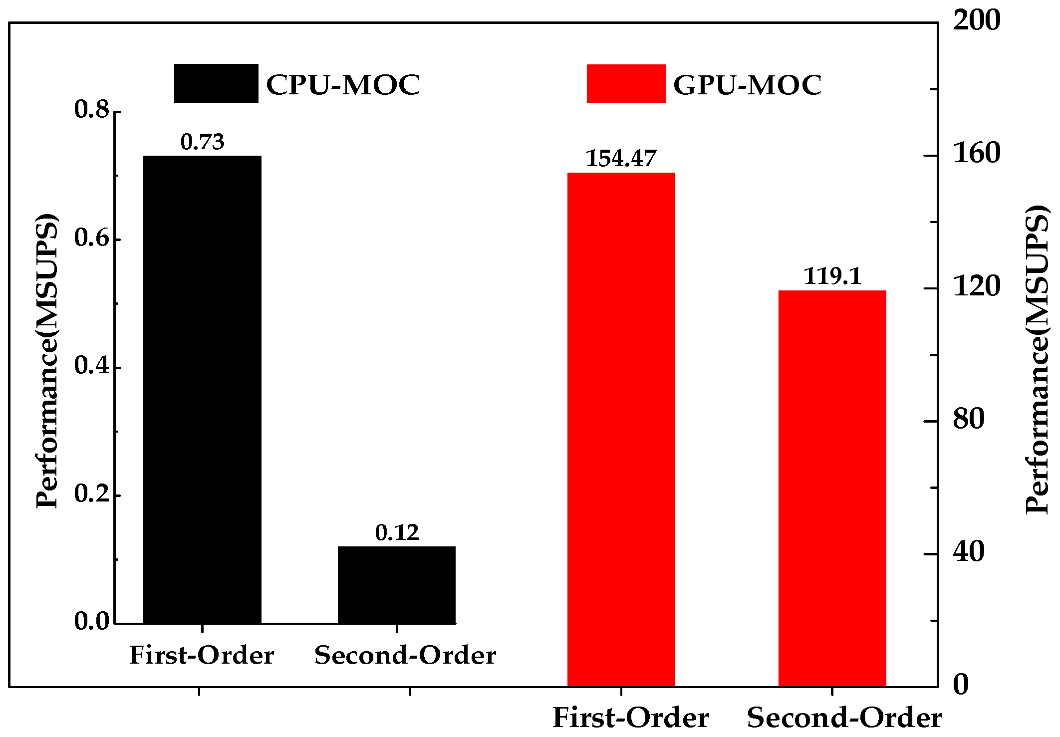
GPU-MOC method shows a great advantage in computing intensive problem, especially in high order interpolations (Figure 9). For both first-order and second-order interpolations, the performances of GPU-MOC are much better than those of CPU-MOC. Moreover, for GPU-MOC, the second-order interpolation achieves more significant performance gains compared with the first-order interpolation. For first-order interpolation, the consumed time is 45.726 hours by CPU-MOC, but only 0.217 hour by GPU-MOC, and the achieved speedup ratio is 210.7. For second-order interpolation, the consumed time is 288.9 hours by CPU-MOC, but only 0.281 hour by GPU-MOC, and the achieved speedup ratio is up to 1027. That is to say, the speedup ratio of Second-Order is 4.9 times to that of the first-order. Therefore, high-order computing methods executed on the GPU can be used in simulating large-scale practical problems for obtaining more accurate results.

6. Conclusions and Future Works

This paper presents a novel GPU implementation of MOC on single GPU card for accelerating the simulation of hydraulic transients. CPU is mainly responsible for executing logical operations and GPU is mainly responsible for executing floating operations. The MOC kernel, which is mainly responsible for calculation, is executed on GPU and invoked by an odd-even alternate form by CPU. The configuration parameters of the MOC kernel are organized as 1D linear structure to fit the line structure of the pipes.

The benchmark single pipe water hammer problem is simulated to verify the accuracy and efficiency of GPU-MOC method. It is found that the numerical results of GPU-MOC are identical with CPU-MOC, but the computational efficiency is much higher, and the obtained speedup ratios of GPU-MOC are up to hundreds compared to CPU-MOC. Two computing-intensive problems, the large-scale water distribution system and the long-distance water transmission system, are simulated, which successfully validate the high computational efficiency of the GPU-MOC method. Moreover, the GPU-MOC method can achieve more significant performance gains as the size of the problem increases. Therefore, finer calculation sections and high-order methods can be used to simulate large-scale practical problems for getting more accurate results.

The GPU-MOC method has great value for practical applications because the algorithm is simple, high-efficiency, easy to program, and convenient to popularize. Future work will focus on further optimization of the present algorithm and more computational intensive transient simulations like 2D or 3D and on multiple GPUs.