Abstract
This paper proposes a convex quadratic optimization commutation method to raise the equalization degree of power loss distribution of coil array for magnetic levitation planar motors. Starting with the modeling of electromagnetic forces/torques and commutation of coil array, the global power loss and the local power losses of coil array are analyzed, and the power loss equalizing degree is defined to evaluate the power loss distribution of coil array being commutated dynamically. Then, in consideration of the fact that the global power loss is the quadratic function of commutated coil currents, the convex quadratic function optimization with equality constraint and boundary constraints is applied to commutate the coil array, and the power loss equalizing degree is raised by decreasing the boundary constraints of optimization. Taking the magnetically levitated planar motor under investigation as examples and using quadprog routine in Matlab Optimization Toolbox, which is a dedicated quadratic optimization routine, it is verified that the power loss equalizing the degree of coil array is raised gradually and the power loss distribution of coil array becomes more uniform along with decrease of the boundary constraints. The convex quadratic optimization commutation is verified experimentally on a constructed multi-dimension force/torque measurement platform. Using the convex quadratic optimization commutation can not only improve the power loss distribution of coil array of magnetically levitated planar motors, but also make it possible to select lower capacity power amplifiers to produce the identical desired electromagnetic forces and torques.
1. Introduction
Magnetically levitated planar motors (MLPM) show promising applications in driving advanced manufacturing equipment (extreme-ultraviolet lithography, nano-imprint lithography, and other nano/micro manufacturing equipment) that are used in high-vacuum conditions, because these motors can move without any mechanical friction and wear [1,2,3]. They are mainly constituted of two typical parts: stator and mover. The stator and the mover can be collocated in two ways: the mover consists of a coil array and the stator has a permanent magnet array (MLPM with moving coils) [2,3,4,5,6], and the mover consists of a permanent magnet array and the stator consists of a coil array (MLPM with moving magnets) [1,7,8].
No matter how MLPM are configured, they can all be classified as permanent magnet synchronous motors. For these permanent magnet synchronous motors, either planar or rotary, the commutation of windings or coils is always the key link. Once these motors have been physically configured, the magnetic field distribution cannot be changed; thus, the regulation of coil or winding currents, i.e., the commutation becomes the only alternative to control these motors [7,9,10]. These coils or windings have to be commutated to provide adequate energy for six degrees of freedom (DOF) movements in three-dimension Euclidean space [11]. Moreover, these coils or windings still have to be accurately commutated so that the six-DOF movements can obtain better decoupling and controlling performances [12,13]. Figure 1 shows the basic control structure of MLPM, in which qref and q denote reference input vector and output vector, respectively; Wc and Wd denote control forces/torques and desired forces/torques, respectively, and i denotes the commutated current vector.

Figure 1.
Basic control structure including the commutation (algorithm) of coil array and the electromagnetic forces/torques model.
Different commutation methods will result in different distributions of currents and ohmic losses (refer to Joule losses or dissipated power of coils, hereinafter named power loss) among all the coils, although these currents can generate identical electromagnetic forces and torques. In the literature [10,14], a commutation method called direct wrench-current decoupling was proposed, which includes smooth switching of coil currents for MLPM with moving magnets. Using this method, wherein the coil currents are solved by the pseudo inversion of the electromagnetic force/torque coefficient matrix, the coils are commutated optimally in the sense of minimum power loss of the coil array. On the other hand, peak current is not taken into account and power loss distribution among coils usually shows disequilibrium. In page 111 of reference [14], the temperature distribution of commutated coils in some situations are measured by thermal imaging and the temperature range from 20 °C to 37.6 °C is observed among commutated coils. In reference [15], an apparent temperature distribution difference from 30 °C to 75 °C is also observed. Reference [16] illustrates a coil current distribution from 0 A to 3 A when a MLPM with moving magnets is desired to track a designed rectilinear movement. Reference [17] also illustrates the different temperature distributions from 10 °C to 60 °C. These studies indicate the obvious disequilibrium with respect to currents and power loss of coil array of MLPM.
When the power loss distribution of coil array is under a state of imbalance for a relatively long term, it may result in serious MLPM control problems. One or more coils could break down or even burn out too early because of frequent overheating and thermal shock. It could also cause irreversible demagnetization of the permanent magnets. Thus, the commutation and control precision of the motor could deteriorate or go out of control. In addition, the power loss disequilibrium of the coil array will confuse the capacity selection of the coil power amplifiers. For these reasons, in the literature [18], three norm-based commutation methods are compared and one of them—the clipped l2-norm based commutation (CL2C) method—is proposed to commutate the ironless, over-actuated electromagnetic actuators with moving magnets. The realized algorithm of CL2C method, which is based on iteration, offers the advantage of fast calculation time over quadratic programming. However, this heuristic algorithm is not inevitable to obtain the optimal solution of commutated currents.
In this paper, the distribution of currents and power loss of coil arrays take into account coils commutation, and a convex quadratic optimization commutation method is proposed to improve it. The global power loss, local power loss, and power loss equalizing degree (PLED) of coil array are defined to evaluate the power loss distribution. The approach to raising PLED is validated by giving a lower boundary constraint in the convex quadratic optimization commutation, which is implemented by using the convex optimization routine with an active-set algorithm, quadprog in Matlab Optimization Toolbox. It is also verified by measuring real electromagnetic forces and torques on the constructed force/torque measurement platform. The convex quadratic optimization commutation can obtain the optimal currents solution in the sense that power loss distribution in all the coils is balanced. In the meantime, the lower boundary constraint in the convex quadratic optimization commutation can be used to select DC (direct current) power amplifiers with lower capacities and costs.
2. Commutation and Power Loss Equalizing Degree of Coil Array
For MLPM with moving coils, its activated coils are invariant. Yet for MLPM with moving magnets, its activated coils are always varying because these coils have to be switched smoothly along with the movement of the mover. Their electromagnetic forces and torques both originate from the interactions between the current-carrying coils and the magnetic field of permanent magnets, i.e., Lorenz forces. Thus, hereafter, a being-studied MLPM with moving coils [11,12,19,20] is taken as an example to set up the commutation method. This MLPM is composed of a large area planar stator and a long x-y travel mover. It is initially designed such that the mover of 1 kg mass can obtain acceleration of 1g in x or y direction at a maximum gap of 2 mm; enough energy can be provided for the real-time control of all DOF motions. Figure 2a,b show the configurations and design parameters of the stator and mover, respectively. The designed parameters and their final dimensions after being manufactured are shown in Table 1.
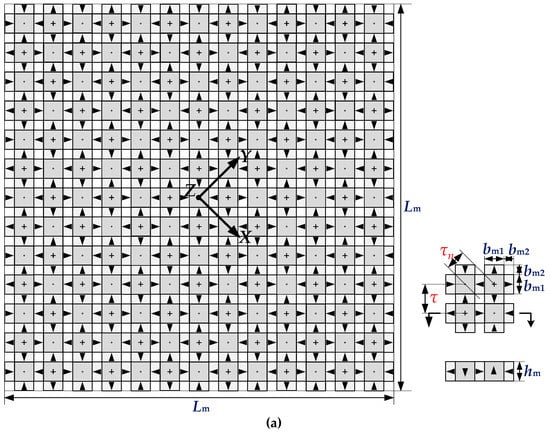

Figure 2.
Configurations and parameters of MLPM (magnetically levitated planar motor) under investigation: (a) Halbach permanent magnet array; (b) coil array.

Table 1.
Related parameters and dimensions of MLPM (magnetically levitated planar motor) under investigation.
As Figure 2a shows, the stator of MLPM is a Halbach permanent magnet array whose magnetic energy is concentrated on one side of the stator. Its magnetic flux density distribution in 3-dimension Euclidean space as a whole can be set up as a harmonic model. As Figure 2b shows, the mover of MLPM consists of four forcers arranged in a centrosymmetric order; each forcer contains five ironless coils. Twenty coils of coil array are activated respectively by 20 DC power amplifiers. The force generated from each activated coil located in the permanent magnetic field can be calculated by the Lorenz volume integral method. The two forces of each forcer generated are the summation forces of five coils generated. The three forces and three torques of the mover generated are the summation forces and torques of four forcers generated.
2.1. Commutation of Coil Array
The commutation of MLPM starts with the modeling of the electromagnetic forces and torques. As Figure 3 shows, there are two coordinate systems. One is the fixed coordinate system O-XYZ and is defined on the surface of the permanent magnet array. In this coordinate system, the three-dimension magnetic flux density distribution of the permanent magnet field can be represented analytically. The other one is the moving coordinate system o-xyz and is set up at the bottom plane of the coil array. In this coordinate system, each coil is defined. Two coordinate systems are parallel.

Figure 3.
Coordinate systems for modeling of the electromagnetic forces and torques.
Thus, the position and attitude that the mover locates in the stator can be denoted by q:
and the position and attitude that coil Cj locates in the moving coordinate system o-xyz can be denoted by qcj:
Given that the coil Cj is commutated by unit current, 1A, the x-, y-direction propulsion force Fxj (q), Fyj (q), z-direction levitation force Fzj (q), and x-, y-, z-axis torques Txj (q), Tyj (q), Tzj (q), can be integrated by using the Lorenz force volume integral method [7]. These forces and torques are denoted by:
then the electromagnetic forces and torques generated from all coils of n number, which is commutated by unit current, respectively, can be listed as a matrix of 6 × n dimensions. This matrix is denoted by K (q):
It can be seen from (4) that K(q) is a matrix of 6×n dimension and its six elements of each column represent three forces and three torques, respectively, when the coil Cj is commutated by unit current (1A). This matrixcharacterizes the force/torque coeficients of MLPM between the coil currents and the electromagnetice forces/torques, just as the torque constant of the rotating motor. However, this coeficient matrix is not a constant matrix and it is still dependent on the position and attitude vector q that the moving coordinate system o-xyz locates in the fixed coordinate system O-XYZ. Herein assuming coils of n number are commutated by current vector i:
and the mover consisting of coils of n number as a rigid body, the x-, y-, and z-direction forces Fx (q), Fy (q), and Fz (q) and x-, y-, z-axis torques Tx (q), Ty (q), and Tz (q), which act on the mover, can be added up by using the superposition principle as:
Conversely, if the desired electromagnetic forces and torques of the real-time movements in position and attitude q are:
then the commutated coil currents ic should satisfy
In light of Equation (8), the commutated coil currents ic can be derived by:
where represents an inverse computation about force/torque coeficient matrix K(q), because MLPM is usually over-actuated so as to provide adequate energy for moving in six-DOF, which implies the number of coils n is larger than the number of DOF: n > 6, K(q) is a rectangular matrix. Hence, can be solved analytically by the pseudo inverse of K(q):
and the uniquely analytical solution of commutated coil currents ic can be solved by
Equation (11) implies that the coil currents are commutated in sense of the minimum square sum of all coil currents, but that does not mean that the current squares are evenly distributed among all coils [11,19].
2.2. Power Loss Equalizing Degree and the Approach to Raise It
For the sake of derivation convenience, the commutated coil currents and the equivalent resistances of each coil are respectively denoted by icj (j = 1, 2, …, n) and Rj (j = 1, 2,…, n). Then the power loss summation of all commutated coils, which is named as the global power loss, can be calculated and denoted by Pg:
and the power loss of every coil, which is named as the local power loss, is denoted by Pj:
Then, defining an index, namely power loss equalizing degree (PLED) and denoted by Ep:
This indicates the ratio of the average to the maximum of all the local power losses.
Furthermore, letting the maximal square of commutated coil currents be denoted by Sjm
and the square sum of commutated coil currents be denoted by Sg
and then supposing the equivalent resistances of each coil are equal, PLED can be derived as:
It can be deduced from Equation (14) and Equation (17) that PLED varies between 0 to 1 and it is a dimensionless quantity; therefore, it can be identified as a normalization index to evaluate the power loss distribution of commutated coil array. The higher this normalization index is, the nearer the average and the maximum of all the local power losses are, and the more well-distributed the local power losses are.
It can also be observed from Equation (17) that there are three possible selections to raise PLED. The first one is to increase the square sum of the commutated coil currents, Sg. This is obviously inadvisable, because doing so will increase global power loss, Pg. The second selection is to decrease the coil number n. Confined to the high energy requirement and the precision motion requirement of MLPM, this selection is also inadvisable. Consequently, the only feasible selection is the third one, i.e., raising PLED by decreasing the maximal square of commutated coil currents, Sjm. In order to decrease Sjm, the maximal amplitude of commutated coil currents, max|icj| (j = 1, 2, …, n), should be reduced. Actually, this maximal amplitude is the infinite norm of commutated coil current vector:
Thus, the PLED can be raised by decreasing the infinite norm of commutated coil current vector ||ic||∞.
2.3. Raising Power Loss Equalizing Degree by Convex Quadratic Optimisation Commutation
Considering the commutated coil current vector ic
its each element, icj (j = 1, 2, …, n), is a scalar and denotes the commutated coil current value, i.e., DC or AC RMS (alternative current root mean square). This means that the set of ic is in the real domain: ic ϵ Rn. Since Rn is a convex set, ic is a convex set, too [21].
Further condidering the quadratic function f (ic):
its defining domain, i.e., the value domain of ic, is a convex set and it is twice differentiable on its defining domain. The Hessian matrix of f (ic), , can be twice differentiated as
where In is a n-dimensional unit matrix. As a result of In being a positive definite matrix, the Hessian matrix of f (ic), , is also a positive definite matrix. In light of the second order condition for function convexity [21], f (ic) is a strictly convex quadratic function.
In order to generate the desired electromagnetic forces and torques, the commutated coil currents ic must first satisfy:
In addition, for the purpose of reducing the infinite norm of commutated coil current vector, ||ic||∞, the absolute values of each element of ic an upper bound Im can be given:
where Im is a positive real number. When this upper bound Im is reduced, the infinite norm ||ic||∞ is to be decreased and PLED can be raised according to (18).
As a result of the discussions above, the problem of raising PLED by commutation can be summerized and abstracted as a convex quadratic optimisation problem:
in which the optimisation variables are the commutated coil currents, ic=(ic1, ic2, …, icn)T; the optimisation objective is to minimize the quadratic function ; and the optimisation is subject to two constraint conditions: one is the linear equlity constraint as shown in Equation (22), and another is the boundary constraint, shown in Equation (23).
3. Implementation of Raising Power Loss Equalizing Degree (PLED) by Convex Optimization Commutation
3.1. Algorithms of Convex Quadratic Optimization Commutation
As Figure 1 shows, the commutation algorithm must unite with the controllers in real-time. Since the focus of this paper is to raise PLED by convex optimization commutation instead of the real-time control, thereinafter all commutations are implemented using quadprog routine with an active-set algorithm on Matlab R2012b, Lenovo-PC with Intel(R) Core(TM) i5-3230M CPU @ 2.60 GHz.
The quadprog routine in Matlab Optimization Toolbox [22] is specifically programmed to solve the quadratic objective optimization problems with equality, inequality, and boundary constraints, in spite of these problems being convex or non-convex. This routine also facilitates users to select a few different algorithms—active-set, interior-point, and trust-region-reflective algorithms among others. These algorithms, searching for the optimal solution in the feasible region, can still converge fast and operate efficiently on a dedicated high-speed microprocessor [23,24,25,26].
3.2. Implementation of Raising PLED by Convex Quadratic Optimization Commutation
The commutated coil currents depend upon the desired electromagnetic forces and torques determined by the motion profile of MLPM. A most likely motion profile is that the coil array stage is levitated above the permanent magnet array stage and moves straight from one point to another in the horizontal direction. Supposing the coil array stage is levitated above the permanent magnet array stage at the air gap of 1 mm (the working air gap of the MLPM under investigation), and moves at the acceleration of 1g in x-direction ranging from −10.61 mm to 10.61 mm (y = 10.61 mm), the desired electromagnetic force/torque vector Wd can be calculated as:
While the coil currents are calculated according to Equation (9), i.e., the coils are commutated according to the optimization commutation as shown in Equation (24), without any boundary constraints, the commutated currents of four forcers are as shown in Figure 4. From this figure, it can be observed that the commutated currents are seriously imbalanced. The current amplitudes of forcer I and forcer III are relatively higher, the current amplitudes of forcer II and forcer IV are relatively lower, and the maximum and minimum amplitudes of commutated currents are 3.0 A and 0.18 A, respectively. Due to these unbalanced current amplitudes, the power loss distribution among the four forcers as well as among all coils will be seriously imbalanced.
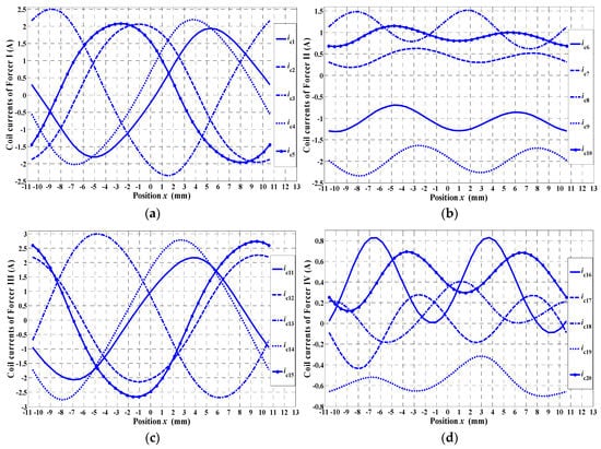
Figure 4.
Coil currents of (a) Forcer I, (b) Forcer II, (c) Forcer III, and (d) Forcer IV by optimization commutation without boundary constraint Im.
While the coils are commutated by the optimization commutation with boundary constraint Im = 2.0 A, the commutated currents of four forcers are as shown in Figure 5. It can be observed from this figure that the maximum current amplitudes of four forcers are limited within 2.0 A and all commutated currents of the four forcers are inclined towards a more equalizing trend.

Figure 5.
Coil currents of (a) Forcer I, (b) Forcer II, (c) Forcer III, and (d) Forcer IV by optimization commutation with boundary constraint Im = 2.0 A.
When the maximum current amplitude is limited by the optimization commutation, the maximum local power loss is reduced and thus, the PLED is raised. Figure 6 shows the PLED curves when commutations are optimized without boundary constraint Im and with boundary constraint Im = 2.6 A, 2.4 A, 2.2 A, 2.0 A, respectively. It can be seen from Figure 6 that PLED is raised in whole x-direction ranging from -10.61mm to 10.61mm, along with decrease of boundary constraint Im.
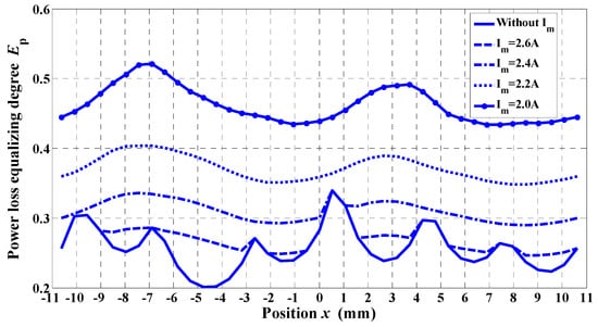
Figure 6.
Power loss equalizing degree when the commutations are optimized without boundary constraint Im, with boundary constraint Im = 2.6 A, 2.4 A, 2.2 A, and 2.0 A, respectively.
When the commutations are optimized without boundary constraint Im and with boundary constraint Im = 2.6 A, 2.4 A, 2.2 A, 2.0 A, respectively, the local power loss distributions in position x = −6.896 mm and x = −4.774 mm, which are the maximum and minimum PLED positions, are as shown in Figure 7, respectively. It can be seen from Figure 7 that the maximum local power loss is gradually reduced and the local power loss distribution becomes more and more uniform, along with decrease of boundary constraint Im.
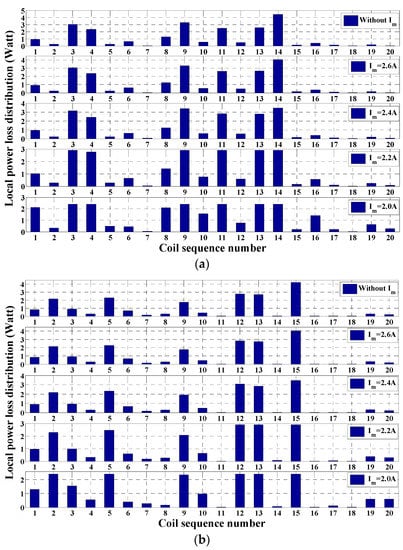
Figure 7.
Local power loss distribution in position (a) x = −6.896 mm and (b) x = −4.774 mm when commutations are optimized without boundary constraint Im, with boundary constraint Im = 2.6 A, 2.4 A, 2.2 A, and 2.0 A, respectively.
When MPLM runs in real time, all the six-DOF movements of the mover have to be controlled completely. Therefore, efforts taken to control the six-DOF movements should be taken into account. Supposing the mover is levitated above the stator at air gap of 1 mm, and moves at acceleration of 1g in the x-direction, ranging from -10.61 mm to 10.61 mm, the desired electromagnetic force/torque vector including control efforts, Wd, is:
When the commutations are optimized without boundary constraint Im, with boundary constraint Im = 2.9 A, 2.6 A, 2.3 A, and 2.0 A, respectively, the PLED curves are as shown in Figure 8. As observed from this figure, along with the decrease of the boundary constraint Im, the PLED is gradually raised in the x-direction, ranging from −10.61 mm to 10.61 mm (y = 10.61 mm).
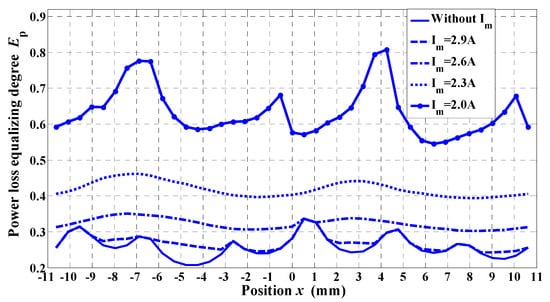
Figure 8.
Power loss equalizing degree when the commutations are optimized without boundary constraint Im, with boundary constraint Im = 2.9 A, 2.6 A, 2.3 A, and 2.0 A, respectively.
Likewise, when the commutations are optimized without boundary constraint Im, with boundary constraint Im = 2.9 A, 2.6 A, 2.3 A, and 2.0 A, respectively, the local power loss distributions in position x = −4.244 mm and x = 4.244 mm, which are the maximum and minimum PLED positions, are as shown in Figure 9, respectively. It can be seen from Figure 9, along with the decrease of the boundary constraint Im, the maximum local power loss is gradually reduced and the local power loss distribution becomes more uniform.

Figure 9.
Local power loss distribution in position (a) x = −4.244 mm and (b) x= 4.244 mm when commutations are optimized without boundary constraint Im, with boundary constraint Im = 2.9 A, 2.6 A, 2.3 A, and 2.0 A, respectively.
From the results of Figure 6 and Figure 8, it can be concluded that PLED of coil array can be gradually raised by decreasing the boundary constraint of convex quadratic objective optimization. While PLED is being raised, the local power loss distribution of coil array becomes more uniform, as is shown in Figure 7 and Figure 9.
Figure 10 shows the varying trends of PLED while the boundary constraint Im is being decreased gradually from 3.2 A to 2.0 A, in which the x-direction positions are corresponding to Figure 7 and Figure 9, i.e., x = −6.896 mm, −4.774 mm, −4.244 mm, 4.244 mm, respectively. From Figure 10, it can still be observed that the lower the boundary constraint Im, the faster PLED grows, and that the higher the boundary constraint Im, the slowly PLED grows.
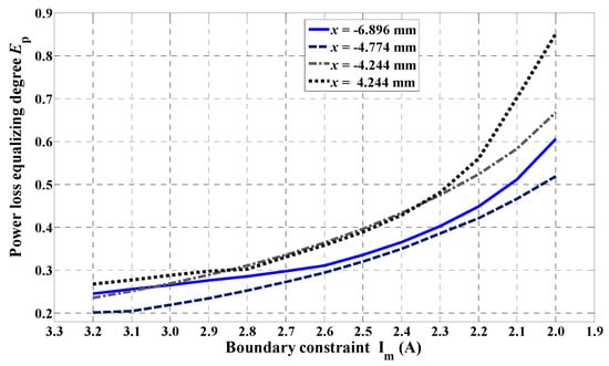
Figure 10.
PLED varying trends while the boundary constraint Im is being gradually decreased from 3.2 A to 2.0 A.
4. Experimental Verification of Convex Quadratic Optimization Commutation
4.1. Configuration of Comprehensive Measurement Platform (System)
In order to verify the electromagnetic force/torque model and the commutation algorithm of MLPM, a comprehensive measurement platform (system) was set up. Figure 11 and Figure 12 show the photograph and the configuration of the measurement platform, respectively. The key device of the measurement platform is a multi-dimension force/torque sensor, which has its own graphical user interface (SMART300, manufactured by Hefei Sunsor Technology Co. Ltd., Hefei, China). This sensor works on the basis of the stress-strain theory and its measurement is seldom affected by magnetic hysteresis. This sensor can simultaneously measure three force components and three torque components in a three-dimension Euclidean space. Measured data of electromagnetic forces and torques are pre-processed by the multi-dimension force/torque sensor itself and then transmitted to the host computer, where it can be displayed and analysed.
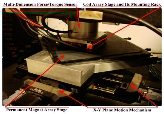
Figure 11.
Photograph of comprehensive measurement platform (system).
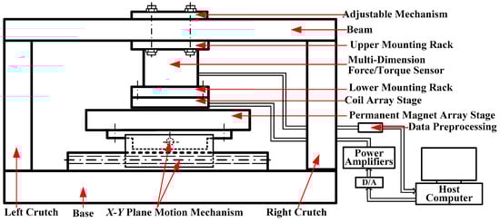
Figure 12.
Configuration of comprehensive measurement platform (system).
Permanent magnets are fixed on one base to constitute the permanent magnet array stage. The surface of the permanent magnet array is coated with epoxy resin adhesive to keep the planeness of the array. Twenty coils are fixed on one base to constitute the coil array stage and its surface is also coated with epoxy resin adhesive to guarantee the planeness. These two coatings take into account the gap between the coil array and the permanent magnet array. Twenty coils of the coil array stage are actuated respectively by 20 DC power amplifiers. The output currents of all amplifiers are controlled by the host computer via a D/A converter.
As is shown in Figure 11 and Figure 12, the multi-dimension force/torque sensor is mounted on a beam via an upper mounting rack. The coil array stage is connected with the sensor via the lower mounting rack. An adjustable mechanism adjusts the sensor’s height so that the gap between the two arrays can be changed. The permanent magnet array stage is mounted on an X-Y plane motion mechanism, which is driven by two controlled step motors and thus the relative position of two stages in the horizontal direction can be controlled by its graphical user interface on the host computer. To eliminate disturbance of the coil cable, the permanent magnet array stage instead of the coil array stage moves relatively; the coil array stage and the sensor are always stationary. This does not change the relative motion relationship between the two stages.
After the measurement platform is accurately calibrated, the position precision can attain a μm order. The current precision of power amplifier can attain an mA order. The real force and torque resolutions of the multi-dimension force/torque sensor are ± 0.5 N and ± 50 N·mm, respectively.
4.2. Verification Schem and Measurement Results
As the motion of MLPM under investigation has not been controlled in real time, the static measurement scheme is adopted to verify the proposed convex quadratic optimization commutation method. This scheme has five steps: 1) Using the adjustable mechanism, ensure the gap between two stages to be z = 1 mm; 2) using the X-Y plane motion mechanism, adjust and ensure the relative position of two stages in the horizontal direction; 3) using the Matlab routine quadprog on the host computer, calculate the coil currents that can generate the desired electromagnetic forces/torques in present position; 4) using the D/A converter and power amplifiers, give the just-calculated currents to the coils and ensure the coils are actuated; 5) using the multi-dimension force/torque sensor, the generated electromagnetic forces and torques are measured in present position and under present coil currents. Sampling frequency of measurement data of the sensor is at 250 Hz and the measurement time of each point is 2 seconds at least.
Figure 13 shows the measured results of one point electromagnetic forces and torques. It can be observed that the force precision is about ± 0.5 N and torque precision is less than ±60 N·mm. Table 2 shows the coil currents solved by the convex quadratic optimization commutation method when the desired electromagnetic forces and torques are Wd = (Fxd, Fyd, Fzd, Txd, Tyd, Tzd)T = (10N, 0, 10N, 0, 0, 0)T, supposing the air gap z = 1 mm and the coil array stage, respectively, locates in 17 positions in the x-direction, ranging from −10.61 mm to 10.61 mm (y = 10.61 mm). These coil currents are solved on the host computer by the Matlab routine quadprog, where the current boundary constraints are given as Im = 2.0 A.
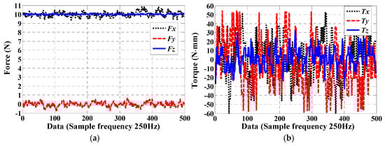
Figure 13.
One point measured data: (a) Electromagnetic forces Fx, Fy, and Fz; (b) electromagnetic torques Tx, Ty, and Tz.
Table 2.
Coil currents solved by the convex quadratic optimization commutation method when the desired electromagnetic forces and torques are Wd = (Fxd, Fyd, Fzd, Txd, Tyd, Tzd)T = (10N, 0, 10N, 0, 0, 0)T, supposing the air gap z = 1 mm and the coil array stage, respectively, located in 17 positions in the x-direction, ranging from −10.61 mm to 10.61 mm (y = 10.61 mm).
Figure 14 shows the measured results of electromagnetic forces and torques of 17 different points in the x-direction, ranging from −10.61 mm to 10.61 mm (y = 10.61 mm) when the coils are actuated according to the currents as shown in Table 2. It can be observed from Figure 14 that the desired electromagnetic forces and torques are generated when the coils are actuated by the currents calculated by the proposed convex quadratic optimization commutation algorithm. The force ripples are within ± 0.5 N and the torque ripples are about ± 50 N·mm. These ripples result from measurement errors of the multi-dimension force/torque sensor, the current errors, and the position errors between the coil array and the permanent magnet array.
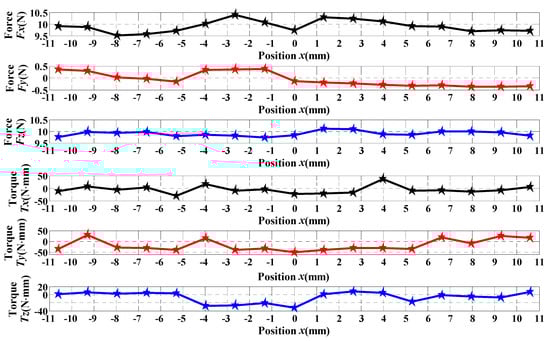
Figure 14.
Results of 17 measured points of electromagnetic forces and torques when the desired electromagnetic forces/torques are Wd = (Fxd, Fyd, Fzd, Txd, Tyd, Tzd)T = (10 N, 0, 10 N, 0, 0, 0)T.
More measurements like the ones above are taken in other positions, wherein the coil array stage is located in different y-direction positions relative to the permanent magnet array stage at the X-Y plane. These measured results indicate that the proposed convex quadratic optimization commutation method is feasible and effective. In addition, these measurement results also imply that coil power amplifiers with lower capacities can be selected to actuate the coils and generate the identical desired electromagnetic forces and torques.
5. Further Discussion about Raising PLED by Convex Quadratic Optimization Commutation
Although the decrease of boundary constraint Im of optimization commutation can raise PLED, this decrease is not boundless and PLED cannot be raised unlimitedly. Figure 15 shows the commutated currents of four forcers by optimization commutation with the boundary constraint Im = 1.95 A, which are expected to generate electromagnetic forces and torques Wd = (11 N, 1 N, 11 N, 10 N·mm, 10 N·mm, 10 N·mm)T. As observed from this figure, the commutated currents of many coils in position x = −6.896 mm and x = 3.713 mm are zero, so they cannot produce any desired electromagnetic force or torque. Figure 16 shows the electromagnetic forces and torques generated from the optimization commutation currents with boundary constraint Im = 1.95 A.
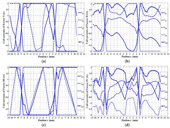
Figure 15.
Coil currents of (a) Forcer I, (b) Forcer II, (c) Forcer III, and (d) Forcer IV by optimization commutation with boundary constraint Im = 1.95 A.
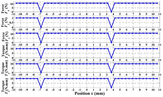
Figure 16.
Electromagnetic forces and torques generated from optimization commutation currents with boundary constraint Im = 1.95 A.
It can be seen from Figure 15 and Figure 16 that the optimization cannot obtain a feasible solution when the boundary constraint Im is less than 1.95 A. This indicates that the boundary constraint Im should have the lowest bound, which can guarantee the generation of desired electromagnetic forces and torques. This lowest bound, of course, depends upon the desired electromagnetic forces and torques. As far as two examples in this paper are concerned, the lowest bound of boundary constraint is 1.95 A. It is about 65% of 3.0 A, which is the maximum amplitude current when the commutation is optimized without the boundary constraint.
On one hand, the existence of the lowest bound limits further increase of the PLED. On the other hand, when the lowest bound of boundary constraint is determined, the capacity of coil power amplifiers can be consequently selected. In the two examples given in Section 3.2, the coil power amplifier capacity can be selected as 2.0 A. If not, it has to be 3 A at least, and this will greatly increase costs, because 20 coil power amplifiers of the same capacity are required.
6. Conclusions
This paper focuses on studying the power loss distribution of coil array and raising the uniformity of the power loss distribution among all the coils by convex quadratic optimization commutation for magnetic levitation planar motors. The commutated coil currents not only determine the electromagnetic forces and torques but also the local power loss distribution of coil array. For the sake of quantificational evaluation of the power loss distribution of coil array, the power loss equalizing degree (PLED) index is abstracted and defined at first. In order to raise the PLED, the coil array is commutated by an optimization method, which is an object optimization problem with equality constraint and boundary constraint for convex quadratic functions. When the optimization commutation is given a lower boundary constraint, the power losses of some coils are limited within a lower value; when the power losses of some other coils are increased, the PLED of all the coils is raised. This optimization commutation is implemented on Matlab by convex quadratic optimization with active-set algorithm, quadprog, and is validated on the multi-dimension force/torque sensor-centric measurement platform. Simulation examples indicate that PLED is raised gradually and the power loss distribution of coil array becomes more uniform, along with decrease in the boundary constraint of convex quadratic optimization. However, further discussions indicate that the power loss equalizing degree cannot be raised unboundedly and there exists a lowest bound of boundary constraint. This lowest bound is still dependent upon the desired electromagnetic forces and torques and can be used to select the capacity of coil power amplifiers. Further study will focus on configuring the real-time motion control platform and verifying the optimization commutation method in a real-time motion control system.
Author Contributions
Conceptualization, S.Z.; Validation, J.H. and J.Y.; Formal Analysis, S.Z.; Resources, J.H.; Writing-Original Draft Preparation, S.Z.; Writing-Review & Editing, S.Z., J.H. and J.Y.; Supervision, S.Z.; Project Administration, S.Z.; Funding Acquisition, S.Z., J.H. and J.Y.
Funding
This work was supported by the National Natural Science Foundation of China (Grant No. 51465053).
Conflicts of Interest
The authors declare no conflict of interest.
References
- Kim, W.J. Nanoscale Dynamics, Stochastic Modelling, and Multi-Scale Control of a Planar Magnetic Levitator. Int. J. Control Autom. 2003, 3, 1–10. [Google Scholar]
- Compeer, J.C. Electro-Dynamic Planar Motor. Precis. Eng. 2004, 28, 171–180. [Google Scholar] [CrossRef]
- Zhang, H.; Kou, B.; Zhang, H.; Jin, Y. A Three-Degree-of-Freedom Short-Stroke Lorentz-Force-Driven Planar Motor Using a Halbach Permanent-Magnet Array with Unequal Thickness. IEEE Trans. Ind. Electron. 2015, 62, 3640–3650. [Google Scholar] [CrossRef]
- Guo, L.; Zhang, H.; Galea, M.; Li, J.; Gerada, C. Multiobjective Optimization of a Magnetically Levitated Planar Motor with Multilayer Windings. IEEE Trans. Ind. Electron. 2016, 63, 3522–3532. [Google Scholar] [CrossRef]
- Zhang, H.; Kou, B. Design and Optimization of a Lorentz-Force-Driven Planar Motor. Appl. Sci. 2017, 7, 7. [Google Scholar] [CrossRef]
- Zhu, Y.; Yuan, D.; Zhang, M.; Liu, F.; Hu, C. A Unified Wrench Model of an Ironless Permanent Magnet Planar Motor with 2D Periodic Magnetic Field. IET Electr. Power Appl. 2017, 12, 423–430. [Google Scholar] [CrossRef]
- Jansen, J.W.; Lierop, C.M.M.; Lomonova, E.A.; Vandenput, A.J.A. Modeling of Magnetically Levitated Planar Actuators with Moving Magnets. IEEE Trans. Magn. 2007, 43, 15–25. [Google Scholar] [CrossRef]
- Boeij, J.; Lomonova, E.A.; Duarte, J.L. Contactless Planar Actuator with Manipulator: A Motion System without Cables and Physical Contact between the Mover and the Fixed World. IEEE Trans. Ind. Appl. 2009, 45, 1930–1938. [Google Scholar] [CrossRef]
- Kou, B.; Xing, F.; Zhang, L.; Zhang, C.; Zhou, Y. A Real-Time Computation Model of the Electromagnetic Force and Torque for a Maglev Planar Motor with the Concentric Winding. Appl. Sci. 2017, 7, 98. [Google Scholar] [CrossRef]
- Lierop, C.M.M.; Jansen, J.W.; Damen, A.A.H.; Lomonova, E.A.; Bosch, P.P.J.; Vandenput, A.J.A. Model-Based Commutation of a Long-Stroke Magnetically Levitated Linear Actuator. IEEE Trans. Ind. Appl. 2009, 45, 1982–1990. [Google Scholar] [CrossRef]
- Zhu, Y.; Zhang, S.; Mu, H.; Yang, K.; Yin, W. Augmentation of Propulsion Based on Coil Array Commutation for Magnetically Levitated Sage. IEEE Trans. Magn. 2012, 48, 31–37. [Google Scholar] [CrossRef]
- Zhang, S.; Zhu, Y.; Mu, H.; Yang, K.; Yin, W. Decoupling and Levitation Control of a Six-Degree-of-Freedom Magnetically Levitated Stage with Moving Coils Based on Commutation of Coil Array. Proc. Inst. Mech. Eng. 2012, 226, 875–886. [Google Scholar] [CrossRef]
- Xing, F.; Kou, B.; Zhang, L.; Yin, X.; Zhou, Y. Design of a Control System for a Maglev Planar Motor Based on Two-Dimension Linear Interpolation. Energies 2017, 10, 1132. [Google Scholar] [CrossRef]
- Jansen, J.W. Magnetically Levitated Planar Actuator with Moving Magnets: Electromechanical Analysis and Design. Ph.D. Thesis, Eindhoven University of Technology, Eindhoven, The Netherlands, 2007. [Google Scholar]
- Rovers, J.M.M.; Stöck, M.; Jansen, J.W.; Lierop, C.M.M.; Lomonova, E.A.; Perriard, Y. Real-Time 3D Thermal Modeling of a Magnetically Levitated Planar Actuator. Mechatronics 2013, 23, 240–246. [Google Scholar] [CrossRef]
- Rovers, J.M.M.; Jansen, J.W.; Compter, J.C.; Lomonova, E.A. Analysis Method of the Dynamic Force and Torque Distribution in the Magnet Array of a Commutated Magnetically Levitated Planar Actuator. IEEE Trans. Ind. Electron. 2012, 59, 2157–2166. [Google Scholar] [CrossRef]
- Rovers, J.M.M.; Jansen, J.W.; Lomonova, E.A. Multiphysical Analysis of Moving-Magnet Planar Motor Topologies. IEEE Trans. Magn. 2013, 49, 5730–5741. [Google Scholar] [CrossRef]
- Gajdusek, M.; Damen, A.A.H.; Bosch, P.P.J. l∞-Norm and Clipped l2-Norm Based Commutation for Ironless over-Actuated Electromagnetic Actuators. In Proceedings of the XIX International Conference on Electrical Machines, Rome, Italy, 6–8 September 2010; pp. 1–6. [Google Scholar]
- Zhang, S.; Zhu, Y.; Yin, W.; Yang, K.; Zhang, M. Coil Array Real-Time Commutation Law for a Magnetically Levitated Stage with Moving Coils. J. Mech. Eng. 2011, 47, 180–185. [Google Scholar] [CrossRef]
- Zhang, S.; Dang, X.; Wang, K.; Huang, J.; Yang, J.; Zhang, G. An Analytical Approach to Determine Coil Thickness for Magnetically Levitated Planar Motors. IEEE-ASME Trans. Mechatron. 2017, 22, 572–580. [Google Scholar] [CrossRef]
- Stephen, B.; Lieven, V. Convex Optimization, 1st ed.; Cambridge University Press: Cambridge, UK, 2004; pp. 21–23, 69–71. ISBN 978-0-521-83378-3. [Google Scholar]
- The MathWorks, Inc. Optimization ToolboxTM User’s Guide 2012b; The MathWorks, Inc.: Natick, MA, USA, 2012. [Google Scholar]
- Yuan, G.; Wei, Z.; Zhang, M. An Active-Set Projected Trust Region Algorithm for Box Constrained Optimization Problems. J. Syst. Sci. Complex. 2015, 28, 1128–1147. [Google Scholar] [CrossRef]
- Frank, E.C.; Zheng, H.; Daniel, P.R. A Globally Convergent Primal-Dual Active-Set Framework for Large-Scale Convex Quadratic Optimization. Comput. Optim. Appl. 2015, 60, 311–341. [Google Scholar]
- Bemporad, A. A Quadratic Programming Algorithm Based on Nonnegative Least Squares with Applications to Embedded Model Predictive Control. IEEE Trans. Autom. Control 2016, 61, 1111–1116. [Google Scholar] [CrossRef]
- Wang, X.; Yuan, Y.X. A Trust Region Method Based on a New Affine Scaling Technique for Simple Bound Optimization. Optim. Method Softw. 2013, 28, 871–888. [Google Scholar] [CrossRef]
© 2018 by the authors. Licensee MDPI, Basel, Switzerland. This article is an open access article distributed under the terms and conditions of the Creative Commons Attribution (CC BY) license (http://creativecommons.org/licenses/by/4.0/).