The Influence of Laser Linewidth on the Brillouin Shift Frequency Accuracy of BOTDR

Featured Application

Brillouin-based distributed optical fiber sensing technology, such as BOTDR, BOTDA, BOCDR, BOCDA.

Abstract

This paper analyzes the influence of laser linewidth on the measurement accuracy of a frequency-scanning Brillouin optical time domain reflectometer (FS-BOTDR), allowing for both the width of Brillouin gain spectrum and the signal-to-noise ratio (SNR) of the BOTDR system. The measurement accuracy of the Brillouin frequency shift (BFS) is theoretically investigated versus the duration of the probe pulse and the linewidth of the laser source, by numerically simulating how a FS-BOTDR works and evaluating the Brillouin gain spectrum (BGS) width and the system SNR. The simulation results show that the BFS accuracy is improved as the laser linewidth becomes narrower when the probe pulse width is fixed. We utilize five types of lasers with respective linewidths of 1.05 MHz, 101 kHz, 10.2 kHz, 3.1 kHz, and 98 Hz to compare the BFS measurement accuracy over a ~10 km optical sensing fiber. The experimental results demonstrate that the root-mean-square error (RMSE) of BFS decreases with the laser linewidth narrowing from 1.05 MHz to 3.1 kHz, which is in good agreement with the numerical simulation. However, the RMSE of BFS increases when the laser linewidth is less than 3.1 kHz, which may arise from the coherent Rayleigh noise due to a too narrow laser linewidth. The results can provide a theoretical basis and experimental guidance for choosing the appropriate laser linewidth in BOTDR.

1. Introduction

Brillouin optical time domain reflectometer (BOTDR) was firstly proposed as continuously-distributed optical fiber sensing technology in 1993 [1]. In recent decades, it has attracted much attention due to its advantages of long-distance measurement, corrosion resistance, anti-electromagnetic interference, and one-end access especially [2,3,4]. Meanwhile, with the development of its capacity of simultaneous measurement of strain and temperature [5,6], BOTDR has been more and more widely utilized in many industrial applications, such as monitoring operation status and structural health conditions of transmission lines, soil slopes, large-scale bridges, gas/oil pipelines, transportation tunnels, and underground mines [7,8,9,10]. Consequently, the measurement accuracy of Brillouin frequency shift (BFS), which determines the temperature and strain accuracy, has inevitably been a focused issue for performance enhancement of BOTDR.

The measurement accuracy of BFS can be affected by numerous factors, such as the fitting algorithm for Brillouin gain spectrum (BGS), the features of probe pulses, and even the characteristics of the laser source. Hence, a large number of papers have focused on above factors to discuss and improve the accuracy of BOTDR. Originally, a simple Levenberg-Marquart algorithm was used for BGS fitting [11]. Then, a series of time-frequency analysis methods called Cohen’s class were proposed for the signal processing of BOTDR, reducing the BFS fluctuation by three times [12]. For improving both the measurement accuracy and data processing speed, a similarity matching method was proposed, making the standard derivation of BFS results three times better [13]. An iterative quadratic fitting method can also be utilized to extract BFS from noisy signals for improvement of the BFS accuracy [14]. Besides, the features of probe light pulses also have a significant influence on the accuracy of BFS, including the pulse shape and pulse extinction ratio. Hao et al. analyzed the effects of different modulated pulse on the backscattered Brillouin power spectra of BOTDR, including the pulse shapes of Lorentzian, Gaussian, hyperbolic-secant, super Gaussian, triangular, and rectangular pulses [15,16]. The pulse sequences were complementarily coded in a BOTDR scheme to achieve a high measurement accuracy and fast measurement speed [17]. The simplex pulse codes were also testified to be beneficial for improving the signal-to-noise ratio ratio (SNR) of the BOTDR signal and the measurement accuracy of BFS [18]. The higher extinction ratio of the probe pulses was capable of enhancing the SNR as well as reducing the measurement uncertainty of BFS [19,20]. Moreover, it is noted that the wavelength and linewidth of the laser source likewise impact BFS accuracy. Lalam et al. used a wavelength diversity technique with a Brillouin ring laser in a conventional BOTDR system to improve SNR [21]. A multi-wavelength heterodyne-detection technique was utilized to provide 4.2 dB SNR enhancement, enabling the measurement accuracy to be increased by two times [22]. As an important parameter of the laser, the wide linewidth imposes a broadening effect on BGS, which affects the BFS accuracy partly, but the broadening effect is indistinctive when the laser linewidth is less than 1 MHz [23]. Meanwhile, it has been proven that the BFS accuracy is determined not only by the width of BGS, but also by the SNR of the BOTDR system [24]. The system SNR of BOTDR is inherently related with the laser linewidth closely, because the coherent heterodyne detection, which is sensitive to the laser linewidth, is commonly used in BOTDR [25]. Hence, the influence of the laser linewidth on the BFS accuracy of BOTDR needs to be further discussed in detail, considering both the BGS width and the system SNR.

In this paper, how the BFS accuracy is determined by the linewidth of the laser source is theoretically analyzed and experimentally verified in a frequency-scanning BOTDR (FS-BOTDR). The broadening effect of BGS was analyzed, allowing for both the pulse width of the probe light and the frequency-scanning process in an FS-BOTDR. Then, the SNR of BOTDR with coherent heterodyne detection was calculated, treating the phase fluctuation as the primary noise source. The BFS accuracy was finally simulated numerically taking into account both the BGS and the SNR synthetically. We used five lasers with respective linewidths of 1.05 MHz, 101 kHz, 10.2 kHz, 3.1 kHz, and 98 Hz to perform temperature measurement in the BOTDR sensing system and verify the numerical simulation. The results of this research will be helpful to choose the laser linewidth for the BOTDR.

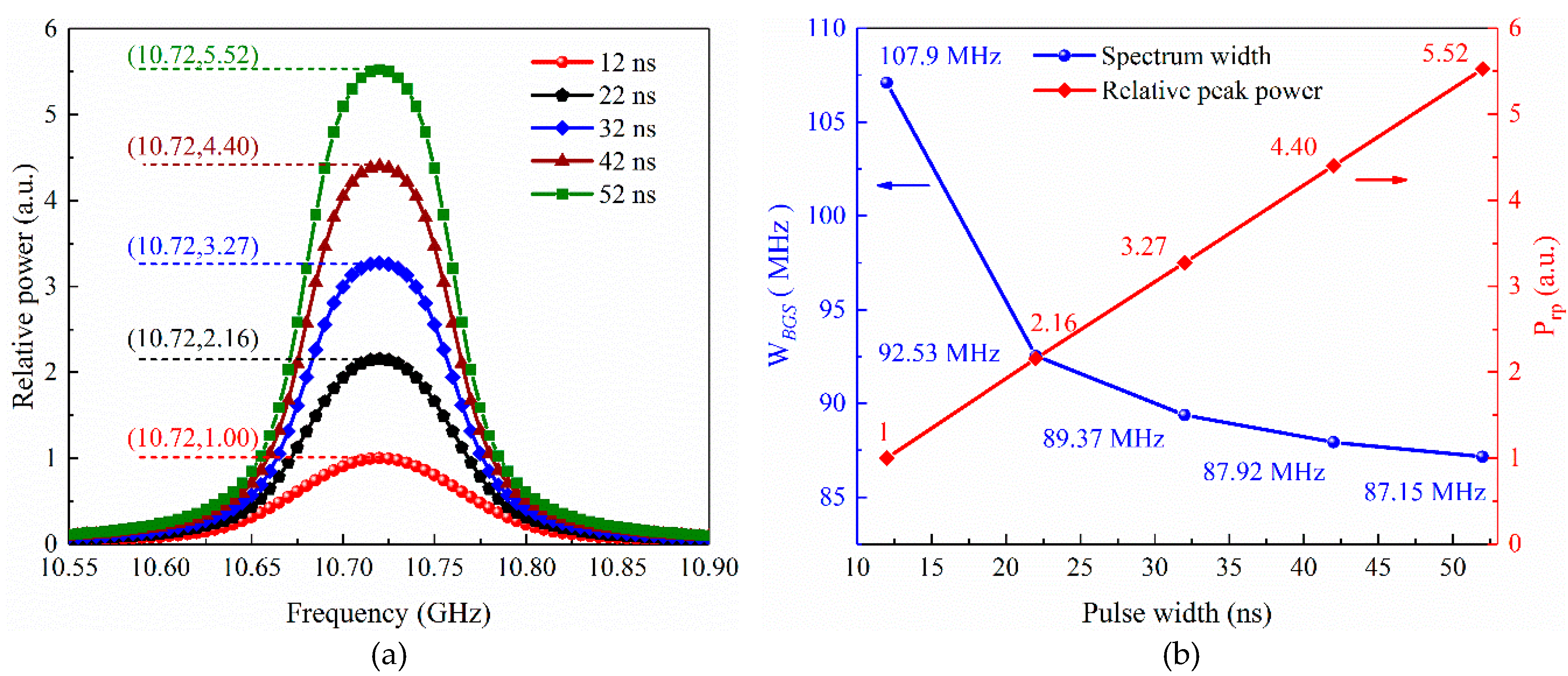
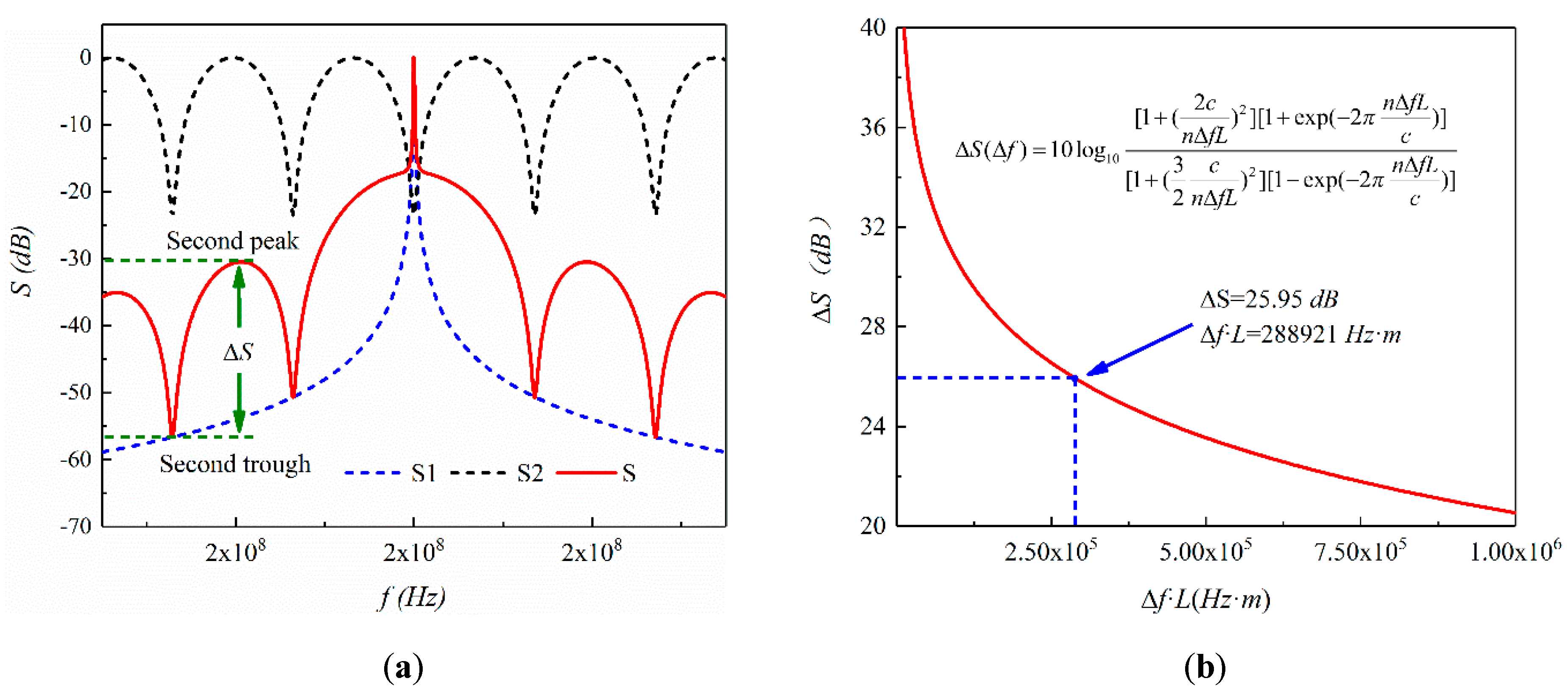
2. Numerical Simulation

Figure 1 gives a classical schematic diagram of BOTDR with coherent heterodyne detection [26]. One branch of the seed laser is modulated by an optical modulator to generate probe pulse light, which is injected into the tested fiber through an optical circulator. The other one branch passing a polarization controller is injected into a photodetector to beat with the Brillouin backscattering. The output electronic signal is orderly down-converted by mixing with a frequency scanner, filtered by a band-pass filter (BPF), and acquired by a data acquisition (DAQ) digitalizer.

The measurement error of BFS in FS-BOTDR is related with both the width of BGS denoted as W_BGS and the system SNR, which is given by Equation (1) [1]:

$$\Delta \alpha =\frac{W_{\mathrm{BGS}}}{\sqrt{2}{(SNR)}^{1/4}}$$

(1)

hence, the values of W_BGS and SNR need to be both analyzed for figuring out the BFS accuracy of Δα, as specified below.

When the continuous lightwave is injected into the tested fiber, the obtained BGS presents a Lorentzian shape, given by [27]:

$$G_{\mathrm{B}}(f)=g_0\frac{{(w/2)}^2}{{(f-f_{\mathrm{B}})}^2+{(w/2)}^2}$$

(2)

where w is the full-width at half maximum (FWHM) of BGS, f_B is the Brillouin frequency shift, and g₀ is the Brillouin gain coefficient, which is the BGS peak value when f = f_B.

When the continuous lightwave is modulated into the pulse light with a peak power of P₀ and pulse width of τ, the power spectrum of the pulse probe light can be expressed as:

$$P_{\mathrm{p}}(f,f_{.0})=P_0{[\frac{\sin \pi (f-f_0)\tau }{\pi (f-f_0)}]}^2,$$

(3)

where f₀ is the optical frequency of the probe light. Hence, the Brillouin backscattered-light power spectrum for pulse light can be calculated by [24]:

$$Q_{\mathrm{B}}(f)={\displaystyle {\int }_{-\infty }^{+\infty }{P}_{\mathrm{p}}(f,f_0)}{G}_{\mathrm{B}}(f)=\frac{g_0{P}_0\tau }{{\eta }^2+1}\left\{1+\frac{{\eta }^2-1-e^{-\tau w\pi }[({\eta }^2-1)\cos \tau w\eta \pi +2\sigma \sin \eta \tau w\pi ]}{\tau w({\eta }^2+1)\pi }\right\}$$

(4)

where:

$$\eta =\frac{f-f_B}{w/2}$$

(5)

In the FS-BOTDR, the power spectrum, Q_B(f), is always measured by the frequency-scanning method. When the frequency scanner is tuned at a certain frequency point, the integrated power of every frequency segment passing the BPF is acquired by DAQ. Hence, as the frequency scanner is tuned step by step, the final measured spectrum after frequency-scanning process, denoted as H_B(f, N), can be given by:

$$H_{\mathrm{B}}(f,N)=\{Q_{\mathrm{B}}^1(f),Q_{\mathrm{B}}^2(f),\dots ,Q_{\mathrm{B}}^{\mathrm{N}}(f)\}$$

(6)

$$Q_{\mathrm{B}}^i(f)={\displaystyle {\int }_{f_s+(i-1)f_{\mathrm{step}}-B/2}^{f_s+(i-1)f_{\mathrm{step}}+B/2}{Q}_{\mathrm{B}}^{}(f)}df,i=1,2,\dots ,N.$$

(7)

where f_s and f_step are, respectively, the start frequency and frequency step during the frequency-scanning process, N is the number of frequency points, and B is the bandwidth of the BPF. Based on Equation (4)~ Equation (7), the broadening effect of BGS in FS-BOTDR is numerically simulated. The model parameters utilized for simulations are listed in

Table A1. The model parameters for numerical simulations.

Parameter	Symbol	Value	Unit
BGS width for continuous light	w	28	MHz
Brillouin frequency shift	fB	10.7	GHz
Startting frequecy for scanning frequency	fs	10.4	GHz
Frequency step	fstep	1	MHz
Number of frequency-scanning points	N	671	------
Bandwidth of the BPF	B	87	MHz
Speed of light in vacuum	c	3×108	m/s
Refractive index	n	1.5	------
Pulse width	τ	12, 22, 32, 42, 52	ns
Laser linewidth	Δf	100, 3000, 10,000, 100,000, 1,050,000	Hz
Optical path difference	ΔL	20	km

of Appendix A. The simulation results are shown in Figure 2. It can been clearly seen that the finally measured BGS width in FS-BOTDR, denoted as W_BGS, is larger than both the original BGS width for continuous light and the BGS width for pulse light. Hence, the broadening effect of BGS in FS-BOTDR must be taken into account when the BFS accuracy is evaluated according to Equation (2).

Figure 3a gives profiles of H_B(f, N) under different probe pulse widths. The peak power is normalized by that of the spectrum profile obtained when the pulse width is 12 ns. The spectrum width and relative power versus the probe pulse width are plotted in Figure 3b. From Figure 3a, it is obvious that the BGS spectrum becomes narrower and higher as the pulse width increases. The spectrum width of H_B(f, N), denoted as W_BGS, decreases from 107.9 MHz to 87.15 MHz. The relative peak power of H_B(f, N), denoted as P_rp, increases as the pulse width is increased from 12 ns to 52 ns.

Following simulation analysis of the BGS broadening, the relationship between the system SNR and the laser linewidth should be emphatically discussed. The photocurrent in coherent detection can be expressed as Equation (8) neglecting the polarization mismatch [28]:

$$i(t,\Delta \phi )=GR\sqrt{P_{\mathrm{SpB}}\cdot P_{\mathrm{Rf}}}\cdot \cos (2\pi f_{\mathrm{B}}t+\Delta \phi )$$

(8)

where G and R are, respectively, the gain and responsivity of the detector, P_SpB(t) and P_Rf are the power of the spontaneous Brillouin backscattering and the reference light, respectively, f_B is the BFS, and Δφ is the phase difference.

Because the coherent detection is highly phase sensitive, the phase fluctuation caused by Δφ will greatly decrease the SNR and even lead to the central frequency jitter [25]. It has been proven that the phase fluctuation in the coherent detection can be viewed as a nonstationary random process and follows normal distribution with the mean value of μ and the variance of σ², given by Equation (9) [29]:

$$\Delta \phi \sim N(\mu ,{\sigma }^2),\mu =0,{\sigma }^2=2\pi n\Delta f\cdot \Delta L/c$$

(9)

where n is the refractive index of optical fiber, c is the light speed in vacuum, Δf is the laser linewidth, and ΔL is the optical path difference between the probe beam and the reference beam. Figure 4 gives a histogram of Δφ utilized in the simulation when Δf = 1.05 MHz, ΔL = 20 km.

To analyze the relationship between SNR and Δφ succinctly, we treated phase fluctuation as a major noise contribution, regardless of the thermal noise and shot noise. The power of useful signal can be expressed as:

$$<i_{\mathrm{S}}^2(t)>=\frac{1}{\tau }{\displaystyle {\int }_0^{\tau }{i}^2(t,\Delta \phi )dt}$$

(10)

The power of noise can be expressed as:

$$<i_{\mathrm{N}}^2(t)>=\frac{{\displaystyle \sum _{k=1}^{N_{\mathrm{t}}}{[i(k\Delta t,\Delta \phi )-i(k\Delta t,0)]}^2}}{N_{\mathrm{t}}-1}$$

(11)

where Δt is the sampling interval of i(t,Δφ), and N_t=τ/Δt is the number of samples. Hence, the SNR can be given by Equation (12):

$$SNR=P_{\mathrm{rp}}(\tau )\cdot \frac{<i_{\mathrm{S}}^2(t)>}{<i_{\mathrm{N}}^2(t)>}=\frac{P_{\mathrm{rp}}(\tau )\frac{1}{\tau }{\displaystyle {\int }_0^{\tau }{i}^2(t,\Delta \phi )dt}}{\frac{{\displaystyle \sum _{k=1}^{N_{\mathrm{t}}}{[i(k\Delta t,\Delta \phi )-i(k\Delta t,0)]}^2}}{(N_{\mathrm{t}}-1)}}$$

(12)

where P_rp(τ) is the relative peak power of the measured BGS closely related with the width of the probe pulse. The relative SNR versus laser linewidth under different pulse widths was numerically simulated and is plotted in Figure 5a according to Equation (12). Further, the BFS measurement error was calculated based on Equation (1) and normalized as shown in Figure 5b.

From Figure 5, it is obvious that the SNR is improved as the pulse width increases and the laser linewidth narrows. Under the same pulse width, the BFS error, Δα, increases sharply as the laser linewidth broadens from 0.1 kHz to 10 kHz, and grows slowly when the laser linewidth exceeds 10 kHz. Based on the above numerical simulations, it is theoretically proven that the BFS accuracy of BOTDR is improved as the laser width narrows and the pulse width increases.

3. Experiment Setup

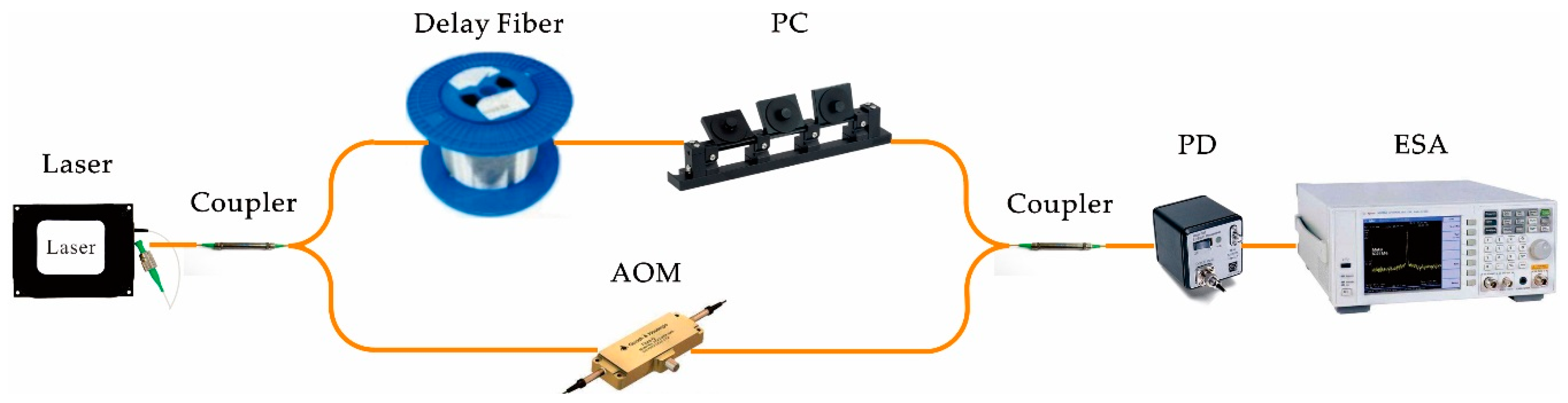
3.1. Experiment Setup for Measuring Laser Linewidth

To measure the linewidth of the utilized lasers, a linewidth measurement setup based on the delayed self-heterodyne interferometer (DSHI) was configured as shown in Figure 6.

The laser output was split into two beams by a 1 × 2 coupler. The upper beam was delayed by a section of single-mode fiber. A polarization controller was used for reducing the polarization mismatch. The lower beam passes through an acoustic optical modulator (AOM) to be frequency shifted by 200 MHz. Finally, the two beams beat in a photodetector through a 3-dB coupler. The electronic signal after PD was acquired and recorded by an electrical spectrum analyzer (ESA). Five lasers with different linewidths were utilized in the experiments.

Table 1. Nominal specifications of the five lasers used in the experiments.

	Model	DFB-LSM-1550-20-PM	Manufacturer
	Wavelength	1550.12 nm
	Nominal linewidth	1.1 MHz
	Max power	20 mw
	Model	KG-DFB-15-M-10-S-FP	Manufacturer
	Wavelength	1550.12 nm
	Nominal linewidth	100 kHz
	Max power	20 mw
	Model	COSF-SC-1550-M	Manufacturer
	Wavelength	1550.12 nm
	Nominal linewidth	10 kHz
	Max power	10 mw
	Model	SDAS-NLW-PL	Manufacturer
	Wavelength	1550.12 nm
	Nominal linewidth	3 kHz
	Max power	17 mw
	Model	Koheras BasiK E15	Manufacturer
	Wavelength	1550.12 nm
	Nominal linewidth	<100 Hz
	Max power	40 mw

gives their nominal specifications.

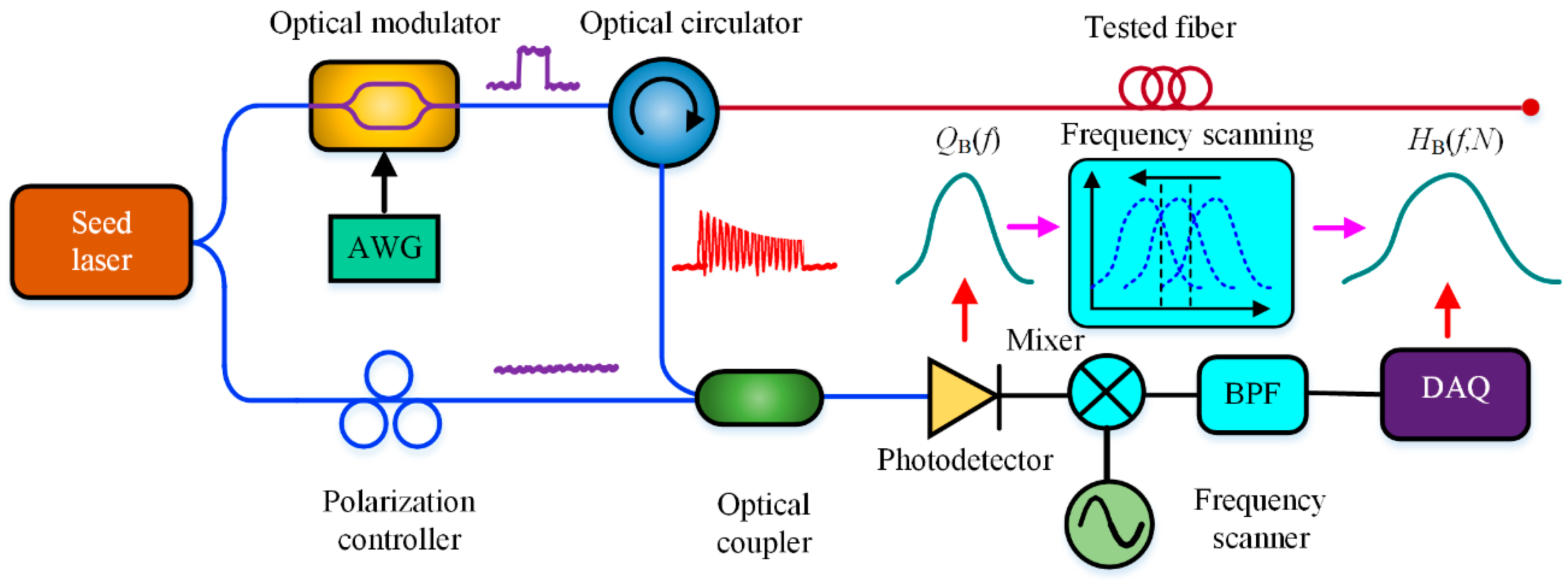
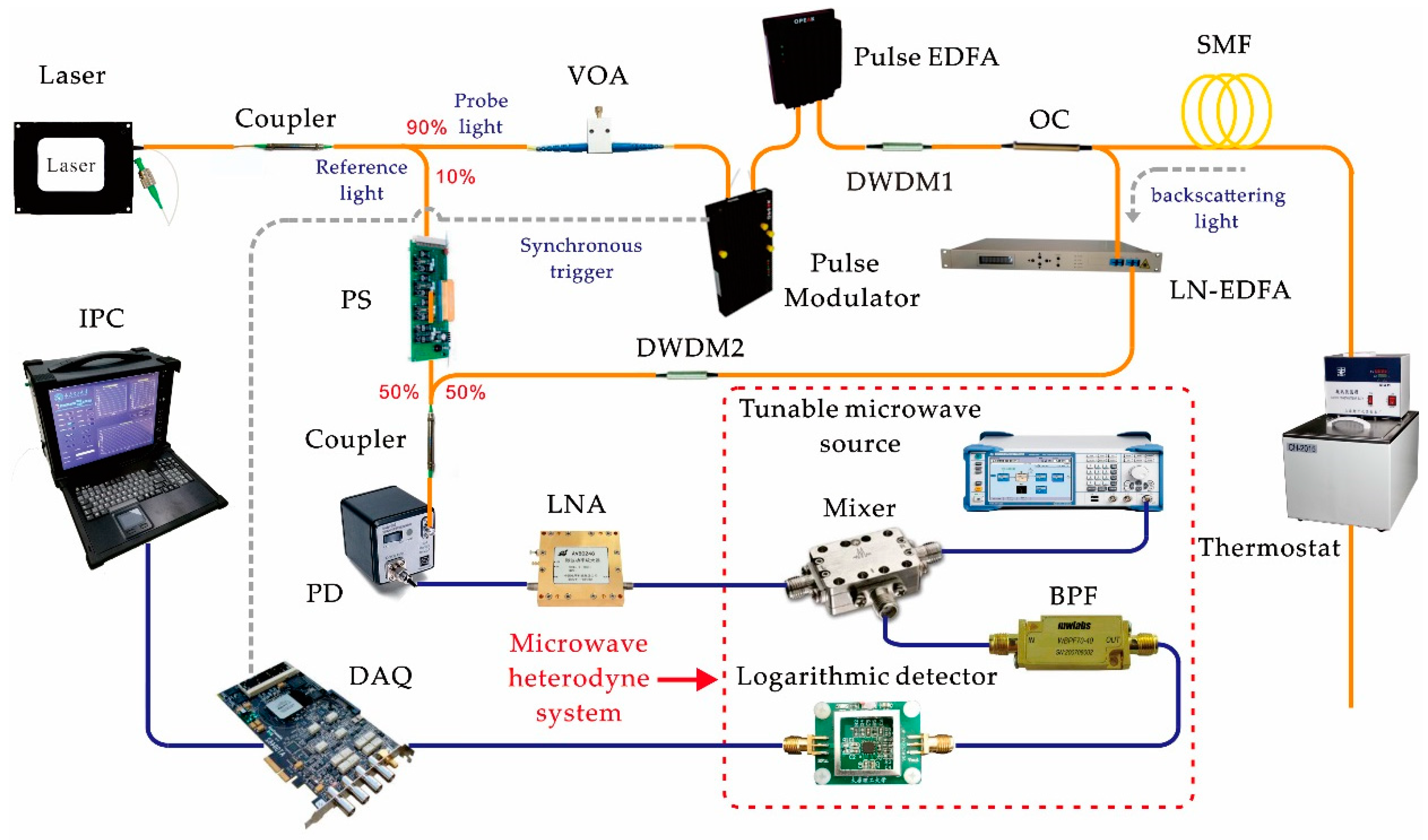
3.2. FS-BOTDR Setup for Measuring BFS

A FS-BOTDR for measuring BFS change arising from temperature was built to verify the influence of the laser linewidth on BFS measurement accuracy, as shown in Figure 7.

The continuous light from the laser was divided into two beams through a 90:10 coupler. The 10% beam as reference light beats with the Brillouin backscattering for coherent heterodyne detection. The polarization scrambler (PS) was for eliminating the polarization noise. The 90% beam was attenuated to the proper power via a variable optical attenuator (VOA) and injected into a pulse modulator for generating probe pulses. The peak power of the probe pulse was amplified by a pulse erbium-doped fiber amplifier (Pulse EDFA) and filtered by a dense wavelength division multiplexer (DWDM1) to remove the amplified spontaneous emission (ASE) noise. Then, the probe pulse was launched into the sensing fiber through an optical circulator (OC). The Brillouin backscattering was amplified by the low-noise EDFA (LN-EDFA), filtered by the DWDM2, and then beats with the reference light in a 13.5-GHz photodetector (PD) through a 50:50 coupler. The beating signal was amplified by an electronic low-noise amplifier (LNA) and connected to a microwave heterodyne system.

In the microwave heterodyne system, the beating signal was mixed with a tunable microwave source to perform frequency scanning, the output frequency of which increased from 11.2 GHz to 11.4 GHz with a fixed frequency internal. The mixed signal was filtered by a BPF with the center frequency of 600 MHz and bandwidth of 87 MHz. The time-domain power trace along the sensing fiber at every scanned frequency obtained by a logarithmic detector and acquired by the data acquisition (DAQ) digitalizer. Every power trace was averaged 2¹³ times. Eventually, the power points obtained at all scanned frequencies were fitted to the Lorentzian profile in an industrial personal computer (IPC), for calculating the BFS distribution along the fiber.

4. Experiment Results and Discussions

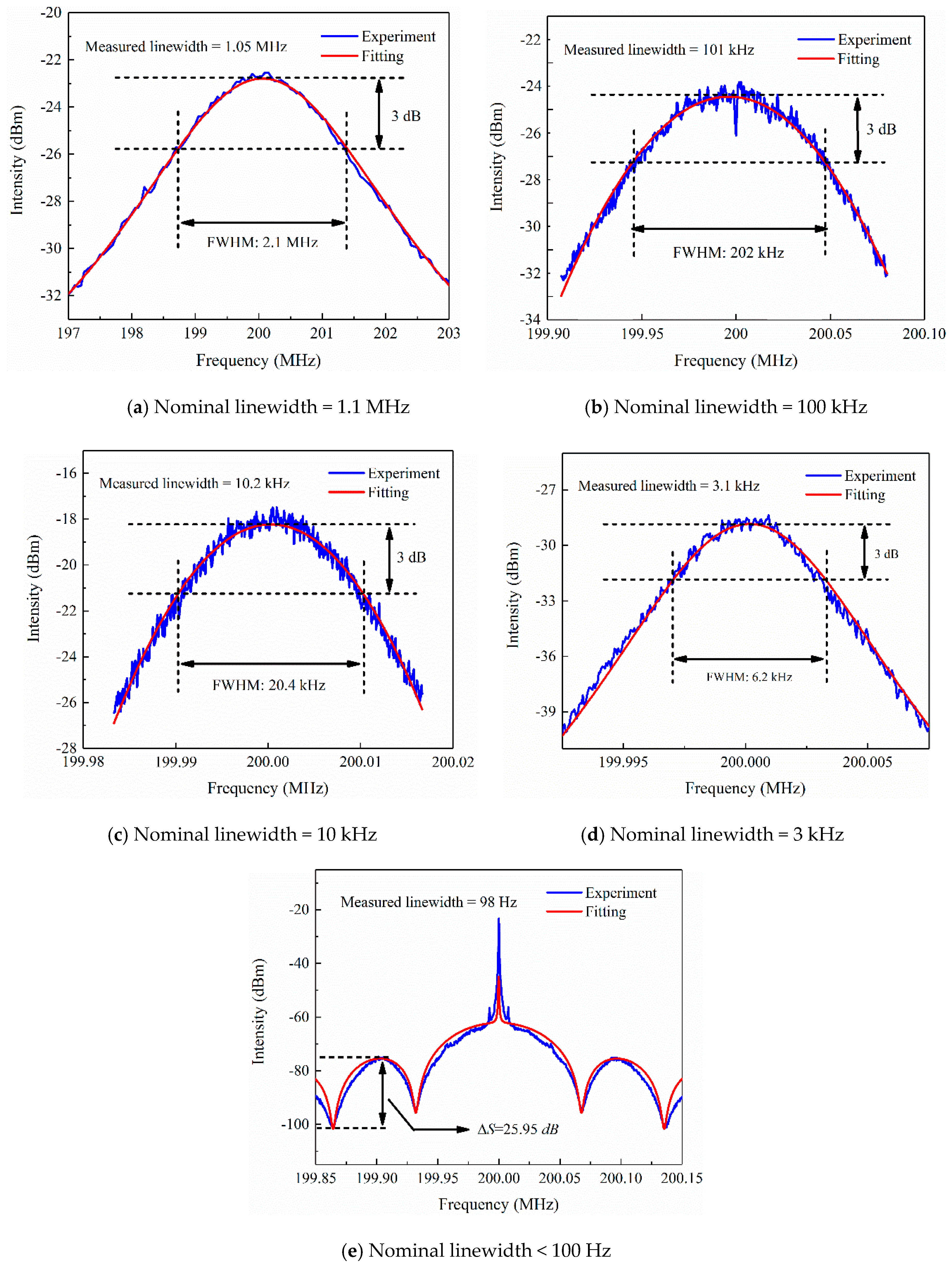
4.1. Measurement of Laser Linewidth

The length of the delay fiber can be settled to 25km for measuring the nominal linewidth from 3 kHz to 1.0 MHz [30], and can be settled to 2950 m for less than 100 Hz [31]. The beating spectrums and fitting results are shown in Figure 8. In Figure 8a–d, the FWHM of the fitted spectrum was twice the laser linewidth, hence the measured linewidths of five lasers were, respectively, 1.05 MHz, 101 kHz, 10.2 kHz, and 3.1k Hz, which were close to the nominal specifications. For the linewidth less than 100 Hz, the accurate measured linewidth was calculated by utilizing the value of ΔS by the amplitude difference comparison of coherent envelope (ADCCE) method (See Appendix B) [31], because the length of the 2950 m delay fiber was much shorter than the coherence length of the measured laser. The accurate linewidth was 98 Hz, as shown in Figure 8e, according to the ADCCE method.

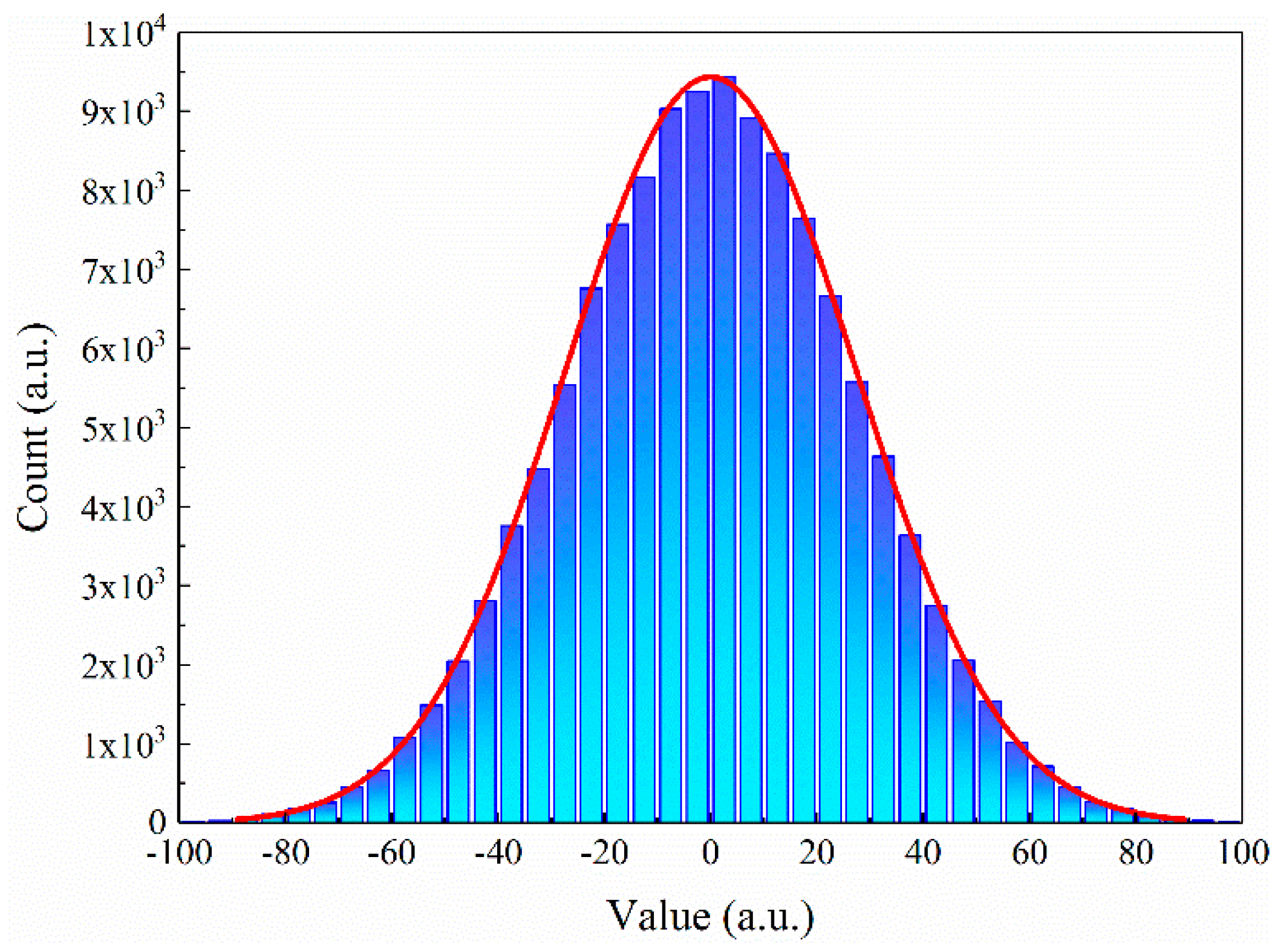
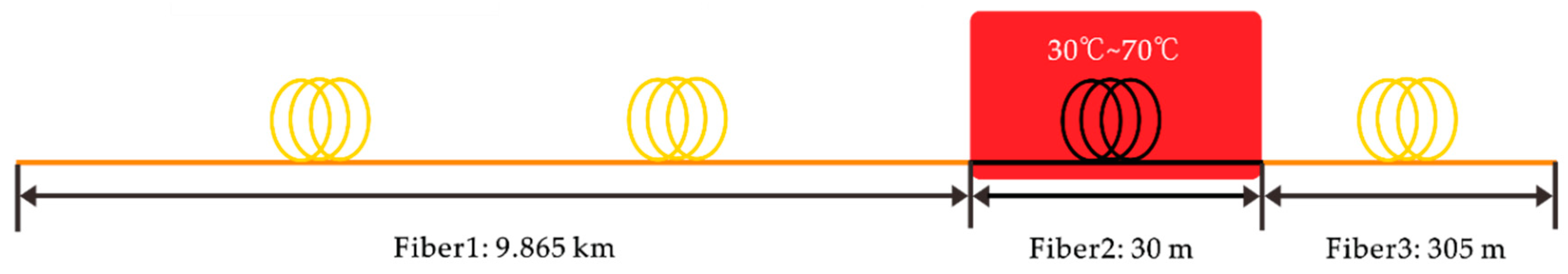
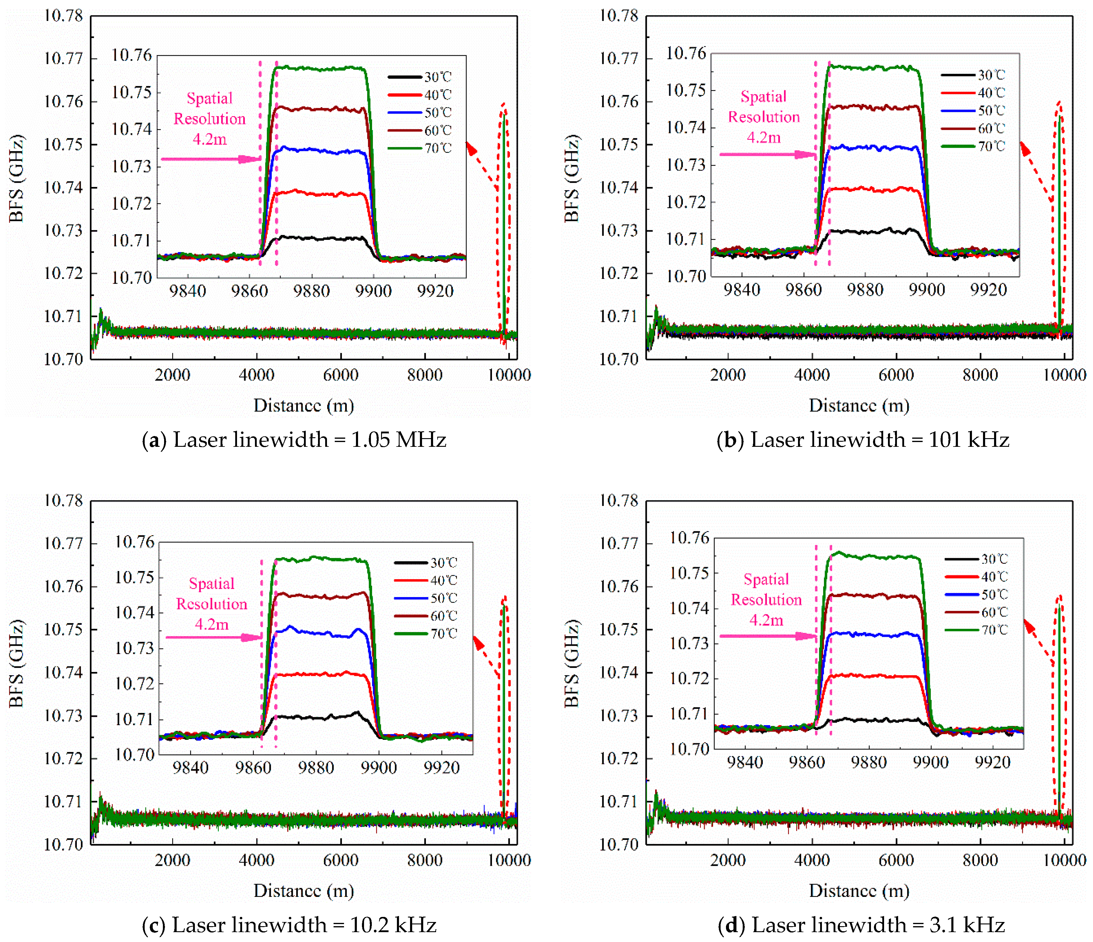
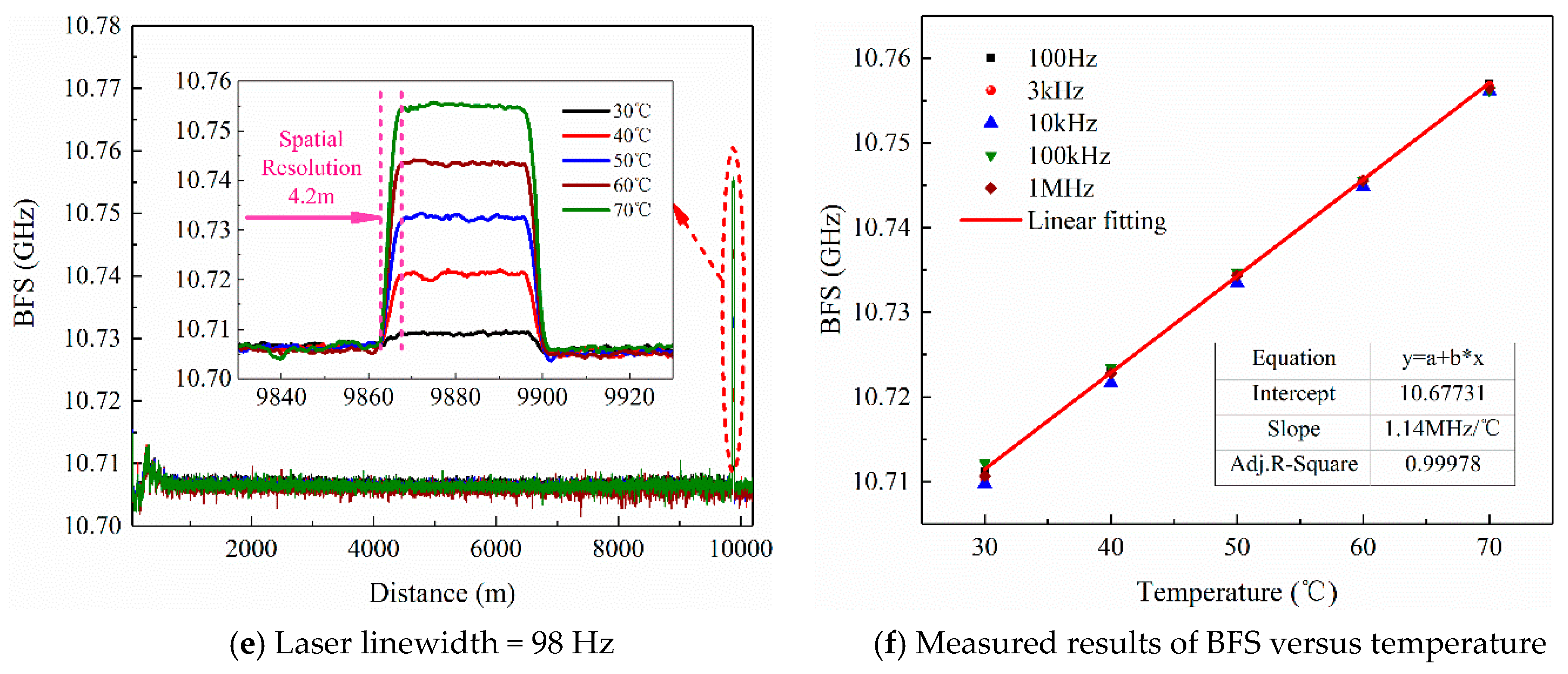
4.2. BFS Distribution Measurement

To verify whether the built FS-BOTDR is capable of measuring the BFS change normally, the temperature measurements were firstly performed utilizing the five lasers mentioned above as the seed source, respectively. Figure 9 gives the configuration of the tested fiber for temperature measurement. The fiber 1 with the length of 9865 m and the fiber 3 with the length of 305 m were placed at room temperature of ~25 °C. The fiber 2 with the length of 30m was placed in a thermostat, the temperature of which was adjusted to change the BFS of fiber 2. As a contrast, the BFS of fiber 1 and fiber 3 were kept nearly constant in the room temperature.

During the experiments, the width of the probe pulse light was set to 42 ns and the peak power was set to 23.09 dBm. The thermostat temperature was sequentially adjusted to 30 °C, 40 °C, 50 °C, 60 °C, and 70 °C, respectively. Then, the BFS distribution measured by five lasers at different temperatures are shown in Figure 10a–e.

From Figure 10a–e, it can be clearly seen that all obtained BFS for fiber 2, which was placed in the thermostat, increased linearly as the temperature increased from 30 °C to 70 °C. As a contrast, the BFS for fiber 1 and fiber 3, which stayed in the room temperature of 25 °C, remained almost constant. Besides, the measured spatial resolution was 4.2 m, which conformed to the pulse width of 42 ns. Figure 10f plots the measured results of BFS versus temperature in detail, and the linear fitting was performed based on the measured data. It shows that the slope coefficient between the temperature and the BFS was 1.14 MHz/°C, neatly coincided with that we reported previously [32]. The adjusted R-square was 0.99978, which indicates a strong linear relationship.

From the above experimental results, it is proven that the built FS-BOTDR setup was capable of measuring the BFS change normally, although utilizing five linewidth-different lasers as the seed light source, respectively. In the following section, further experiments were taken based on this setup to evaluate the influence of the laser linewidth on the BGS spectrum and the BFS accuracy in detail.

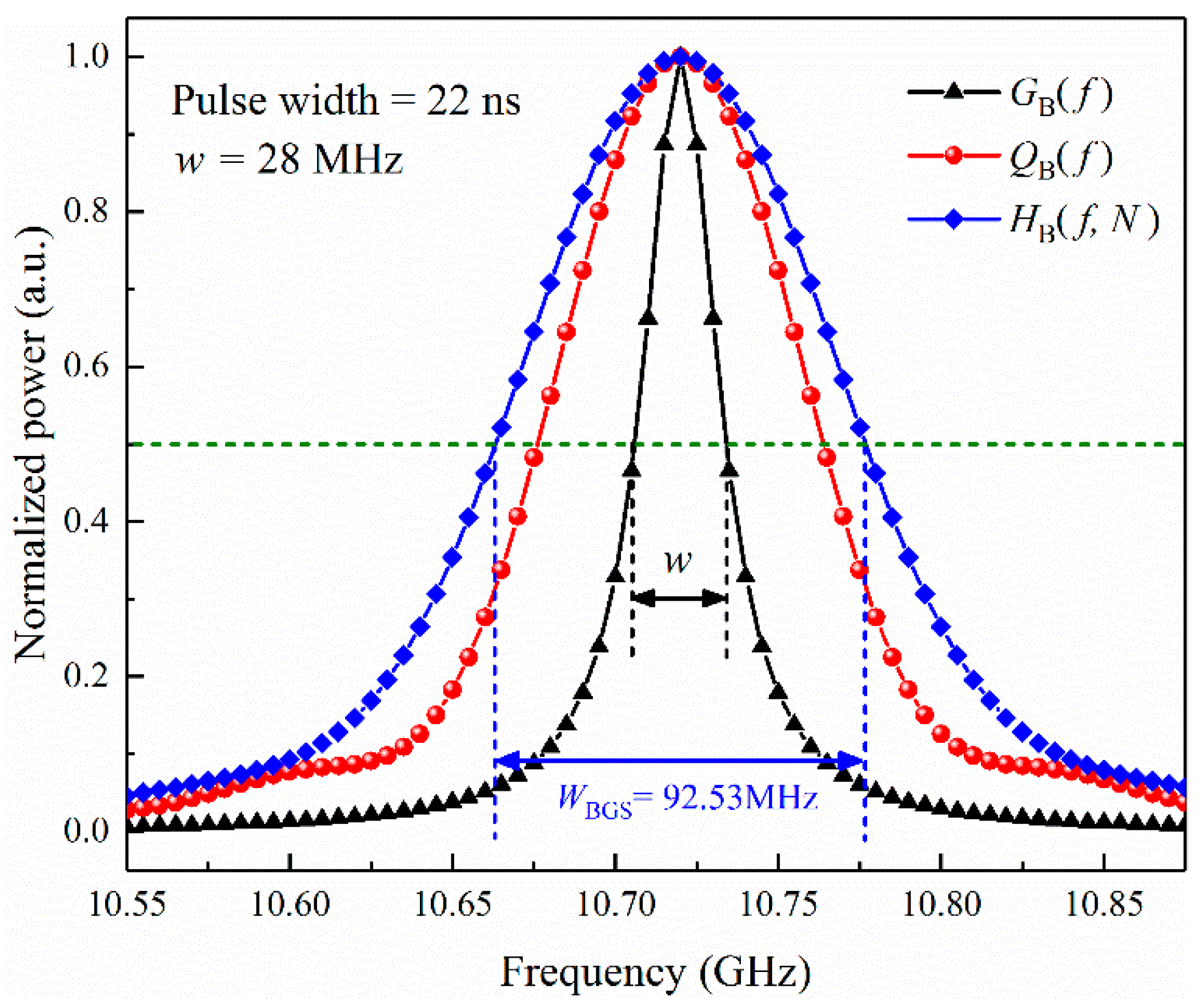
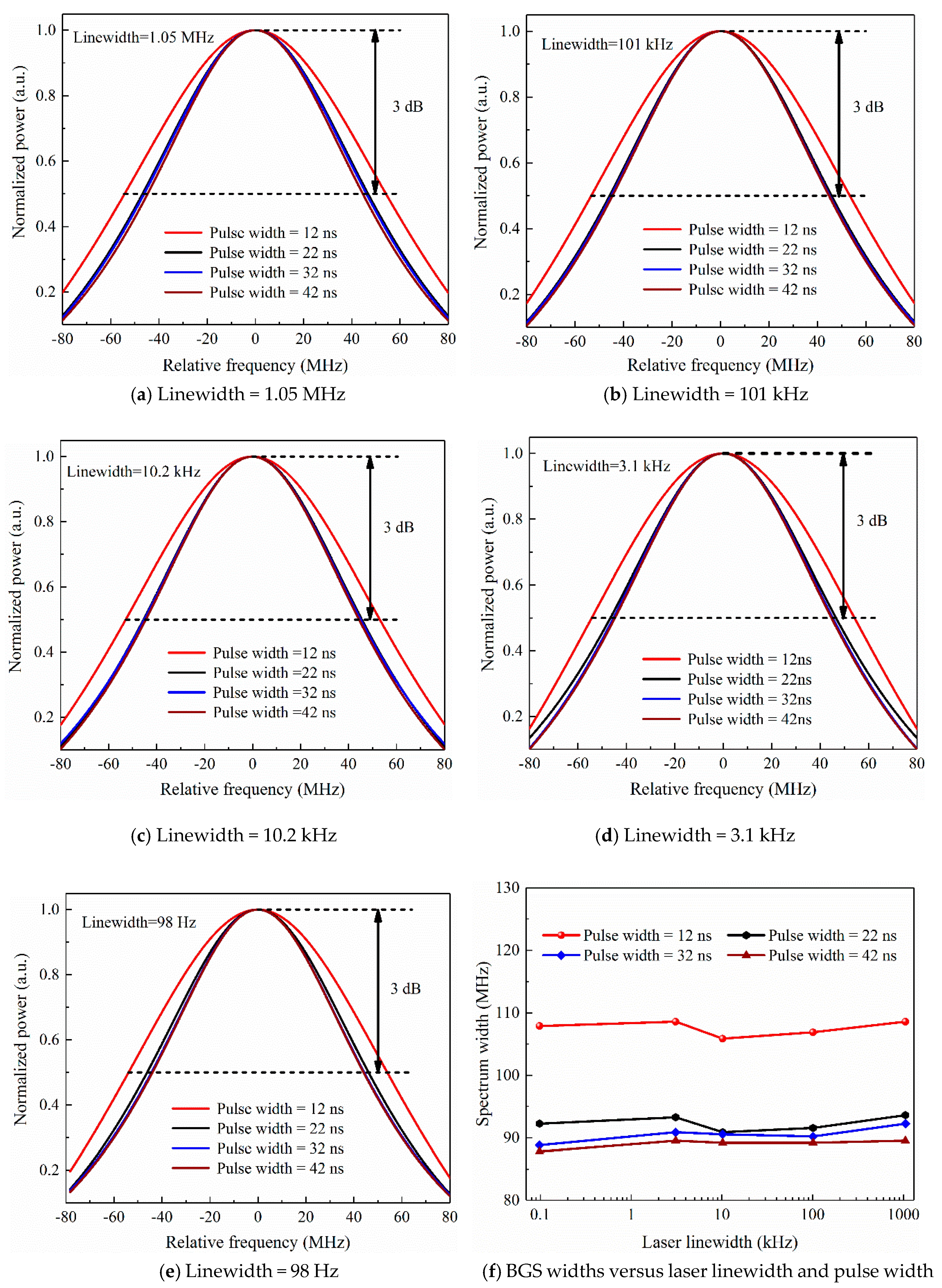
4.3. BGS Width Evaluation

To verify the influence of the laser linewidth on the BGS width, multiple BFS measurements were taken by utilizing the five lasers mentioned above as the seed source, respectively, when the temperature of the thermostat was fixed at 50 °C. The room temperature was kept at a roughly constant temperature of 25 °C. The width of the probe pulse was orderly adjusted to 12 ns, 22 ns, 32 ns, and 42 ns, with the same peak power of 23.09 dBm. For further analysis, we extracted the measured BGSs at 9880 m of tested fiber, the middle of the heated fiber, and fitted them to the Lorentzian profile based on the Levenberg-Marquart algorithm. These BGSs were finally normalized by peak power and are presented in Figure 11a–e, where the relative frequency of the horizontal axis was obtained by f − f_B. The BGS widths versus the laser linewidth is summarily plotted in Figure 11f, when the width of the probe pulse was increased from 12 ns to 42 ns.

From Figure 11f, the BGS width narrowed from ~108 MHz to ~88 MHz as the probe pulse width was increased from 12 ns to 42 ns, which roughly agrees with the theoretical simulations (see Figure 3b, blue line). However, the BGS width showed no distinct tendency as the laser width was broadened from 98 Hz to 1.05 MHz. Hence, it proves that the measured BGS width depended largely on the probe pulse width when the laser linewidth was less than 1MHz, which conformed to the conclusion reported previously [23].

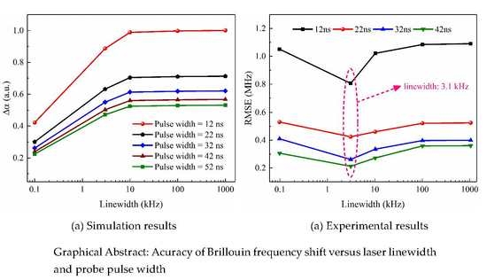
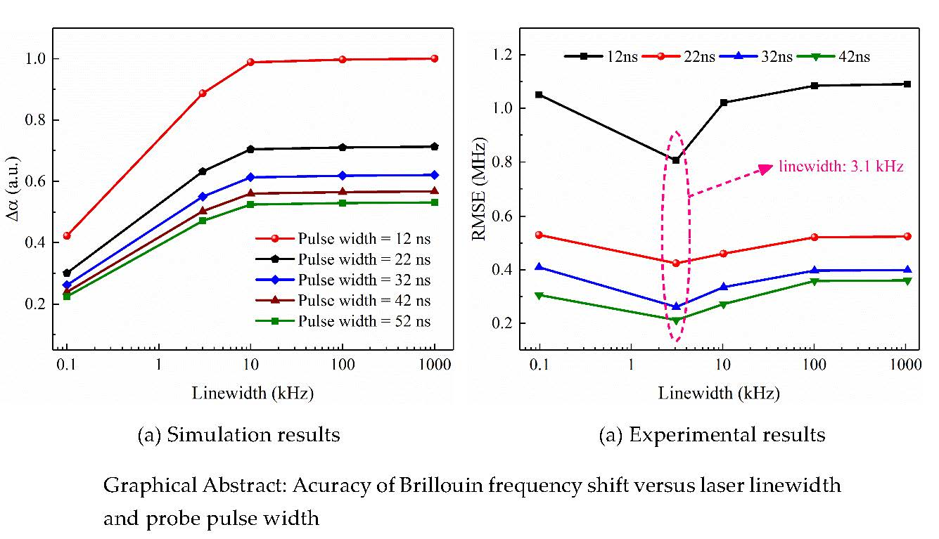
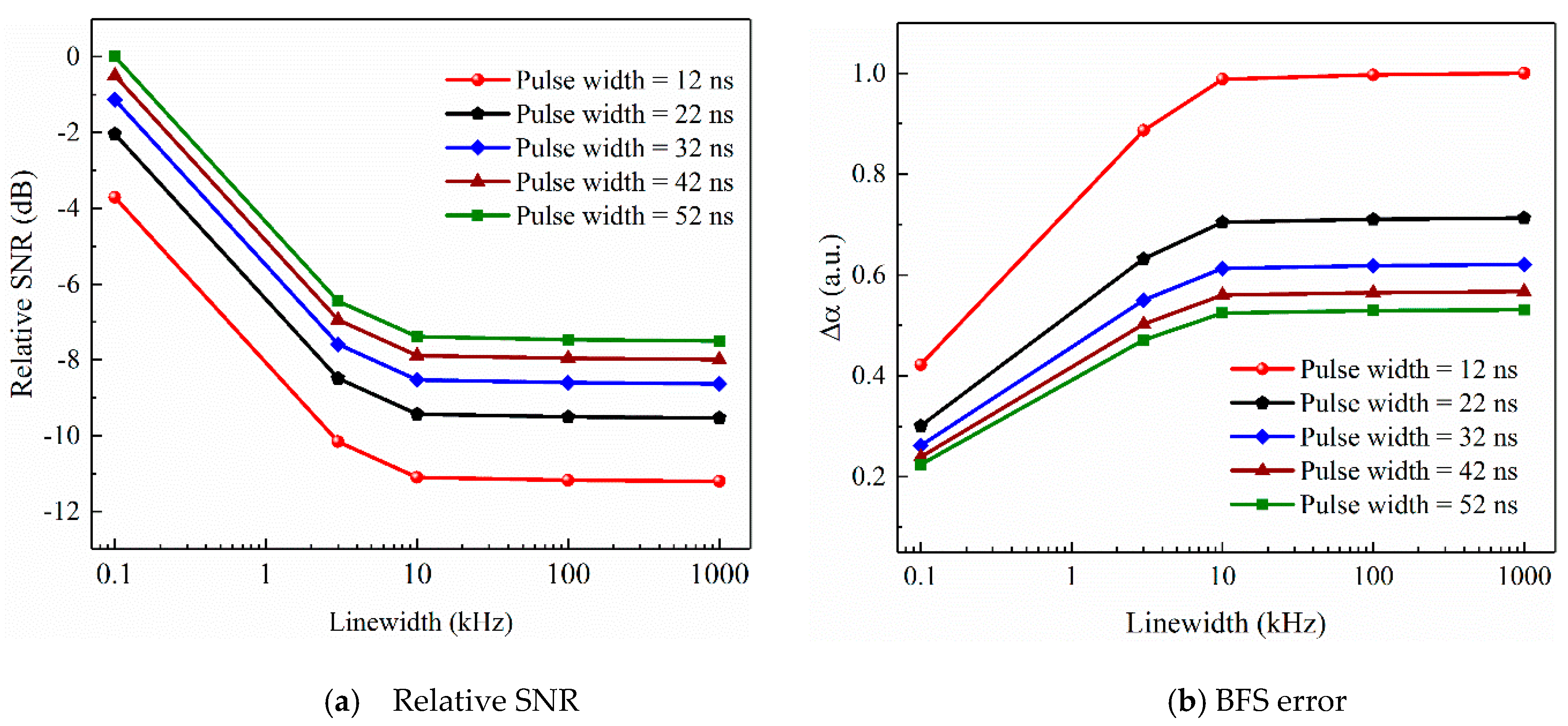
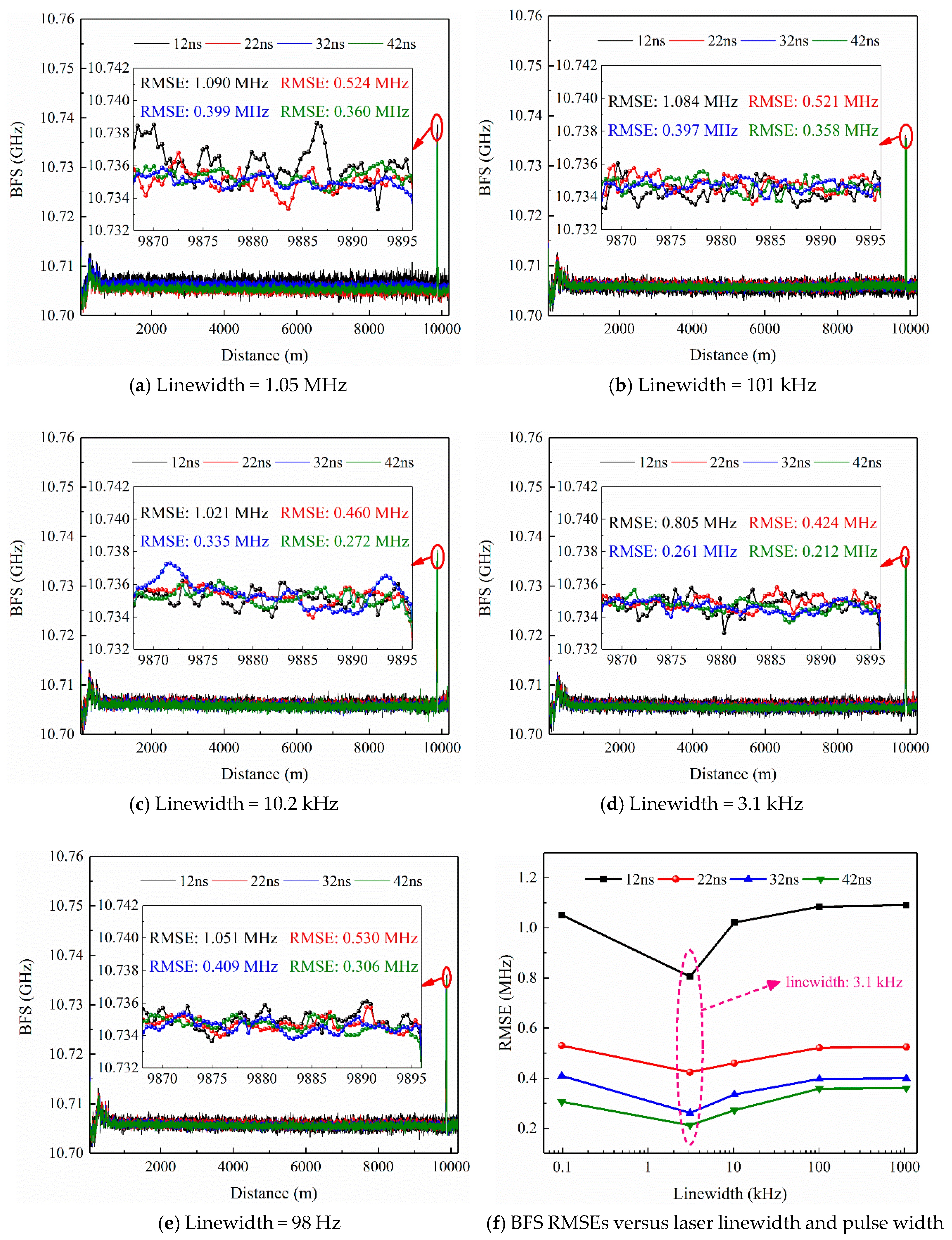
4.4. BFS Accuracy Evaluation

For further evaluating the influence of the laser linewidth on the BFS accuracy, the measured BFS over the heated fiber were specially extracted and are shown in the inset of Figure 12a–e, eliminating the rise and fall edge of BFS change. The root-mean-square errors (RMSEs) of the extracted BFS distribution were calculated and plotted versus the laser linewidth and pulse width, as shown in Figure 12f.

From Figure 12f, it can be seen that the RMSE of BFS was related with both the laser linewidth and the probe pulse width. It decreased obviously when the pulse width was extended from 12 ns to 42 ns. When the pulse width was fixed, the RMSE of BFS decreased with the laser linewidth narrowing from 1.05 MHz to 3.1 kHz, which was in good agreement with the numerical simulations. However, it unexpectedly increased as the laser linewidth narrowed from 3.1 kHz to 98 Hz, which was inconsistent with the simulation results. We contribute this exception to the coherent Rayleigh noise (CRN). The CRN increases sharply as the laser linewidth becomes narrower [33]. Additionally, it has been proven that the CRN cannot be reduced by signal averaging [34]. Hence, the accuracy of BOTDR will decrease once the linewidth of the seed laser becomes narrow to a certain value, such as 98 Hz in this paper, because the extremely-narrow laser linewidth enhances the CRN largely and further results in sharp SNR deterioration of the BOTDR.

Based on the above analysis, it was demonstrated that the BFS accuracy improves when the laser linewidth narrows. However, the BFS accuracy will deteriorate when the laser linewidth is so narrow that the CRN is enhanced sharply. The measured results of BFS RMSE and BGS width (W_BGS) by respectively utilizing five different-linewidth lasers as the seed source are summarily listed in

Table 2. Summary list of measured results in experiments.

Laser Linewidth	Peak Power	12 ns		22 ns		32 ns		42ns
		RMSE	WBGS	RMSE	WBGS	RMSE	WBGS	RMSE	WBGS
------	dBm	MHz	MHz	MHz	MHz	MHz	MHz	MHz	MHz
1.05 MHz	23.09	1.090	108.6	0.524	93.6	0.399	92.2	0.360	89.5
101 kHz	23.09	1.084	106.9	0.521	91.6	0.397	90.2	0.358	89.2
10.2 kHz	23.09	1.021	105.8	0.460	90.9	0.335	90.5	0.272	89.2
3.1 kHz	23.09	0.805	108.6	0.424	93.3	0.261	90.9	0.212	89.5
98 Hz	23.09	1.051	107.9	0.531	92.2	0.409	88.8	0.306	89.8

, where the probe pulse width was 12 ns, 22 ns, 32 ns, and 42 ns with the same peak power of 23.09 dBm.

5. Conclusions

In this paper, the influence of the laser linewidth on BFS accuracy in the FS-BOTDR was analyzed. The BGS broadening effect and the SNR of the FS-BOTDR was numerically simulated by taking phase fluctuation as the major noise contribution. The simulation results presented that the RMSE of BFS decreases when the laser linewidth narrows. In the experiments, we utilized five different lasers as the seed source, respectively, to measure the BFS change. The linewidth of the five lasers were, correspondingly, 1.05 MHz, 101 kHz, 10.2 kHz, 3.1 kHz, and 98 Hz. As the pulse width increased from 12 ns to 42 ns, the BGS width and BFS accuracy were further evaluated and discussed in detail.

The experimental results indicate that the BFS accuracy improves with the laser linewidth narrowing. However, the BFS accuracy will deteriorate when the laser linewidth decreases to a certain value, such as 98 Hz in this paper. The exception may arise from the increasing CRN related closely with the narrowing linewidth. Therefore, how the CRN affects the BFS accuracy needs to be further theoretically explained and experimentally verified in future, if an extremely-narrow-linewidth laser is utilized in a FS-BOTDR. The results in this paper will be helpful to choose an appropriate laser for BOTDR, and provide potential techniques for improving the measurement accuracy of temperature or strain based BOTDR.

References

1. Kurashima, T.; Horiguchi, T.; Izumita, H.; Furukawa, S.; Koyamada, Y. Brillouin optical-fiber time domain reflectometry. IEICE Trans. Commun. 1993, E76-B, 382–390. [Google Scholar]
2. Geng, J.; Staines, S.; Blake, M.; Jiang, S. Distributed fiber temperature and strain sensor using coherent radio-frequency detection of spontaneous Brillouin scattering. Appl Opt. 2007, 46, 5928–5932. [Google Scholar] [CrossRef] [PubMed]
3. Li, A.; Wang, Y.; Hu, Q.; Che, D.; Chen, X.; Shieh, W. Measurement of distributed mode coupling in a few-mode fiber using a reconfigurable Brillouin OTDR. Opt. Lett. 2014, 39, 6418–6421. [Google Scholar] [CrossRef] [PubMed]
4. Hong, C.; Zhang, Y.; Li, G.; Zhang, M.; Liu, Z. Recent progress of using Brillouin distributed fiber optic sensors for geotechnical health monitoring. Sens. Actuators A 2017, 258, 131–145. [Google Scholar] [CrossRef]
5. Soto, M.A.; Bolognini, G.; Di Pasquale, F. Enhanced simultaneous distributed strain and temperature fiber sensor employing spontaneous Brillouin scattering and optical pulse coding. IEEE Photonic Technol. Lett. 2009, 21, 450–452. [Google Scholar] [CrossRef]
6. Kim, S.; Kwon, H.; Yang, I.; Lee, S.; Kim, J.; Kang, S. Performance of a distributed simultaneous strain and temperature sensor based on a Fabry-Perot laser diode and a dual-stage FBG optical demultiplexer. Sensors 2013, 13, 15452–15464. [Google Scholar] [CrossRef] [PubMed]
7. Webb, G.T.; Vardanega, P.J.; Hoult, N.A.; Fidler, P.R.A.; Bennett, P.J.; Middleton, C.R. Analysis of fiber-optic strain-monitoring data from a prestressed concrete bridge. J. Bridge Eng. 2017, 22, 05017002. [Google Scholar] [CrossRef]
8. Moffat, R.; Sotomayor, J.; Beltrán, J.F. Estimating tunnel wall displacements using a simple sensor based on a brillouin optical time domain reflectometer apparatus. Int. J. Rock Mech. Min. Sci. 2015, 75, 233–243. [Google Scholar] [CrossRef]
9. Hao, Y.; Cao, Y.; Ye, Q.; Cai, H.; Qu, R. On-line temperature monitoring in power transmission lines based on Brillouin optical time domain reflectometry. Optik 2015, 126, 2180–2183. [Google Scholar] [CrossRef]
10. Naruse, H.; Uehara, H.; Deguchi, T.; Fujihashi, K.; Onishi, M.; Espinoza, R.; Guzman, C.; Pardo, C.; Ortega, C.; Pinto, M. Application of a distributed fibre optic strain sensing system to monitoring changes in the state of an underground mine. Meas. Sci. Technol. 2007, 18, 3202–3210. [Google Scholar] [CrossRef]
11. Maughan, S.M.; Kee, H.H.; Newson, T.P. 57-km single-ended spontaneous Brillouin-based distributed fiber temperature sensor using microwave coherent detection. Opt. Lett. 2001, 26, 331–333. [Google Scholar] [CrossRef] [PubMed]
12. Yao, Y.; Lu, Y.; Zhang, X.; Wang, F.; Wang, R. Reducing trade-off between spatial resolution and frequency accuracy in BOTDR using Cohen's Class signal processing method. IEEE Photonic Technol. Lett. 2012, 24, 1337–1339. [Google Scholar] [CrossRef]
13. Wang, F.; Zhan, W.; Lu, Y.; Yan, Z.; Zhang, X. Determining the change of Brillouin frequency shift by using the similarity matching method. J. Lightwave Technol. 2015, 33, 4101–4108. [Google Scholar] [CrossRef]
14. Zheng, H.; Fang, Z.; Wang, Z.; Lu, B.; Cao, Y.; Ye, Q.; Qu, R.; Cai, H. Brillouin frequency shift of fiber distributed sensors extracted from noisy signals by quadratic fitting. Sensors 2018, 18, 409. [Google Scholar] [CrossRef] [PubMed]
15. Hao, Y.; Ye, Q.; Pan, Z.; Cai, H.; Qu, R. Analysis of spontaneous Brillouin scattering spectrum for different modulated pulse shape. Optik 2013, 124, 2417–2420. [Google Scholar] [CrossRef]
16. Hao, Y.; Ye, Q.; Pan, Z.; Cai, H.; Qu, R.; Yang, Z. Effects of modulated pulse format on spontaneous Brillouin scattering spectrum and BOTDR sensing system. Opt. Laser Technol. 2013, 46, 37–41. [Google Scholar] [CrossRef]
17. Wang, F.; Zhu, C.; Cao, C.; Zhang, X. Enhancing the performance of BOTDR based on the combination of FFT technique and complementary coding. Opt. Express 2017, 25, 3504–3513. [Google Scholar] [CrossRef]
18. Hao, Y.; Ye, Q.; Pan, Z.; Cai, H.; Qu, R. Digital coherent detection research on Brillouin optical time domain reflectometry with simplex pulse codes. Chin. Phys. B 2014, 23. [Google Scholar] [CrossRef]
19. Lu, Y.; Yao, Y.; Zhao, X.; Wang, F.; Zhang, X. Influence of non-perfect extinction ratio of electro-optic modulator on signal-to-noise ratio of BOTDR. Opt. Commun. 2013, 297, 48–54. [Google Scholar] [CrossRef]
20. Zhang, Y.; Wu, X.; Ying, Z.; Zhang, X. Performance improvement for long-range BOTDR sensing system based on high extinction ratio modulator. Electron. Lett 2014, 50, 1014–1016. [Google Scholar] [CrossRef]
21. Lalam, N.; Ng, W.P.; Dai, X.; Wu, Q.; Fu, Y.Q. Performance improvement of Brillouin ring laser based BOTDR system employing a wavelength diversity technique. J. Lightwave Technol. 2018, 36, 1084–1090. [Google Scholar] [CrossRef]
22. Li, C.; Lu, Y.; Zhang, X.; Wang, F. SNR enhancement in Brillouin optical time domain reflectometer using multi-wavelength coherent detection. Electron. Lett 2012, 48, 1139–1141. [Google Scholar] [CrossRef]
23. Hao, Y.; Ye, Q.; Pan, Z.; Cai, H.; Qu, R. Influence of laser linewidth on performance of Brillouin optical time domain reflectometry. Chin. Phys. B 2013, 22. [Google Scholar] [CrossRef]
24. Naruse, H.; Tateda, M. Trade-off between the spatial and the frequency resolutions in measuring the power spectrum of the Brillouin backscattered light in an optical fiber. Appl. Opt. 1999, 38, 6516–6521. [Google Scholar] [CrossRef] [PubMed]
25. Zheng, Z.; Zhao, C.; Zhang, H.; Yang, S.; Zhang, D.; Yang, H.; Liu, J. Phase noise reduction by using dual-frequency laser in coherent detection. Opt. Laser Technol. 2016, 80, 169–175. [Google Scholar] [CrossRef]
26. Motil, A.; Bergman, A.; Tur, M. State of the art of Brillouin fiber-optic distributed sensing. Opt. Laser Technol. 2016, 78, 81–103. [Google Scholar] [CrossRef]
27. Nikles, M.; Thevenaz, L.; Robert, P.A. Brillouin gain spectrum characterization in single-mode optical fibers. J. Lightwave Technol. 1997, 15, 1842–1851. [Google Scholar] [CrossRef] [Green Version]
28. Hui, R.; O'Sullivan, M. Fiber Optic Measurement Techniques; Elsevier Academic Press: Burlington, MA, USA, 2009; pp. 196–199. [Google Scholar]
29. Du, Z.; Lu, L.; Wang, B.; Jiang, C. Effect of laser diode phase noise on coherent sensing systems. In Proceedings of the 13th International Conference on Advanced Laser Technologies, Tianjin, China, 3–6 September 2005. [Google Scholar] [CrossRef]
30. NKT Photonics. Laser Spectral Linewidth. Available online: http://www.sevensix.co.jp/wordpress/wp-content/uploads/2017/07/Linewidth-Application-Note-Version-1-1-October-2013.pdf (accessed on 9 December 2018).
31. Huang, S.; Zhu, T.; Cao, Z.; Liu, M.; Deng, M.; Liu, J.; Li, X. Laser linewidth measurement based on amplitude difference comparison of coherent envelope. IEEE Photonic Technol. Lett. 2016, 28, 759–762. [Google Scholar] [CrossRef]
32. Liu, R.; Zhang, M.; Zhang, J.; Liu, Y.; Jin, B.; Bai, Q.; Li, Z. Temperature measurement accuracy enhancement in the Brillouin optical time domain reflectometry system using the sideband of Brillouin gain spectrum demodulation. Acta Phys. Sin. 2016, 65. [Google Scholar] [CrossRef]
33. Reshak, A.H.; Shahimin, M.M.; Murad, S.A.Z.; Azizan, S. Simulation of Brillouin and Rayleigh scattering in distributed fibre optic for temperature and strain sensing application. Sens. Actuators A 2013, 190, 191–196. [Google Scholar] [CrossRef]
34. De Souza, K. Significance of coherent rayleigh noise in fibre-optic distributed temperature sensing based on spontaneous Brillouin scattering. Meas. Sci. Technol. 2006, 17, 1065–1069. [Google Scholar] [CrossRef]
Figure 1. Schematic diagram of frequency-scanning BOTDR (FS-BOTDR) with coherent heterodyne detection: AWG = Arbitrary Waveform Generator; BPF = Band-pass Filter; DAQ = Data Acquisition.
Applsci 09 00058 g001
Figure 2. Numerical simulation of the broadening effect of Brillouin gain spectrum (BGS) in FS-BOTDR: GB(f) is the original BGS for the continuous light; QB(f) is the BGS for the pulse light with a width of 22 ns; HB(f, N) is the final measured BGS through the frequency-scanning process when the width of the probe pulse is 22 ns.
Applsci 09 00058 g002
Figure 3. Numerical simulation results: (a) Profiles of HB(f, N) under different probe pulse widths; (b) spectrum width and relative power versus probe pulse width.
Applsci 09 00058 g003
Figure 4. Histogram of Δφ utilized in the simulation when Δf = 1.05 MHz and ΔL = 20 km.
Applsci 09 00058 g004
Figure 5. Numerical simulation results versus laser linewidth under different pulse widths: (a). Relative signal-to-noise ratio (SNR); (b). BFS accuracy. Model parameters utilized for simulations are listed in Table A1.
Applsci 09 00058 g005
Figure 6. Delayed self-heterodyne interferometer to measure the laser linewidth.
Applsci 09 00058 g006
Figure 7. FS-BOTDR setup for temperature sensing.
Applsci 09 00058 g007
Figure 8. Linewidth measurement results of five lasers, of which the nominal linewidth are respectively: (a). 1.1 MHz; (b). 100 kHz; (c). 10 kHz; (d). 3 kHz; (e). <100 Hz.
Applsci 09 00058 g008
Figure 9. Configuration of the tested fiber for temperature measurement.
Applsci 09 00058 g009
Figure 10. BFS distributions at different temperatures when the laser linewidth is: (a) 1.05 MHz; (b) 101 kHz; (c) 10.2 kHz; (d) 3.1 kHz; and (e) 98 Hz. (f) Measured results of BFS versus temperature.
Applsci 09 00058 g010aApplsci 09 00058 g010b
Figure 11. Normalized BGS extracted at the middle of the heated fiber when the laser linewidth is: (a) 1.05 MHz, (b) 101 kHz, (c) 10.2 kHz, (d) 3.1 kHz, and (e) 98 Hz; (f) BGS widths versus laser linewidth and pulse width.
Applsci 09 00058 g011
Figure 12. Measured BFS distribution when the linewidth is: (a) 1.05 MHz, (b) 101 kHz, (c) 10.2 kHz, (d) 3.1 kHz, and (e) 98 Hz; (f) BFS root-mean-square errors (RMSEs) versus laser linewidth and probe pulse width.
Applsci 09 00058 g012