Semi-Analytic Monte Carlo Model for Oceanographic Lidar Systems: Lookup Table Method Used for Randomly Choosing Scattering Angles

Featured Application

A lookup table method is proposed for solving complicated or even unsolvable inverse cumulative distribution function of scattering phase function.

Abstract

Monte Carlo (MC) is a significant technique for finding the radiative transfer equation (RTE) solution. Nowadays, the Henyey-Greenstein (HG) scattering phase function (spf) has been widely used in most studies during the core procedure of randomly choosing scattering angles in oceanographic lidar MC simulations. However, the HG phase function does not work well at small or large scattering angles. Other spfs work well, e.g., Fournier-Forand phase function (FF); however, solving the cumulative distribution function (cdf) of the scattering phase function (even if possible) would result in a complicated formula. To avoid the above-mentioned problems, we present a semi-analytic MC radiative transfer model in this paper, which uses the cdf equation to build up a lookup table (LUT) of $\psi$ vs. $P_{\Psi }(\psi )$ to determine scattering angles for various spfs (e.g., FF, Petzold measured particle phase function, and so on). Moreover, a lidar geometric model for analytically estimating the probability of photon scatter back to a remote receiver was developed; in particular, inhomogeneous layers are divided into voxels with different optical properties; therefore, it is useful for inhomogeneous water. First, the simulations between the inverse function method for HG cdf and the LUT method for FF cdf were compared. Then, multiple scattering and wind-driven sea surface condition effects were studied. Finally, we compared our simulation results with measurements of airborne lidar. The mean relative errors between simulation and measurements in inhomogeneous water are within 14% for the LUT method and within 22% for the inverse cdf (ICDF) method. The results suggest feasibility and effectiveness of our simulation model.

1. Introduction

Often used to solve the radiative transfer equation (RTE) of oceanographic lidar, Monte Carlo (MC) techniques refer to the algorithms that use probability theory and random numbers to simulate the fates of numerous photons propagating through sea water. The strengths of MC techniques are that they are conceptually simple, which require fewer simplifying approximations, and can be used for finding complicated 3D RTE solutions [1]. In recent years, MC simulation methods have been widely used in lidar propagation in ocean water. Peng-Wang et al. [2,3] developed a three-dimensional vector radiative transfer MC method for light propagation in atmosphere–ocean systems, which provides complete information about radiative coupling between different regions of the system. Ramella-Roman et al. [4,5] presented three MC programs of polarized light transport into scattering media; comparison between MC runs and Adding Doubling program yielded less than 1% error. Berrocal et al. [6] investigated scattering and multiple scattering of a typical laser beam in a turbid environment and obtained good agreement between experimental measurements and results from MC simulations. Gordon [7] studied multiple scattering effects by solving the RTE via MC techniques. The effective attenuation coefficient of this exponential decay is found to be strongly dependent on the parameters of the lidar system and on the optical properties of the water. Poole et al. [8] described a semi-analytic MC radiative transfer model (SALMON), which is particularly well-suited for addressing oceanographic lidar systems. It is based on the method of expected values in which an analytical estimate is made of the probability of collection by a remote receiver of scattered or emitted photons at appropriate points in the stochastically constructed underwater photon trajectory. Chen et al. [9] also developed a semi-analytic MC radiative transfer model to study laser propagation in inhomogeneous sea water within the subsurface plankton layer. Besides, there are many other MC studies for simulating photons propagating in a scattering medium [10,11,12,13].

The probability density function (pdf) for a random variable that can have values only between 0 and 1 is fundamental to MC simulation. Scattering phase function (spf) can be interpreted as a pdf: $\tilde{\beta }(\psi )\sin (\psi )$. The Henyey-Greenstein (HG) spf [14] has been widely used in many studies. The HG phase function, however, does not work well at small or large scattering angles. Though other spfs work well, e.g., Fournier-Forand phase function (FF) [15], solving cumulative distribution function (cdf) of spf $P_{\Psi }(\psi )$ as Equation 1 for scattering angle $\psi$ (even if possible), namely inverse cdf (ICDF), would give a complicated formula. Besides, in almost all of these studies, they assume the water is optically vertical homogeneous; a few studies focus on simulating light propagation in inhomogeneous water. For some use cases there is a need to extend and improve existing MC methods to apply to inhomogeneous water, for instance, the ocean with subsurface chlorophyll maximum layer.

$$P_{\Psi }(\psi )=2\pi {\displaystyle \underset{0}{\overset{\psi }{\int }}\tilde{\beta }({\psi }^{\prime })\sin {\psi }^{\prime }d{\psi }^{\prime }}$$

(1)

This study introduces an improved semi-analytic MC radiative transfer model based on the lookup table (LUT) method and an analytically lidar geometric model to describe photons scattering event for oceanographic lidar systems. The new model presented in this study is based on a lidar geometric model for analytically estimating the probability of photon scatter back to a remote receiver, and inhomogeneous layers are divided into voxels with different optical properties with a resolution as high as 0.11 m. The LUT method is used for solving complicated or even unsolvable inverse cumulative distribution function of various spfs. Multiple scattering and wind-driven sea surface condition effects are also studied. Finally, we compared our simulation results with measurements of airborne lidar.

2. Theory and Modeling

2.1. Determining Photon-Free Path Length in Inhomogeneous Water

Detailed MC simulation for light propagating in sea water requires random determination of photon path length, photon scattering angle, and reflection or transmission at sea surface or bottom boundaries [16]. Most existing MC simulation methods assume that sea water is optically homogeneous, while true sea water is sometimes optically vertical inhomogeneous. It should be noted that “inhomogeneous” water in this study mainly means that vertical optical properties of the water are inhomogeneous. In order to simulate optically inhomogeneous sea water, inhomogeneous layers are divided into voxels with different optical properties. We allow $\alpha (\mathrm{z})$ and $b(\mathrm{z})$ vary with depth $\mathrm{z}$ in this study, where $\alpha (\mathrm{z})$ and $b(\mathrm{z})$ are sea water absorption and scattering coefficient at the depth of $\mathrm{z}$, respectively. Therefore, a series of photon path lengths at different depths are generated as follows:

$$s=\frac{-\ln (\Re )}{c(\mathrm{z})}$$

(2)

where $\Re$ is a series of random numbers, which follow uniform distribution over the interval $[0,1]$, and $c(\mathrm{z})$ is sea water attenuation coefficient, which is the sum of $\alpha (\mathrm{z})$ and $b(\mathrm{z})$. In the case of homogeneous water, the average distance that a photon travels is $\frac{1}{c}$.

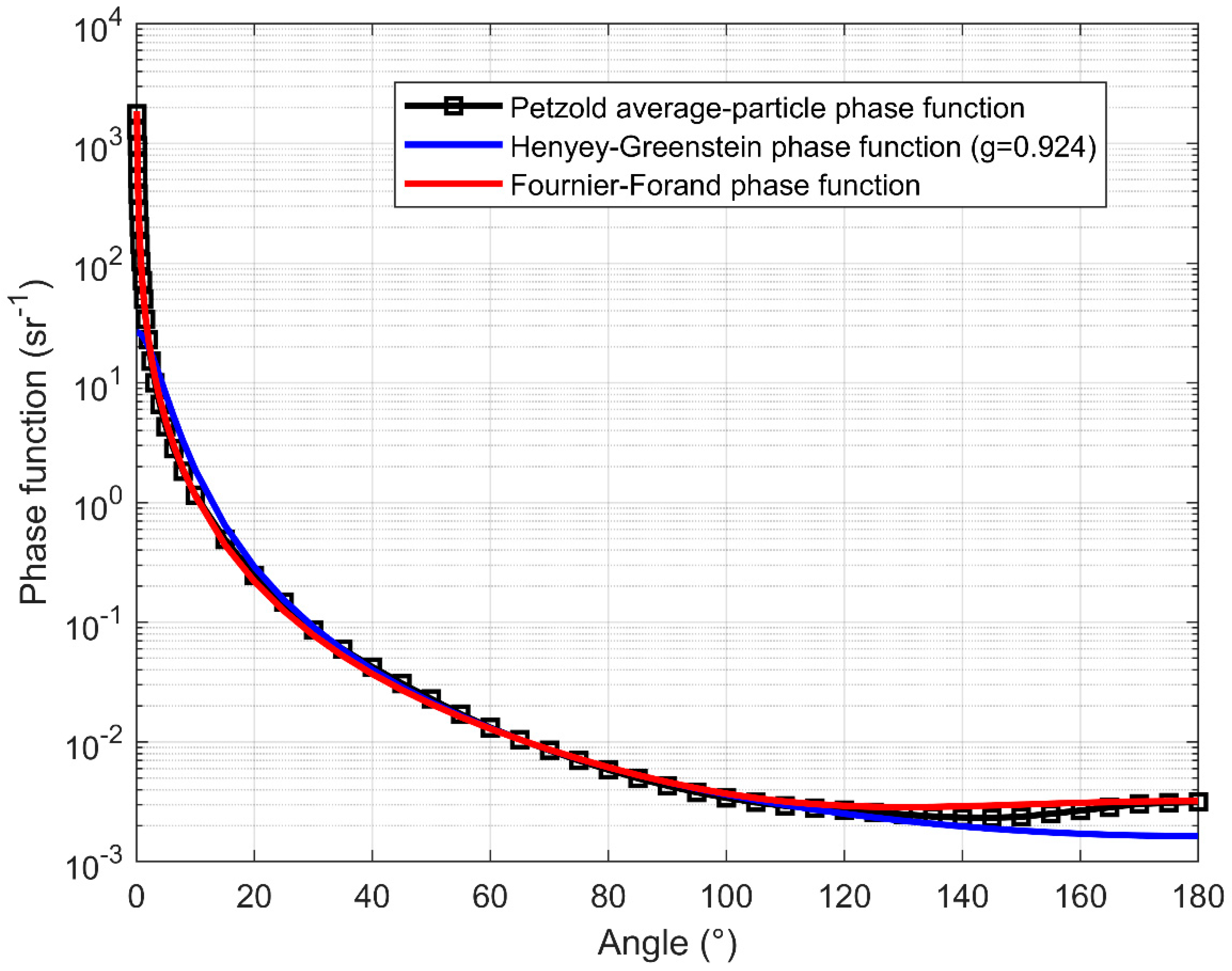
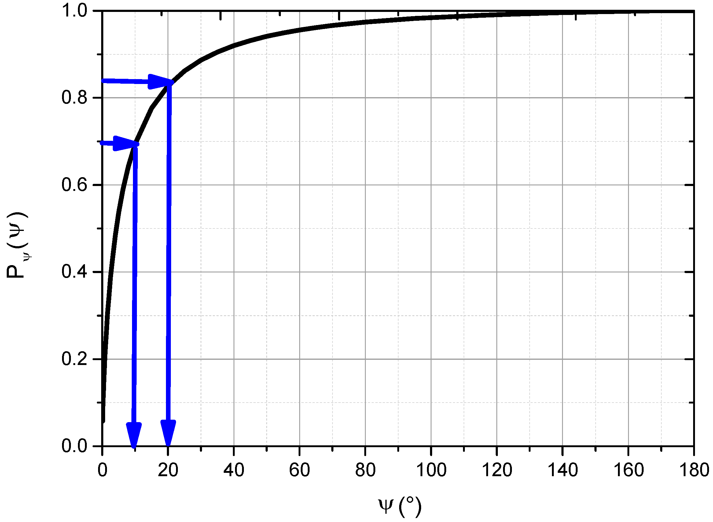
2.2. Determining Scattering Angle: Lookup Table Method

The pdf is fundamental to MC simulation for determining the scattering angle for each photon collision. The spf $\tilde{\beta }(\psi )$ can be interpreted as a pdf in the formula of $\tilde{\beta }(\psi )\sin (\psi )$. The HG spf has been widely used in many MC studies. However, the HG phase function does not work well at small or large scattering angles. As shown in Figure 1, the black curve is the Petzold’s average spf measurement [17], which comprises the most carefully made and widely cited scattering measurements. The red curve shows the Fournier-Forand phase function with the same backscatter fraction as the measured phase function. The blue curve presents the HG phase function; we can see that it does not fit well at small angles (<20°, especially bad for angles of less than 1°) or large angles (>140°). There is a deviation for HG spf among the curves in angles between 140 and 180 degrees because oceanic particles are quite different in their physical properties from interstellar dust, which is initially widely used.

Table 1. The curve-fitting statistics of the two spfs compared with Petzold’s measurements.

SPFs	Angle Limit	Number of Samples	R2	Root Mean Square Error (RMSE)
H-G	all	55	0.3766	323.9334
	[20°,140°]	25	0.9950	0.0115
	<20°	22	0.2662	457.5366
	>140°	8	0.8217	4.2527 × 10−4
FF	all	55	0.9996	14.7719
	[20°,140°]	25	0.9992	0.0088
	<20°	22	0.9996	22.1625
	>140°	8	0.9260	2.1983 × 10−4

shows the curve-fitting statistics of the two spfs compared with Petzold’s measurements. Note that the HG parameter g is 0.924, which already gives the best fit to the Petzold’s measurements, but the curve still does not work well.

$$RMSE=\sqrt{\frac{1}{n}{\displaystyle \sum _{i=1}^n{(y_i-{\widehat{y}}_i)}^2}}$$

(3)

Here, $y_i$ is the difference between spf-calculated and measured data, ${\widehat{y}}_i$ is the mean value of $y_i$, $y_i^{\prime }$ is the relative difference and ${\widehat{y}}_i^{\prime }$ is the mean relative difference.

Though the Fournier-Forand phase function could give the best fit to the Petzold’s measurements of average particle phase function as shown in Figure 1, its cdf (Equation (3)) [18] for $\psi$ would give a complicated formula. Solving the cdf equation of FF for $\psi$ seems impossible. It is numerically more efficient to use Equation (4) to build up a lookup table of $\psi$ vs. $P_{\Psi }(\psi )$ to determine scattering angle.

$$\begin{array}{ll}{P}_{\Psi }^{FF}(\psi )& =\frac{1}{(1-\delta )\delta \upsilon }[(1-{\delta }^{\upsilon +1})-(1-{\delta }^{\upsilon }){\sin }^2(\psi /2)]\\ & +\frac{1}{8}\frac{1-{\delta }_{180}^{\upsilon }}{({\delta }_{180}^{\upsilon }-1){\delta }_{180}^{\upsilon }}\cos \psi {\sin }^2\psi \end{array}$$

(4)

where

$$\upsilon =\frac{3-\mu }{2},\delta =\frac{4}{3{(\mathrm{n}-1)}^2}{\sin }^2(\frac{\psi }{2})$$

(5)

Here, $\mathrm{n}$ is the real part of refraction of the particles, $\mu$ is the slope parameter of the hyperbolic distribution, and ${\delta }_{180}^{\upsilon }$ is $\delta$ at $\psi =180°$.

In this study, we first obtain the cdfs for various spfs using the Kaplan–Meier non-parametric method [19], and then build a LUT with two columns of $\psi$ vs. $P_{\Psi }(\psi )$. The Ψ angle increments in the LUT table are dense and incremental from 0.02° to 5° in a range between 0.1° and 10°; when it reaches 10°, the increments keep constant at 5°. This is mainly because the spfs vary significantly in the small angles, while vary gently in the larger angles. Since the table is discrete, the resulting values are linearly interpolated between the two consecutive values. Petzold’s measurements mentioned above show that linear interpolation is good enough to obtain the results between two discrete values. When a random number $\Re$ is generated, we find the nearest $P_{\Psi }(\psi )$; the corresponding angle $\psi$ is the scattering angle we need. This is illustrated in Figure 2, which shows a Fourier-Forand cdf for $\psi$ vs. $P_{\Psi }(\psi )$ as tabulated using Equation (4). The blue arrows show how drawing a value of $P_{\Psi }(\psi )=0.694$ leads to a scattering angle of $\psi$ about 10 degree, and drawing a value of $P_{\Psi }(\psi )=0.827$ leads to a scattering angle of $\psi$ about 20 degrees.

$$P_{\Psi }(\psi )=\{\begin{array}{c}{P}_{\Psi }({\psi }_{\min }),\mathrm{if}(\Re \le P_{\Psi }({\psi }_{\min }))\\ P_{\Psi }({\psi }_{i+1}),\mathrm{if}(P_{\Psi }({\psi }_i)<\Re <=P_{\Psi }({\psi }_{i+1}))\\ P_{\Psi }({\psi }_{\max }),\mathrm{if}(\Re >P_{\Psi }({\psi }_{\max }))\end{array}$$

(6)

where $P_{\Psi }({\psi }_{\min })$ and $P_{\Psi }({\psi }_{\max })$ are cdf values at the minimum and maximum angles, respectively. $P_{\Psi }({\psi }_i)$ is the cdf of the angle at row $i$.

2.3. Semi-Analytic MC Model

We developed an improved semi-analytic MC simulation model for analytically estimating the probability of photon scatter back to a remote receiver $E(\mathrm{i})$ at collision point i, which is also appropriate for inhomogeneous water:

$$\begin{array}{ll}E(\mathrm{i})& =\frac{\mathrm{p}(\theta )}{4\pi }\Delta \Omega \exp ({\displaystyle \sum _1^i-c(\mathrm{i}){\mathrm{d}}_i})\mathrm{w}(\mathrm{i})\\ & =\frac{\mathrm{p}(\theta )}{4\pi }\frac{A_r}{{(H+z_i)}^2}\exp ({\displaystyle \sum _1^i-c(\mathrm{i}){\mathrm{d}}_i})\mathrm{w}(\mathrm{i})\end{array}$$

(7)

where $\mathrm{p}(\theta )$ is the spf value at angle $\theta$; $\Delta \Omega$ is the small solid angle of collision photon received by a remote detector; $A_r$ means the detector aperture; $H$ is lidar flight height; $z_i$ is the distance from point i to sea surface, which equals the photon’s depth; $c(\mathrm{i})$ is sea water using the beam attenuation coefficient, and ${\mathrm{d}}_i$ is the thickness of each divided layer. Because the solid angle of collision photon received by a remote detector is so small, the cosine value of the actual backscattering line is similar to the line perpendicular to the air/water interface. Therefore, each layer distance ${\mathrm{d}}_i$ is vertical. The analytical lidar geometric model for describing the photon’s scattering event is shown in Figure 3. Before using the equation, we should determine whether the photon’s position is within the receiver field of view (FOV) first.

$$\begin{array}{l}{x_i}^2+{y_i}^2\le A_z\\ A_z={\Omega }_{FOV}{(H+{\mathrm{z}}_i)}^2\end{array}$$

(8)

where ${\Omega }_{FOV}$ is the receiver FOV solid angle; $A_z$ is the area at depth ${\mathrm{z}}_i$ seen by the receiver; $x_i$, $y_i$, and $z_i$ are the photon’s position in Cartesian coordinates.

At each photon scattering event, a photon is scattered into a new trajectory and the scattering angle $\theta$ is determined by the LUT method described in the previous section. Meanwhile, the photon’s weight $\mathrm{w}(\mathrm{i})$ is multiplied by the single scattering albedo $\mathrm{w}(\mathrm{i})$. If a photon’s weight drops under the preset threshold of 10^‒4, a roulette procedure is triggered and employed. In this study, divided layer vertical resolution can reach up to 0.11 m.

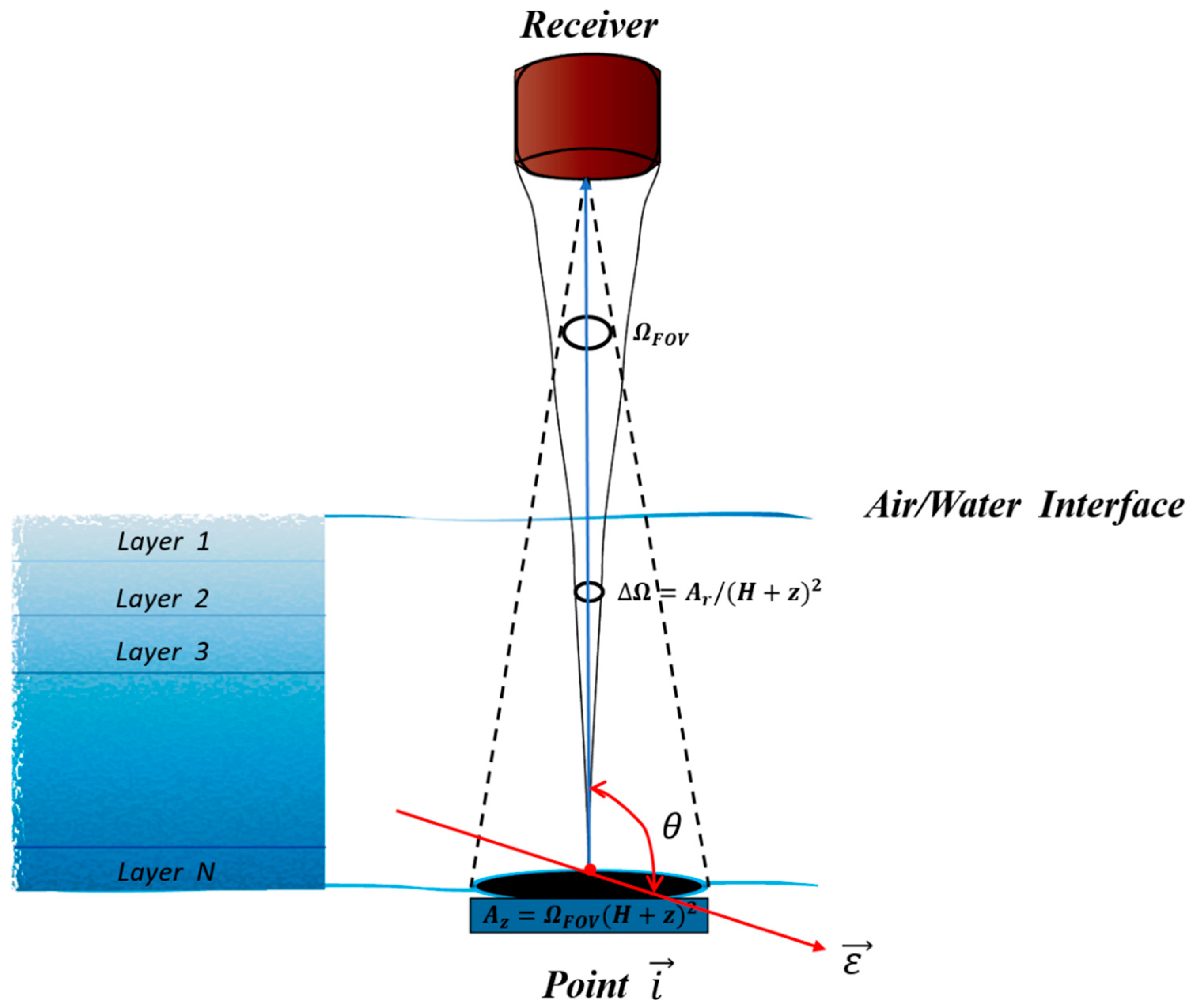
2.4. Boundary Consideration

As a photon reaches the sea surface, an estimation for total transmission $t_t$ of ocean interface due to specific viewing angle and sea wave conditions of rough sea surface [20,21] is given:

$$t_t=t_p\times t_r$$

(9)

where $t_p$ is means the part of transmission under calm sea surface calculated with Snell’s law; and $t_r$ is the part of transmission in a wind-driven roughened surface and can be obtained as a function of wind speed $u$:

$$\{\begin{array}{l}{t}_r=1-1.2\times {10}^{-5}\times u^{3.3},u\le 9\mathrm{m}/\mathrm{s}\\ t_r=1-1.2\times {10}^{-5}\times u^{3.3}\times (0.225u-0.99),u>9\mathrm{m}/\mathrm{s}\end{array}$$

(10)

Actual measurements of bidirectional reflectance distribution functions (BRDFs) of ocean bottom materials like sand or sea grass canopies have rarely been made. Because of the lack of measurements and models of the BRDF for actual ocean bottom materials, it is usually assumed that a bottom is a Lambertian reflecting surface [22]. In this study, the sea bottom is simply treated as a Lambertian surface, and for that reason lidar bathymetry simulation is not useful for our purposes. Its reflectivity is the same in all directions. A reflection event is forced by multiplying the photon’s weight by sea bottom albedo.

3. Simulation Results

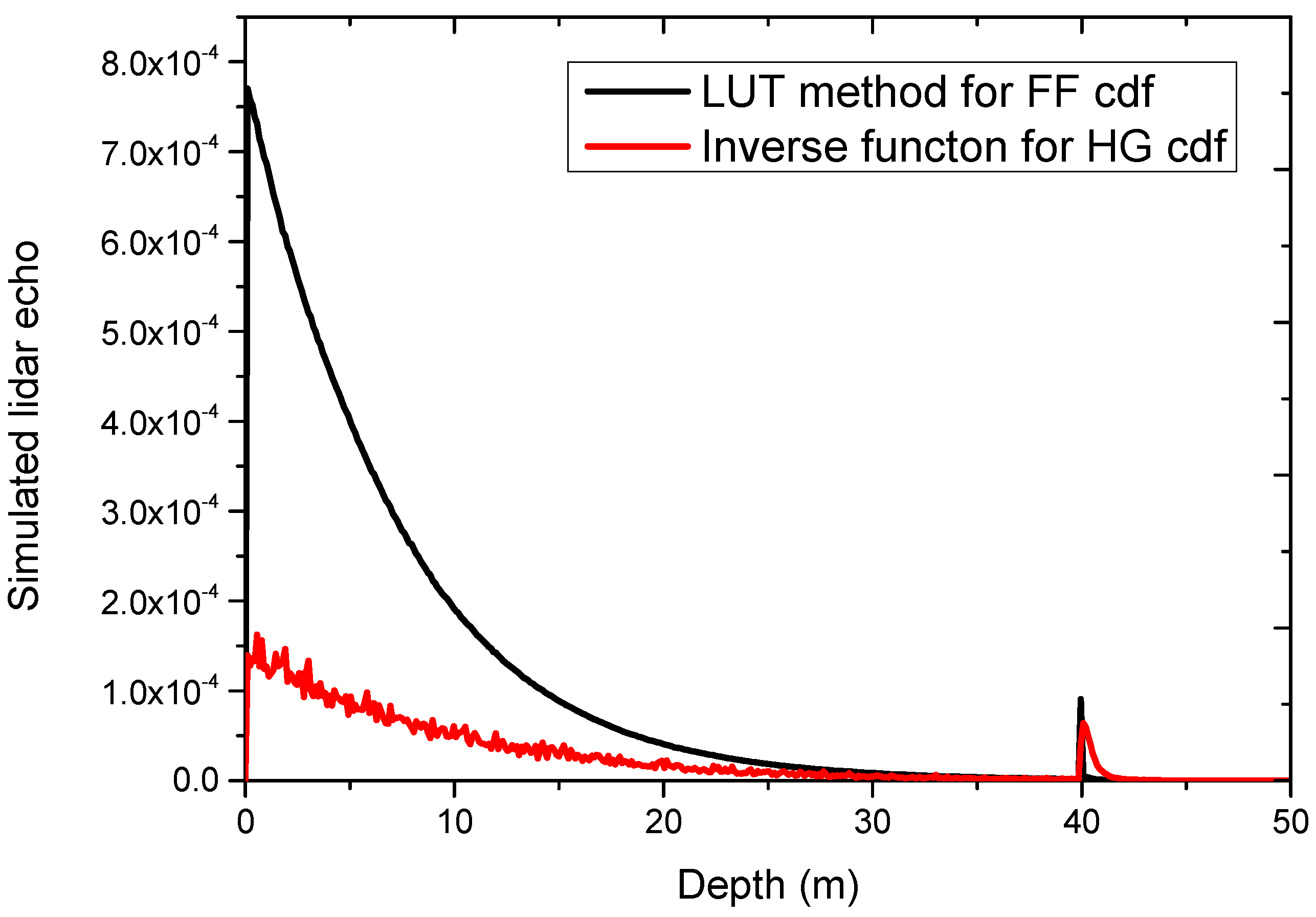
3.1. Simulation Comparison between Inverse Function for HG cdf and LUT Method for FF cdf

The inverse equation of HG cdf for scatter angle $\psi$ is

$$\psi ={\cos }^{-1}[\frac{1+g^2}{2g}-\frac{1}{2g}{(\frac{1-g^2}{1+g-2g\Re })}^2]$$

(11)

Figure 4 shows the simulation comparison between the inverse cdf method for HG and the LUT method for FF. Simulations were conducted using a total of 10,000,000 photons for a given detector height of $H=300\mathrm{m}$, $FOV=50\mathrm{mrad}$, detector aperture of $A=0.06{\mathrm{m}}^2$, sea bottom depth of $d=40\mathrm{m}$, vertical layer resolution of 0.11 m, water absorption coefficient of $\alpha =0.04{\mathrm{m}}^{-1}$, scattering coefficient of $b=0.06{\mathrm{m}}^{-1}$, and sea bottom albedo of ${\rho }_b=0.03$. The given $n$ and $\mu$ for FF spf were 1.10 and 3.62, respectively. The HG parameter was set to 0.924. It took 129 s and 140 s for the LUT method and ICDF method simulations, respectively. It shows that the simulation curve using the LUT method of FF is larger and more stable than using the ICDF method of HG under the same input condition. It may be because the forward scattering of HG spf is much less than that of the Petzold’s measurements (see Figure 1). Besides, the back scattering is also less; therefore, the $\mathrm{p}(\theta )$ value in Equation (2) is less. We can see that the black curve by LUT method looks smoother than the red curve by the inverse function method. The adjusted R-square (N = 498) between the two curves in Figure 1 is 0.948. The residual sum of squares is 3.2 × 10⁻⁸. The RMSE is 8.03 × 10⁻⁶. The min value, max value, mean value, and standard deviation of the red curve are 1.54 × 0⁻⁸, 7.70 × 0⁻⁴, 9.82 × 0⁻⁵, and 1.73 × 0⁻⁴, respectively. The min value, max value, mean value, and standard deviation of the black curve are 1.11 × 10⁻⁹, 1.63 × 10⁻⁴, 2.48 × 10⁻⁵, and 3.53 × 10⁻⁵, respectively (see

Table 2. The statistics of the curves in Figure 1 by the two methods.

Methods	Number of Samples	Min.	Max.	Mean	Standard Deviation (SD)	R2 between the Two Curves	RMSE between the Two Curves
ICDF	498	1.11 × 10−9	1.63 × 10−4	2.48 × 10−5	3.53 × 10−5	0.948	8.03 × 10−6
LUT	498	1.54 × 10−8	7.70 × 10−4	9.82 × 10−5	1.73 × 10−4

). The signal intensity by LUT method appears higher than ICDF method: This is because the ICDF method to calculate the backscattering probability return to receiver was to obtain a possible certain backscattering angle, which may be less than the small receive angle range, while the LUT method to calculate the backscattering probability return to receiver was to obtain the integrals between two discrete values, which is a little larger than the small receive angle range. The standard deviation of the red curve by ICDF method is more than 5 times larger than the black curve by LUT method. It looks like there is more noise and disturbance in the red curve by ICDF method under the same preset parameters. The results also indicate the LUT method is more stable than the inverse function method. We also find that the sea bottom curve based on the LUT method for FF cdf has less pulse widening effect than the inverse function method for HG cdf.

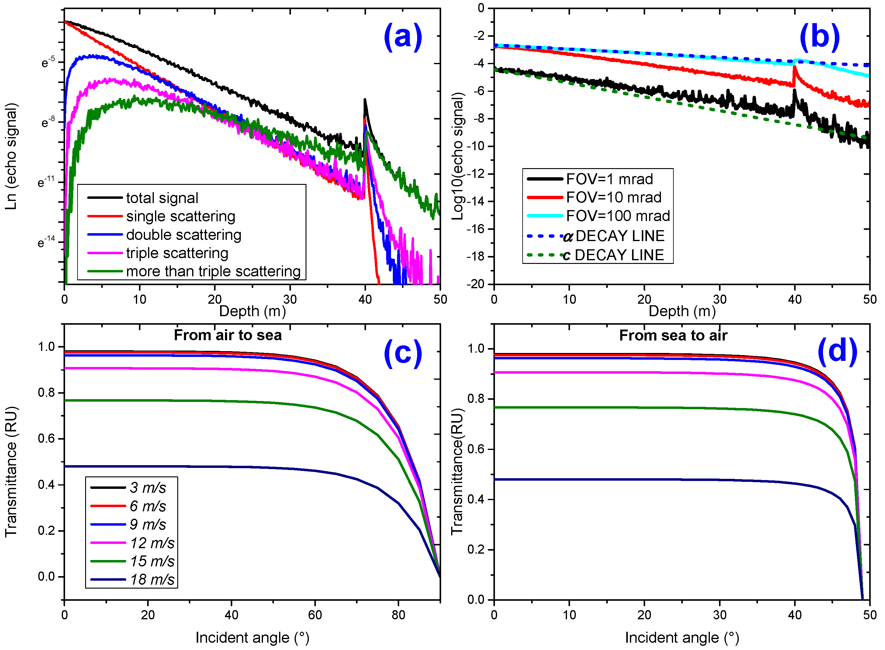
3.2. Multiple Scattering and Wind-Driven Roughened Sea Surface Effect

Influences of multiple scattering and wind-driven roughened sea surface conditions on simulation results were then analyzed. We separated the first order of scattering, second order of scattering, third order of scattering, and more than third order of scattering parts in the total scattering signal, as shown in Figure 5a. The black line is the total signal, which is the sum of the single, double, triple and more than triple scattering event curves. Figure 5a shows that the single scattering signal decreases as depth increases, while multiple scattering signal increases first and then decreases. This is because, as the photon travels forward, multiple scattering occurs more frequently in water. Besides, the signal is the deepest depth the photon attained prior to scattering back to the surface and being detected. It also shows that the single, double, triple and greater than triple scattering events curves cross at about 20 m. The multiple scattering occurs more frequently as the water scattering coefficient becomes larger. When the water scattering coefficient is large, the depth of curves cross decreases, and the depth increases when the water scattering coefficient is small. The first order of scattering in logarithmic form decreases linearly with the increase of depth, which agrees with Mobley’s conclusion that light falls exponentially in water [1], and it indicates that our simulation method is correct and feasible. The contribution of high-order scattering signal increases with depth, until it dominates at a certain depth. Figure 5b shows the slope of return signal, namely, lidar effective attenuation coefficient (K_sys) falls between beam attenuation coefficient $c$ and absorption coefficient $\alpha$. The system attenuation coefficient, K_sys, lies somewhere between $\alpha$ and $c$, and is dependent on the relative values of the transmitter beam spot size, transmitter divergence, receiver aperture, and receiver field of view. As Figure 5b shows, we can see that the cyan curve using a narrow FOV fits well with the blue curve of $c$ and the black curve using a large FOV fits well with the dark green curve of $\alpha$. It approaches $c$ with a narrow FOV and approaches $\alpha$ with a large FOV. K_sys approaches with a narrow field of view c since almost all of the light that had been scattered was not detected by the receiver; thus, the decay rate of the backscatter signal is the sum of $\alpha$ and b. Since the field of view was large enough, K_sys approaches α since the only light lost at the receiver was what had been absorbed. However, for a very large beam and large receiver aperture and field of view, K_sys approaches $\alpha +b_b$ since almost all of the forward propagating photons remain in the receiver FOV until absorbed or scattered in the backward direction. However, when the field of view was large enough, K_sys approaches α, since the only light lost at the receiver was what had been absorbed. These results agree with previous studies [23,24,25]. They indicate that the configuration of multiple FOV applied for lidar system is useful for optical properties’ inversion in various types of water. Figure 5c,d show the influence of wind-driven roughened sea surface on simulation signals. The incident angle in Figure 5c,d is the lidar incident angle. The reason why it spans to about 90 degrees in the “From air to sea” plot, but only to about 48 degrees in the “From sea to air” plot, is due to the critical angle for total internal reflection. We can see that the lidar transmittance coefficients remain unchanged when wind speed is less than 9 m/s, but it decreases significantly when the wind speed is greater than 9 m/s. It indicates that both wind-driven roughened sea surface and multiple scattering have significant effects on simulation results, which should not be ignored.

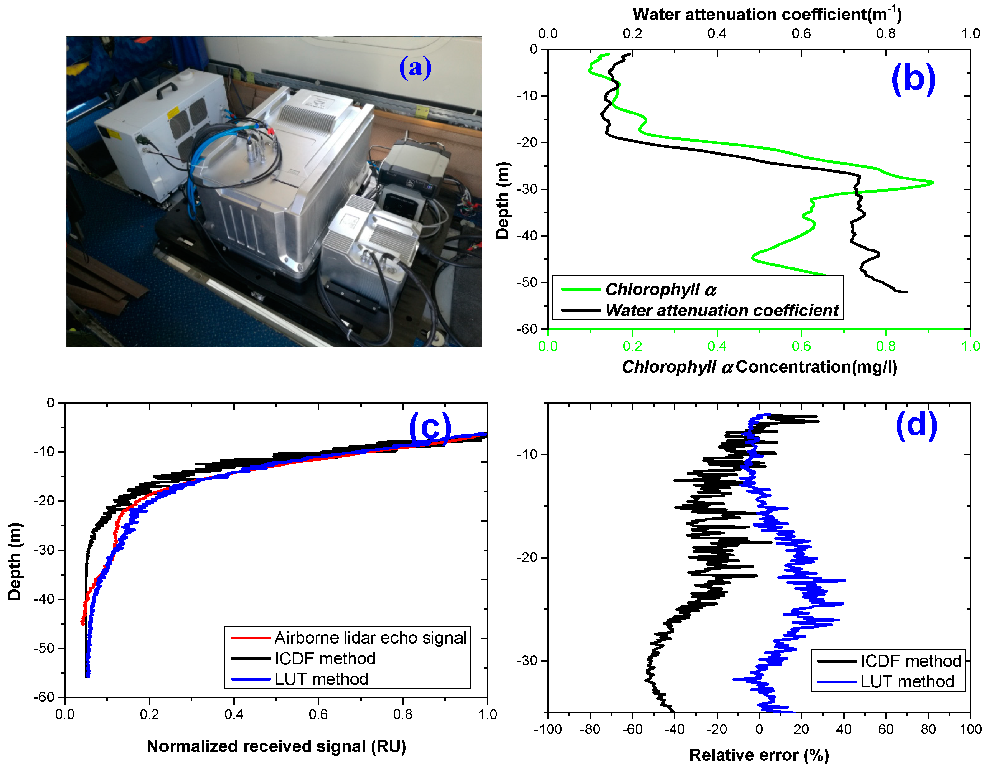
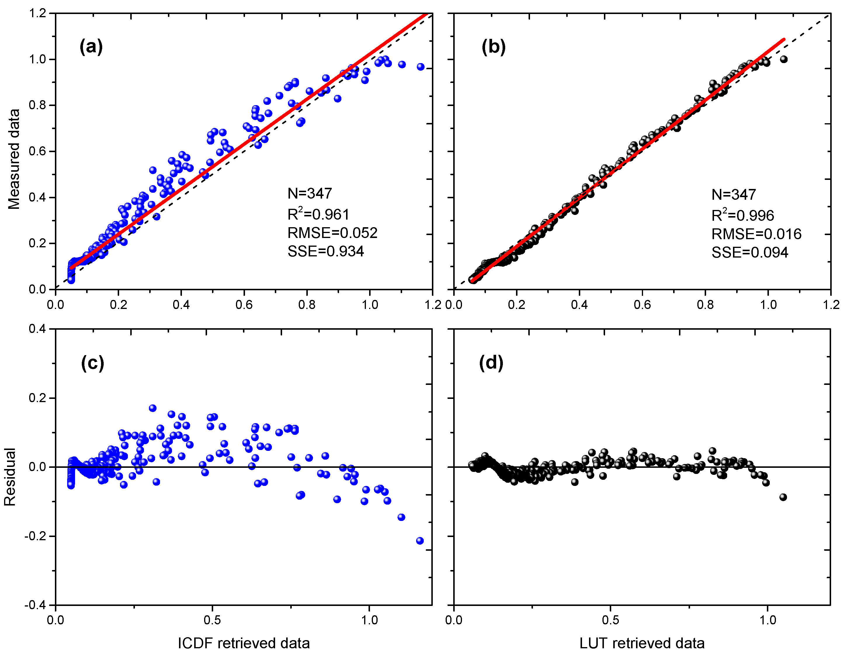
3.3. Simulated-Signal vs. Airborne Lidar Measured-Signal

Subsequently, simulation results (from both LUT and ICDF methods) were compared with airborne lidar measurements. The experimental airborne oceanic lidar was developed by the Shanghai Institute of Optics and Fine Mechanics (SIOM), Chinese Academy of Sciences (Figure 6a). The transmitting system utilized a 532 nm frequency-doubled Nd:YAG laser. Its pulse duration is 1.5 ns, and pulse repetition rate (PRF) is 1 kHz. The detector telescope’s diameter is 200 mm and FOV is 40 mrad. The layer thickness employed in our simulation is 0.11 m; the phase function lookup table was kept unchanged during a simulation process. The profile optical properties of sea water measured at the station (109°43.808′ E, 18°2.205′ N) in Sanya Bay in the South China Sea on 12 March 2018 were input into the model, as shown in Figure 6b. The green line is the chlorophyll a concentration profile, and the black line represents water attenuation coefficient profile. We can see that a subsurface chlorophyll maximum (SCM) layer exists at about 30 m. Clearly, most current MC simulation methods based on the assumption of optically vertical homogeneous are no longer suitable. Figure 6c shows the comparison between simulation signal based on our method with airborne lidar measured-signal. The simulations were conducted using a total of 10,000,000 photons and actual lidar detector height is H = 307 m. We find that the simulated curve using the LUT method (blue line) agrees well with the lidar measured-signal (red line). The ICDF method appears to overestimate the actual signal, which is because the ICDF method used to calculate the backscattering probability return to receiver obtained a possible certain backscattering angle, which is less than small receive angle range. The LUT method appears to underestimate the actual signal at greater depths and also at shallower depths, crossing at about 20 m. This is because the LUT method used to calculate the backscattering probability return to receiver obtained the integrals between two discrete values, which is a little larger than small receive angle range at deeper depths. It may be better to set the LUT increments according to the solid receiver angle. Figure 6d shows the relative errors between simulation and measurements for the LUT method within 14% mean relative error and for the ICDF method within 22% mean relative error. We can see that the relative error was less than 10% for the LUT method and less than 20% for the ICDF method within 20 m. Both methods have the maximum relative errors when the depth is between 25 and 30 m, where there was a chlorophyll maximum scattering layer. It may be due to the fact that the spfs in our study are no longer applicable when reaching the chlorophyll maximum scattering layer. Figure 7 shows the regression plots of simulated-signal vs. airborne lidar measured-signal. Figure 7a,b presents the regression plots of ICDF and LUT retrieved data vs. measured data, respectively. Figure 7c,d presents the residual plots of ICDF and LUT, respectively. It shows that the adjusted R-square between simulation and measurements (N = 347) for LUT method (R² = 0.996) is larger than that by ICDF method (R² = 0.996). The data retrieved from both methods have significant correlations with measured data, although the RMSE by LUT method (RMSE = 0.016) is relatively smaller than that by ICDF method (RMSE = 0.052). As Figure 7c,d shows, the LUT method has relatively smaller residual than that by ICDF method in almost all data. In general, the results indicate that the LUT method is effective for solving complicated or even unsolvable inverse cumulative distribution function of various scattering phase functions, and it significantly improves modeling accuracy.

4. Conclusions

In this study, we introduced an improved semi-analytic MC radiative transfer model based on the LUT method and a lidar geometric model for scattering event, which is also applicable to inhomogeneous water. Comparison of simulation and measurements indicates that our method is effective for solving complicated or even unsolvable inverse cumulative distribution function of various scattering phase functions and for significantly improving modeling accuracy. This model also considers multiple scattering, wind-driven roughened sea surface and water optical inhomogeneous effects. Thus, fundamental radiative transfer problems in oceanographic lidar and effects of a host of environmental factors on lidar system performance can be addressed. We plan to apply our method to in-situ measured spfs, especially subsurface phytoplankton scattering spfs. In addition, simulation results will be used to study the relationships between lidar effective coefficients and water bio-optical properties for quantificational applications. More comparisons between measurements and simulations will be carried out to improve our method.

References

1. Mobley, C.D. Light and Water: Radiative Transfer in Natural Waters; Academic Press: Cambridge, MA, USA, 1994. [Google Scholar]
2. Zhai, P.W.; Kattawar, G.W.; Yang, P. Impulse response solution to the three-dimensional vector radiative transfer equation in atmosphere-ocean systems. I. Monte Carlo method. Appl. Opt. 2008, 47, 1037–1047. [Google Scholar] [CrossRef] [PubMed]
3. Zhai, P.-W.; Kattawar, G.W.; Yang, P. Impulse response solution to the three-dimensional vector radiative transfer equation in atmosphere-ocean systems. II. The hybrid matrix operator--Monte Carlo method. Appl. Opt. 2008, 47, 1063–1071. [Google Scholar] [CrossRef] [PubMed]
4. Ramella-Roman, J.C.; Prahl, S.A.; Jacques, S.L. Three Monte Carlo programs of polarized light transport into scattering media: Part I. Opt. Express 2005, 13, 4420–4438. [Google Scholar] [CrossRef] [PubMed]
5. Ramella-Roman, J.C.; Prahl, S.A.; Jacques, S.L. Three Monte Carlo programs of polarized light transport into scattering media: Part II. Opt. Express 2005, 13, 10392–10405. [Google Scholar] [CrossRef] [PubMed]
6. Berrocal, E.; Sedarsky, D.L.; Paciaroni, M.E.; Meglinski, I.V.; Linne, M.A. Laser light scattering in turbid media Part I: Experimental and simulated results for the spatial intensity distribution. Opt. Express 2007, 15, 10649–10665. [Google Scholar] [CrossRef] [PubMed]
7. Gordon, H.R. Interpretation of airborne oceanic lidar: Effects of multiple scattering. Appl. Opt. 1982, 21, 2996–3001. [Google Scholar] [CrossRef] [PubMed]
8. Poole, L.R.; Venable, D.D.; Campbell, J.W. Semianalytic Monte Carlo radiative transfer model for oceanographic lidar systems. Appl. Opt. 1981, 20, 3653–3656. [Google Scholar] [CrossRef] [PubMed]
9. Chen, P.; Pan, D.; Mao, Z.; Liu, H. Semi-analytic Monte Carlo radiative transfer model of laser propagation in inhomogeneous sea water within subsurface plankton layer. Opt. Laser Technol. 2019, 111, 1–5. [Google Scholar] [CrossRef]
10. Otsuki, S. Multiple scattering of polarized light in turbid infinite planes: Monte Carlo simulations. J. Opt. Soc. Am. A 2016, 33, 988–996. [Google Scholar] [CrossRef] [PubMed]
11. Berrocal, E.; Meglinski, I.; Jermy, M. New model for light propagation in highly inhomogeneous polydisperse turbid media with applications in spray diagnostics. Opt. Express 2005, 13, 9181–9195. [Google Scholar] [CrossRef] [PubMed]
12. Xu, M. Electric field Monte Carlo simulation of polarized light propagation in turbid media. Opt. Express 2004, 12, 6530–6539. [Google Scholar] [CrossRef] [PubMed]
13. Seteikin, A.Y. Monte Carlo analysis of laser radiation propagation in multilayer biological materials. Opt. Spectrosc. 2005, 99, 659–662. [Google Scholar] [CrossRef]
14. Henyey, L.C.; Greenstein, J.L. Diffuse radiation in the galaxy. Astrophys. J. 1941, 93, 70–83. [Google Scholar] [CrossRef]
15. Fournier, G.R.; Forand, J.L. Analytic phase function for ocean water. Proc. SPIE Int. Soc. Opt. Eng. 1994, 2258, 194–201. [Google Scholar]
16. Jacques, S.L. Monte Carlo modeling of light transport in tissue (steady state and time of flight). In Optical-Thermal Response of Laser-Irradiated Tissue; Springer: Berlin, Germany, 2010; pp. 109–144. [Google Scholar]
17. Petzold, T.J. Volume Scattering Functions for Selected Ocean Waters; Scripps Institution of Oceanography: La Jolla, CA, USA, 1972. [Google Scholar]
18. Fournier, G.R. Computer-based underwater imaging analysis. Proc. SPIE Int. Soc. Opt. Eng. 1999, 3761, 62–70. [Google Scholar]
19. Lawless, J.F. Statistical Models and Methods for Lifetime Data, 2nd ed.; John Wiley & Sons, Inc.: Hoboken, NJ, USA, 2011. [Google Scholar]
20. Estes, L.E.; Fain, G.; Harris, J.D. Laser beam propagation through the ocean’s surface. In Proceedings of the OCEANS 96 MTS/IEEE Conference Proceedings, The Coastal Ocean—Prospects for the 21st Century, Fort Lauderdale, FL, USA, 23–26 September 1996; Volume 8, pp. 87–94. [Google Scholar]
21. Li, T.; Ao, F.-L.; Ou, Y. The study of blue and green laser through seawater interface. In Proceedings of the 15th Annual Conference of Information Theory and the First National Network Coding Academic Conference Proceedings of the China Electronics Society, Qing Dao, ShanDong, China, 15–20 Augest 2008; pp. 297–301. [Google Scholar]
22. Mobley, C.D.; Zhang, H.; Voss, K.J. Effects of Optically Shallow Bottoms on Upwelling Radiances: Bidirectional Reflectance Distribution Function Effects. Limnol. Oceanogr. 2003, 48, 337–345. [Google Scholar] [CrossRef]
23. Feygels, V.I.; Wright, C.W.; Kopilevich, Y.I.; Surkov, A.I. Narrow-field-of-view bathymetrical lidar: Theory and field test. In Proceedings of the SPIE’s 48th Annual Meeting on Optical Science and Technology, San Diego, CA, USA, 3–8 August 2003; pp. 1–11. [Google Scholar]
24. Allocca, A.D.M.; London, M.A.; Curran, T.P.; Concannon, B.M.; Contarino, V.M.; Prentice, J.; Mullen, L.J.; Kane, T.J. Ocean water clarity measurement using shipboard lidar systems. Proc. SPIE 2002, 4488, 106–114. [Google Scholar]
25. Concannon, B.M.; Prentice, J.E. LOCO with a Shipboard Lidar; Naval Air Systems Command: Patuxent River, MD, USA, 2008. [Google Scholar]
Figure 1. Log-linear plot of various scattering phase functions. The black curve is the standard phase function measured by Petzold. The red curve shows the Fournier-Forand phase function with the same backscatter fraction as the measured phase function. The blue curve presents the Henyey-Greenstein phase function.
Applsci 09 00048 g001
Figure 2. A cdf of Fournier-Forand phase function as tabulated using Equation (4).
Applsci 09 00048 g002
Figure 3. Lidar geometric model for analytically estimating the probability of photon scatter back to a remote receiver.
Applsci 09 00048 g003
Figure 4. Simulation comparison between inverse equation for Henyey-Greenstein (HG) cumulative distribution function (cdf) and lookup table (LUT) method for Fournier-Forand (FF) cdf. The black curve is based on the LUT method for FF cdf, and the red curve is based on the inverse function for HG cdf.
Applsci 09 00048 g004
Figure 5. Wind-driven roughened sea surface and multiple scattering have significant effects on simulation results in logarithmic form: (a) Separation of contributions by different scattering order in the total signal, (b) field of view (FOV) influence on return signal, (c) influence of wind-driven roughened sea surface various incident angles on transmittance from air to sea, and (d) influence of wind-driven roughened sea surface various incident angles on transmittance from sea to air.
Applsci 09 00048 g005
Figure 6. Simulated-signal vs. airborne lidar measured-signal: (a) Airborne lidar photo, (b) chlorophyll and c ( z ) profiles, (c) simulated signal vs. lidar measured-signal, and (d) error curve of comparison.
Applsci 09 00048 g006
Figure 7. Regression plots of simulated-signal vs. airborne lidar measured-signal. (a) Regression plot of inverse cdf (ICDF) retrieved data vs. measured data, (b) regression plot of LUT retrieved data vs. measured data, (c) residual plot of ICDF retrieved data vs. measured data, (d) residual plot of LUT retrieved data vs. measured data.
Applsci 09 00048 g007