Free Transverse Vibration of Rectangular Orthotropic Plates with Two Opposite Edges Rotationally Restrained and Remaining Others Free

Abstract

Many types of engineering structures can be effectively modelled as orthotropic plates with opposite free edges such as bridge decks. The other two edges, however, are usually treated as simply supported or fully clamped in current design practice, although the practical boundary conditions are intermediate between these two limiting cases. Frequent applications of orthotropic plates in structures have generated the need for a better understanding of the dynamic behaviour of orthotropic plates with non-classical boundary conditions. In the present study, the transverse vibration of rectangular orthotropic plates with two opposite edges rotationally restrained with the remaining others free was studied by applying the method of finite integral transforms. A new alternative formulation was developed for vibration analysis, which provides much easier solutions. Exact series solutions were derived, and the excellent accuracy and efficiency of the method are demonstrated through considerable numerical studies and comparisons with existing results. Some new results have been presented. In addition, the effect of different degrees of rotational restraints on the mode shapes was also demonstrated. The present analytical method is straightforward and systematic, and the derived characteristic equation for eigenvalues can be easily adapted for broad applications.

1. Introduction

In Civil Engineering, many types of bridge decks and floor systems can be effectively modeled as orthotropic plates with opposite free edges. In practice, the other two edges of these structures are mostly not classical (i.e., neither simply supported nor fully clamped). In order to consider actual boundary conditions, these edges are intermediate between simply-supported and fully-clamped, which can be modelled as elastically restrained against rotation (i.e., rotationally restrained). However, vibration analysis of plate structures with non-classical boundary conditions involves complicated mathematical procedures. Therefore, in the design practice, the analyses of bridge decks and floors are often simplified based on a beam idealization. This simplification is not always suitable for short-span plate structures. Motivated by the extensive applications of structurally orthotropic plates in engineering structures, the present investigation deals with free transverse vibration of the rectangular orthotropic plates with two opposite edges rotationally restrained and leaving the remaining others free (i.e., R–F–R–F).

A considerable amount of literature has been published on analytical solutions for vibration of orthotropic plates with classical boundary conditions such as simply supported, clamped, and free [1,2,3,4]. In parallel, vibration of rectangular plates with elastically restrained edges has attracted considerable attention since the 1950s [5,6,7,8,9,10,11]. These studies focused primarily on the approximate estimation of natural frequencies by using Rayleigh method and Ritz method. Furthermore, most studies were devoted to isotropic plates with elastically restrained and simply supported edges. Limited research has been conducted to study orthotropic plates with elastically restrained and free edges. Laura and his colleagues [12,13] investigated orthotropic plates with three edges elastically restrained and the fourth edge free (i.e., R–R–R–F) and two adjacent edges elastically restrained and the other adjacent edges free (i.e., R–R–F–F) by Rayleigh method. Similarly, orthotropic plates with the edges elastically restrained against rotation and a free, straight corner cut-out was studied in [14]. The results reported in these three works are limited to the fundamental frequency. Grace and Kennedy [15] studied the dynamic response of orthotropic plate having clamped-simply supported and free-free boundary conditions (i.e., C–F–S–F). Liu and Huang [16] directly extended the semi-analytical finite difference method reported in [8] to free vibrations of orthotropic plates with elastically restrained and free edges. Some eigenvalues for R–F–R–F orthotropic plates have been reported. On top of that, to the best knowledge of the authors, no exact analytical solution is currently available for transverse vibration of R–F–R–F orthotropic plates.

Although approximate solutions and numerical modelling may be sufficient for practical purposes, exact solutions are desirable to assess the effectiveness of these approximate solutions. Recently, an analytical method of finite integral transforms has been extensively applied to obtained the exact series solutions of bending of plates [17,18,19,20]. By using this method, the authors [21,22] obtained the exact solutions for bending of R–R–R–R and R–F–R–F orthotropic plates with integral kernel of $sin{\alpha }_{m}xsin{\beta }_{n}y$ and $sin{\alpha }_{m}xcos{\beta }_{n}y$, respectively. However, it has been found that the formulation of the finite integral transform method used for the bending problems of orthotropic plates cannot be directly applied to vibration problems [23], which involve solving a highly non-linear equation and would be quite difficult.

In the present study, an alternative formulation of the finite integral transform method was developed for the free vibration of R–F–R–F rectangular orthotropic plates. Through a systematic solving procedure, the characteristic equation for eigenvalues can be derived. The frequency parameters and corresponding mode shapes can be obtained by solving the eigenvalue problem numerically. A convergence study and extensive comparisons with previous results were conducted to verify the accuracy and efficiency of the present method. The mode shapes of an orthotropic plate having different degrees of rotational restraints along the opposite edges were also illustrated.

2. Formulation and Methodology

As illustrated in Figure 1, a rectangular orthotropic thin plate is considered herein, which has two opposite edges free (i.e., $y=0$ and $y=b$) and the others rotationally restrained (i.e., $x=0$ and $x=a$). The differential equation for the free transverse vibration of orthotropic plates is [1]

$$D_x\frac{{\partial }^{4}w}{\partial x^4}+2H\frac{{\partial }^{4}w}{\partial x^2\partial y^2}+D_y\frac{{\partial }^{4}w}{\partial y^4}+\rho h\frac{{\partial }^{2}w}{\partial t^2}=0$$

(1)

in which $w(x,y,t)$ is the displacement function; $\rho$ is the density of the plate; $D_x$ and $D_y$ are the flexural rigidity in the x-direction and y-direction, respectively; and H is effective torsional rigidity.

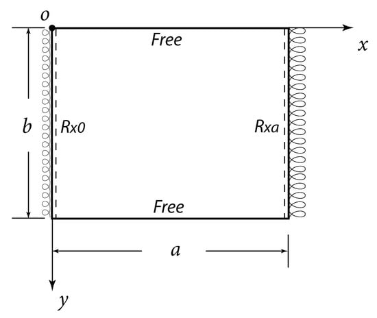
Figure 1. Orthotropic plate with opposite rotationally restrained and free edges (R–F–R–F).

The frequency of sinusoidal oscillations is denoted by $\omega$. Then, the displacement function of the plate $w(x,y,t)$ can be given by

$$w(x,y,t)=W(x,y)e^{i\omega t}$$

(2)

Substituting Equation (2) into Equation (1), it can be obtained

$$D_x\frac{{\partial }^{4}W}{\partial x^4}+2H\frac{{\partial }^{4}W}{\partial x^2\partial y^2}+D_y\frac{{\partial }^{4}W}{\partial y^4}-{\omega }^2\rho hW=0$$

(3)

For simplicity, the partial differentiation was denoted by a comma (e.g., $\frac{dw}{dx}=w{,}_x$). The boundary conditions of the plate can be written as

$$\begin{array}{c}w=0,M_x=-D_x\left(w{,}_{xx}+{\nu }_{y}w{,}_{yy}\right)=-R_{x0}w{,}_{x}atx=0\hfill \end{array}$$

(4a)

$$\begin{array}{c}w=0,M_x=-D_x\left(w{,}_{xx}+{\nu }_{y}w{,}_{yy}\right)=R_{xa}w{,}_{x}atx=a\hfill \end{array}$$

(4b)

$$\begin{array}{c}{M}_y=-D_y\left(w{,}_{yy}+{\nu }_{x}w{,}_{xx}\right)=0aty=0,b\hfill \end{array}$$

(4c)

$$\begin{array}{c}{V}_y=-D_{y}w{,}_{yyy}-\left(H+2D_{xy}\right)w{,}_{yxx}=0aty=0,b\hfill \end{array}$$

(4d)

where $M_x$ and $M_y$ are the bending moments, $V_y$ is the effective shear force, and $R_{x0}$ and $R_{xa}$ are rotational stiffness as shown in Figure 1. In order to describe the rotational stiffness regarding the flexural stiffness of the plate, a rotational fixity factor r was developed by Zhang and Xu [21] as

$$\begin{array}{cc}\hfill r_{x0}& =\frac{1}{{\displaystyle 1+3\frac{D_x}{R_{x0}a}}}\hfill \end{array}$$

(5a)

$$\begin{array}{cc}\hfill r_{xa}& =\frac{1}{{\displaystyle 1+3\frac{D_x}{R_{xa}a}}}\hfill \end{array}$$

(5b)

Rotational fixity factors have a range from 0 to 1. Then, a general boundary condition can be modelled by different values. For instance, the limiting cases, simply supported and fully clamped boundary conditions, will be treated as $r=0$ and $r=1$, respectively. Thus, it can be obtained from Equations (5) that

$$\begin{array}{c}\hfill R_{x0}a=\frac{3r_{x0}}{1-r_{x0}}{D}_x\end{array}$$

(6a)

$$\begin{array}{c}\hfill R_{xa}a=\frac{3r_{xa}}{1-r_{xa}}{D}_x\end{array}$$

(6b)

At first, the boundary conditions were rearranged by separately taking the finite cosine transform (FCT) of Equations (4a) and (4b) with respect to y and the finite sine transform (FST) of Equations (4c) and (4d) with respect to x. As a result, the boundary conditions can be expressed as

$$\begin{array}{cc}\hfill D_x\widehat{W}{,}_{xx}(0,n)& =R_{x0}\widehat{W}{,}_x(0,n)\hfill \end{array}$$

(7a)

$$\begin{array}{cc}\hfill D_x\widehat{W}{,}_{xx}(a,n)& =-R_{xa}\widehat{W}{,}_x(a,n)\hfill \end{array}$$

(7b)

$$\begin{array}{cc}\hfill \overline{W}{,}_{yy}(m,y)& ={\nu }_x{\alpha }_m^2\overline{W}(m,y),fory=0,b\hfill \end{array}$$

(7c)

$$\begin{array}{cc}\hfill \overline{W}{,}_{yyy}(m,y)& =\frac{H+2D_{xy}}{D_y}{\alpha }_m^2\overline{W}{,}_y(m,y),fory=0,b\hfill \end{array}$$

(7d)

Subsequently, the governing equation of Equation (3) is solved by using the method of finite integral transform. In this paper, the joint finite integral transform is defined by applying FST with respect to x with m as the subsidiary variable and the FCT in regard to y with n.

$$\widehat{\overline{W}}(m,n)={\int }_0^a{\int }_0^{b}W(x,y)sin{\alpha }_{m}xcos{\beta }_{n}ydxdy$$

(8)

where

$${\alpha }_m=\frac{m\pi }{a},{\beta }_n=\frac{n\pi }{b}(m=1,2,3,\dots ,n=0,1,2,3,\dots )$$

(9)

The transform inversion of Equation (8) can be obtained as [24]

$$W(x,y)=\frac{4}{ab}\sum _{m=1}^{\infty }\sum _{n=0}^{\infty }{\epsilon }_n\widehat{\overline{W}}(m,n)sin{\alpha }_{m}xcos{\beta }_{n}y$$

(10)

where

$${\epsilon }_n=\left\{\begin{array}{cc}1/2,& n=0\\ 1,& n\ne 0\end{array}\right.$$

(11)

Taking joint finite sine and cosine transforms on both sides of Equation (3), it gives

$${\int }_0^a{\int }_0^b{\nabla }_o^{4}W(x,y)sin{\alpha }_{m}xcos{\beta }_{n}ydxdy-{\omega }^2\rho h\widehat{\overline{W}}(m,n)=0$$

(12)

where

$${\nabla }_o^4=D_x\frac{{\partial }^4}{\partial x^4}+2H\frac{{\partial }^4}{\partial x^2\partial y^2}+D_y\frac{{\partial }^4}{\partial y^4}$$

(13)

Using integration by parts and considering the boundary conditions of Equations (7), the joint finite sine and cosine transforms of the fourth derivatives in Equation (12) are given by

$$\begin{array}{c}\begin{array}{cc}\hfill {\int }_0^a{\int }_0^{b}W{,}_{xxxx}sin{\alpha }_{m}xcos{\beta }_{n}ydxdy=& {\alpha }_m^4\widehat{\overline{W}}(m,n)\hfill \\ & -{\alpha }_m\left[{(-1)}^m\widehat{W}{,}_{xx}(a,n)-\widehat{W}{,}_{xx}(0,n)\right]\hfill \end{array}\end{array}$$

(14a)

$$\begin{array}{c}\begin{array}{cc}\hfill {\int }_0^a{\int }_0^{b}W{,}_{xxyy}sin{\alpha }_{m}xcos{\beta }_{n}ydxdy=& {\alpha }_m^2{\beta }_n^2\widehat{\overline{W}}(m,n)\hfill \\ & -{\alpha }_m^2\left[{(-1)}^n\overline{W}{,}_y(m,b)-\overline{W}{,}_y(m,0)\right]\hfill \end{array}\end{array}$$

(14b)

$$\begin{array}{c}\begin{array}{cc}\hfill {\int }_0^a{\int }_0^{b}W{,}_{yyyy}sin{\alpha }_{m}xcos{\beta }_{n}ydxdy=& {\beta }_n^4\widehat{\overline{W}}(m,n)\hfill \\ & +\left[{(-1)}^n\overline{W}{,}_{yyy}(m,b)-\overline{W}{,}_{yyy}(m,0)\right]\hfill \\ & -{\beta }_n^2\left[{(-1)}^n\overline{W}{,}_y(m,b)-\overline{W}{,}_y(m,0)\right]\hfill \end{array}\end{array}$$

(14c)

in which $\widehat{W}{,}_{xx}(0,n)$ and $\widehat{W}{,}_{xx}(a,n)$ are determined from FCT with respect to y at edges ($x=0$ and $x=a$). Similarly, $\overline{W}{,}_y(m,0)$ and $\overline{W}{,}_y(m,b)$ are obtained from two free edges by FST. They are expressed as

$$\begin{array}{cc}\hfill \widehat{W}{,}_{xx}(0,n)& ={\int }_0^{b}W{,}_{xx}(0,y)cos{\beta }_{n}ydy\hfill \end{array}$$

(15a)

$$\begin{array}{cc}\hfill \widehat{W}{,}_{xx}(a,n)& ={\int }_0^{b}W{,}_{xx}(a,y)cos{\beta }_{n}ydy\hfill \end{array}$$

(15b)

$$\begin{array}{cc}\hfill \overline{W}{,}_{yy}(m,0)& ={\int }_0^{a}W{,}_{xx}(x,0)sin{\beta }_{n}xdx\hfill \end{array}$$

(15c)

$$\begin{array}{cc}\hfill \overline{W}{,}_{yy}(m,b)& ={\int }_0^{a}W{,}_{xx}(x,b)sin{\beta }_{n}xdx\hfill \end{array}$$

(15d)

It can be obtained from Equation (7d) that

$$\left[{(-1)}^n\overline{W}{,}_{yyy}(m,b)-\overline{W}{,}_{yyy}(m,0)\right]=\frac{H+2D_{xy}}{D_y}{\alpha }_m^2\left[{(-1)}^n\overline{W}{,}_y(m,b)-\overline{W}{,}_y(m,0)\right]$$

(16)

Substituting Equation (16) into Equation (14c) yields

$$\begin{array}{cc}& {\int }_0^a{\int }_0^{b}W{,}_{yyyy}sin{\alpha }_{m}xcos{\beta }_{n}ydxdy\hfill \\ \hfill =& {\beta }_n^4\widehat{W}(m,n)+\left[\frac{H+2D_{xy}}{D_y}{\alpha }_m^2-{\beta }_n^2\right]\left[{(-1)}^n\overline{W}{,}_y(m,b)-\overline{W}{,}_y(m,0)\right]\hfill \end{array}$$

(17)

Then, substituting Equations (14a), (14b) and (17) into Equation (12) yields

$$\begin{array}{cc}\hfill \widehat{\overline{W}}(m,n)=& \frac{1}{{\Omega }_{mn}-{\omega }^2\rho h}\{{\alpha }_m{D}_x\left[{(-1)}^m\widehat{W}{,}_{xx}(a,n)-\widehat{W}{,}_{xx}(0,n)\right]\hfill \\ & +D_y({\nu }_x{\alpha }_m^2+{\beta }_n^2)\left[{(-1)}^n\overline{W}{,}_y(m,b)-\overline{W}{,}_y(m,0)\right]\}\hfill \end{array}$$

(18)

where

$${\Omega }_{mn}=D_x{\alpha }_m^4+2H{\alpha }_m^2{\beta }_n^2+D_y{\beta }_n^4$$

(19)

Taking the inverse FCT of Equation (18), it is obtained

$$\overline{w}(m,y)=\frac{2}{b}\sum _{n=0}^{\infty }{\epsilon }_n\widehat{\overline{w}}(m,n)cos{\beta }_{n}y$$

(20)

Taking second-order derivative of Equation (20) with respect to y and applying the Stokes’ transformation [25] gives

$$\overline{w}{,}_{yy}(m,y)=\frac{2}{b}\sum _{n=0}^{\infty }{\epsilon }_n\left\{\left[{(-1)}^n\overline{w}{,}_y(m,b)-\overline{w}{,}_y(m,0)\right]-{\beta }_n^2\widehat{\overline{w}}(m,n)\right\}cos{\beta }_{n}y$$

(21)

Substituting Equations (7c) and (20) into Equation (21) gives

$$\begin{array}{c}\sum _{n=0}^{\infty }{\epsilon }_n\left\{\left[{(-1)}^n\overline{w}{,}_y(m,b)-\overline{w}{,}_y(m,0)\right]-({\nu }_x{\alpha }_m^2+{\beta }_n^2)\widehat{\overline{w}}(m,n)\right\}=0\hfill \end{array}$$

(22a)

$$\begin{array}{c}\sum _{n=0}^{\infty }{(-1)}^n{\epsilon }_n\left\{\left[{(-1)}^n\overline{w}{,}_y(m,b)-\overline{w}{,}_y(m,0)\right]-({\nu }_x{\alpha }_m^2+{\beta }_n^2)\widehat{\overline{w}}(m,n)\right\}=0\hfill \end{array}$$

(22b)

For numerical calculations, the infinite series in Equation (22) should be truncated to be finite terms, N. Then, it can be obtained expressions for $\overline{w}{,}_y(m,0)$ and $\overline{w}{,}_y(m,b)$ by solving Equation (22). They are expressed as

$$\begin{array}{c}\overline{w}{,}_y(m,0)=\sum _{n=0}^N\frac{{(-1)}^{n+N}-(2N+1)}{2N(N+1)}{\epsilon }_n({\nu }_x{\alpha }_m^2+{\beta }_n^2)\widehat{\overline{w}}(m,n)\hfill \end{array}$$

(23a)

$$\begin{array}{c}\overline{w}{,}_y(m,b)=\sum _{n=0}^N\frac{{(-1)}^n(2N+1)-{(-1)}^N}{2N(N+1)}{\epsilon }_n({\nu }_x{\alpha }_m^2+{\beta }_n^2)\widehat{\overline{w}}(m,n)\hfill \end{array}$$

(23b)

Then, taking the inverse finite sine transform of Equation (18) with respect to x yields

$$\widehat{w}(x,n)=\frac{2}{a}\sum _{m=1}^{\infty }\widehat{\overline{w}}(m,n)sin{\alpha }_{m}x$$

(24)

Taking the derivative of Equation (24) with respect to x and using Stokes’s transformation [25], it is found

$$\widehat{w}{,}_x(x,n)=\frac{2}{a}\sum _{m=1}^{\infty }{\alpha }_m\widehat{\overline{w}}(m,n)cos{\alpha }_{m}x$$

(25)

Substituting Equations (7a) and (7b) into Equation (25) and replacing constants $R_{x0}$ and $R_{xa}$ by the corresponding rotational fixity factors $r_{x0}$ and $r_{xa}$ based in Equations (6), it yields

$$\begin{array}{cc}\hfill \widehat{w}{,}_{xx}(0,n)& =\frac{6r_{x0}}{a^2(1-r_{x0})}\sum _{m=1}^{\infty }{\alpha }_m\widehat{\overline{w}}(m,n)\hfill \end{array}$$

(26a)

$$\begin{array}{cc}\hfill \widehat{w}{,}_{xx}(a,n)& =\frac{-6r_{xa}}{a^2(1-r_{xa})}\sum _{m=1}^{\infty }{(-1)}^m{\alpha }_m\widehat{\overline{w}}(m,n)\hfill \end{array}$$

(26b)

At last, substituting expressions of $\widehat{w}{,}_{xx}(0,n)$, $\widehat{w}{,}_{xx}(a,n)$, $\overline{w}{,}_y(m,0)$ and $\overline{w}{,}_y(m,b)$ in Equations (23) and Equations (26) into Equation (18), it yields

$$\begin{array}{c}{\Omega }_{mn}\widehat{\overline{W}}(m,n)+\frac{2{\alpha }_m{D}_x}{a^2}\sum _{i=1}^M\left[{(-1)}^{i+m}\frac{3r_{xa}}{1-r_{xa}}+\frac{3r_{x0}}{1-r_{x0}}\right]{\alpha }_i\widehat{\overline{W}}(i,n)\hfill \\ +D_y({\nu }_x{\alpha }_m^2+{\beta }_n^2)\sum _{j=0}^N\frac{{(-1)}^{n+N}+{(-1)}^{j+N}-[{(-1)}^{j+n}+1](2N+1)}{2N(N+1)}{\epsilon }_j({\nu }_x{\alpha }_m^2+{\beta }_j^2)\widehat{\overline{W}}(m,j)\hfill \\ ={\omega }^2\rho h\widehat{\overline{W}}(m,n)\hfill \end{array}$$

(27)

It can be found that Equation (27) is different from formulations for the bending problems of plates which were presented in [21,22]. If adopting the formulations for bending problems, frequencies should be acquired by solving a highly nonlinear equation which would be quite difficult. However, the present Equation (27) is an eigenvalue problem which is much easier to solve.

It should be noted that all the series expansions are truncated herein to finite number M for m and N for n while the upper limit of summation is theoretically specified as infinity. For each combination of M and N, Equation (27) produces $M\times (N+1)$ equations with $M\times (N+1)$ unknown coefficients. Equation (27) can be expressed in the matrix form as follows:

$$\mathbf{A}\mathbf{W}={\omega }^2\rho h\mathbf{W}$$

(28)

where $\mathbf{W}=[\widehat{\overline{W}}(1,1),\widehat{\overline{W}}(1,2)\dots \widehat{\overline{W}}(1,N),\widehat{\overline{W}}(2,1)\dots \widehat{\overline{W}}(2,N)\dots \widehat{\overline{W}}(M,N)]$ and A is the corresponding coefficient matrix which can be obtained form the left hand side of Equation (27). Equation (28) is a standard characteristic equation for a matrix and the corresponding eigenfrequencies $\omega$ can be conveniently obtained. For each eigenfrequency, the corresponding eigenvector can be directly determined by substituting the eigenfrequency into Equation (28). Consequently, the related mode shape can be developed by substituting the eigenvector of $\widehat{\overline{W}}(m,n)$ into Equation (10) for each $\omega$.

In addition, the solution can be easily determined for a plate with two opposite edges simply supported and the others free (S–F–S–F) by setting $r_{x0}=r_{xa}=0$. Moreover, For a plate with opposite edges fully clamped and the others free (C–F–C–F), the corresponding rotational fixity factors are equal to 1. In this research, such boundary conditions can be approximately evaluated by setting rotational fixity factors approaching to 1 (e.g., 0.9999) to avoid the singularity problem of Equation (6).

3. Numerical Results

In this section, extensive numerical studies have been conducted to validate the present method through solving the eigenvalue problem of Equation (28) numerically by using MATLAB. For convenience, the numbers of double series terms are assumed to be the same and denoted by N (i.e., $m=1,2,3,\dots ,N$, $n=0,1,2,3,\dots ,N$) and the two restrained edges have the same rotational fixity factor (i.e., $r_{x0}=r_{xa}=r$). It should be noted that the series solutions obtained by the present method are theoretically convergent to the exact values when $N\to \infty$ while solutions with desired accuracy can be determined by finite terms.

First of all, the convergence of the fundamental frequency parameter is shown in Figure 2 for the case of a square R–F–R–F isotropic plate with $r=0.5$. The values are examined by truncating the series up to $N=160$ since the computation time becomes very long on a standard personal computer when $N>160$. From the results of the convergence study, the number of series terms N is taken to be 100 for all numerical results presented herein.

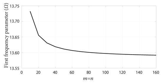
Figure 2. Convergence of the fundamental frequency parameter $\Omega =\omega a^2\sqrt{\rho h/D}$ of a square isotropic plate with $r=0.5$.

Since the results of natural frequency of R–F–R–F plates are limited, the present method was first used to obtain the frequencies of simply supported plates and fully clamped plates. Two boundary conditions have been numerically computed and results are presented in Table 1 and Table 2: (1) two opposite edges ($x=0$ and $x=a$) simply supported and the other two ($y=0$ and $y=b$) free (i.e., S–F–S–F); and (2) two opposite edges ($x=0$ and $x=a$) fully clamped and the other two ($y=0$ and $y=b$) free (i.e., C–F–C–F). As mentioned before, these two cases can be treated as two limit cases with rotational fixity factors, $r=0$ and $r=1$, respectively. It should be noted that $r\ne 1$ in Equation (27) and thus C–F–C–F is simulated by setting $r=0.9999$ in this study. Table 1 tabulates the first six frequency parameters $\Omega =\omega a^2\sqrt{\rho h/D}$ of isotropic plates. Results for orthotropic square plates are illustrated in Table 2. Different aspect ratios were investigated. Excellent agreements can be found from comparisons between the present predictions and previously published results for $r=0$ and $r=0.9999$ (i.e., S–F–S–F and C–F–C–F), respectively. Additionally, results for R–F–R–F plates with $r=0.5$ are also provided for future comparisons.

Table 1. First six frequency parameters $\Omega =\omega a^2\sqrt{\rho h/D}$ for isotropic plates with three different rotational fixity factors ($\nu =0.3$).

r	$\mathit{b}/\mathit{a}$	Results	Mode
			1	2	3	4	5	6
0	0.5	[26]	9.88	27.6	39.48	64.88	88.84	105.56
		[27]	9.87	27.52	39.48	64.54	88.83	105.48
		present	9.5114	27.4730	38.5184	64.4515	87.2662	105.4009
	1	[26]	9.87	16.22	36.82	39.48	47.14	71.33
		[27]	9.87	16.13	36.71	39.48	46.73	70.73
		[28]	9.6314	16.1348	36.7256	38.9450	46.7381	70.7401
		present	9.6296	16.1129	36.6655	38.9360	46.6979	70.6287
	2	[26]	9.87	11.79	17.83	27.91	39.48	41.53
		[27]	9.87	11.66	17.66	27.73	39.48	41.18
		present	9.7340	11.6745	17.6572	27.7048	39.1773	41.1702
0.5	0.5	present	13.5055	29.1960	43.3384	67.5191	92.4649	105.8957
	1	present	13.5969	18.8036	37.9805	43.7159	50.7794	73.4469
	2	present	13.6752	15.1321	20.1497	29.3911	43.4613	43.9340
0.9999	0.5	[26]	22.39	36.46	61.69	83.03	110.9	120.9
		present	22.2067	36.0988	61.2502	82.7627	109.5111	120.3845
	1	[26]	22.39	26.61	44.13	61.69	67.66	80.76
		[28]	22.272	26.529	43.664	61.466	67.549	79.904
		present	22.3421	26.5631	43.7064	61.6519	67.6178	79.8786
	2	[26]	22.39	23.51	27.72	35.96	49.02	61.69
		present	22.4337	23.5357	27.6433	35.6897	48.6187	61.8753

Table 2. First six frequency parameters $\Omega =\omega a^2\sqrt{\rho h/D_x}$ for orthotropic square plates ($b/a=1$) with three different rotational fixity factors.

r	${\mathit{D}}_{\mathit{x}}/{\mathit{D}}_{\mathit{y}}$	$\mathit{H}/{\mathit{D}}_{\mathit{y}}$	${\mathit{\nu }}_{\mathit{x}}$	Results	Mode
					1	2	3	4	5	6
0	0.5	0.5	0.3	[29]	9.1507	13.511	37.46	40.4704	42.3718	68.5419
				present	9.1484	13.4905	37.4421	40.4343	42.3186	68.4430
		1	0.3	[29]	9.3871	20.5731	38.404	50.9914	53.0128	87.1387
				present	9.3835	20.5387	38.3858	50.9049	52.9419	87.0934
		2	0.3	[29]	9.55	29.4576	38.8208	66.6428	67.3417	87.8272
				present	9.5461	29.4211	38.8042	66.5191	67.2802	87.7881
0.5	0.5	2	0.3	present	13.5354	31.0445	43.5971	67.3021	70.2325	92.9605
0.9999	14.5454	0.9644	0.24	[30]	22.369	22.695	24.49	30.2	42.1	60.49
				present	22.5461	22.8694	24.6502	30.3287	42.1714	60.5361

Furthermore, considerable numerical results have been obtained for R–F–R–F orthotropic plates and compared with existing results reported by Liu and Huang [16]. In the work of [16], five different flexural properties and two different aspect ratios were investigated. In particular, three different degrees of rotational restraints were studied, which was described by the parameter of $\Phi =D_x/Ra$. Consequently, the corresponding rotational fixity factor in Equation (5) can be expressed by

$$r=\frac{1}{1+3\Phi }$$

(29)

Extensive comparisons are illustrated in Table 3 and Table 4 and excellent agreement can be observed. However, it can be found that results of [16] for most results of $\Phi =0.1$ are lower than the present results, which were denoted in bold. Such findings were also reported by Liu and Huang in [16] when comparing their results of C–C–C–C and C–C–C–F plates with others.

Table 3. First six frequency parameters $\Omega =\omega a^2\sqrt{\rho h/H}$ for orthotropic plates with various flexural stiffness and different rotational fixity factors ($D_y/H=1$, $\nu =0.3$, and $a/b=1$).

${\mathit{D}}_{\mathit{x}}/\mathit{H}$	$\mathbf{\Phi }$	r	Results	Mode
				1	2	3	4	5	6
1	0.01	0.97087	[16]	21.476	25.914	43.323	59.327	65.800	80.462
			present	21.495	25.712	42.896	59.356	65.331	79.174
	0.1	0.76923	[16]	17.192	21.908	40.141	49.776	56.630	78.336
			present	17.157	21.686	39.721	49.607	56.055	76.882
	10000	0.00003	[16]	9.678	16.302	37.026	39.143	47.228	72.508
			present	9.630	16.113	36.666	38.936	46.698	70.629
1.5	0.01	0.97087	[16]	26.373	30.161	46.075	72.836	78.355	81.195
			present	26.742	30.281	45.946	73.780	78.720	81.058
	0.1	0.76923	[16]	21.112	25.159	42.051	61.145	66.971	78.812
			present	22.501	26.206	42.548	63.752	68.960	78.524
	10000	0.00003	[16]	11.952	17.768	37.700	48.164	55.034	76.631
			present	11.893	17.560	37.324	47.909	54.406	75.520
2	0.01	0.97087	[16]	30.494	33.877	48.647	82.683	84.205	89.170
			present	31.127	34.237	48.733	82.787	85.849	90.154
	0.1	0.76923	[16]	24.428	28.034	43.865	70.707	75.917	79.278
			present	27.062	30.272	45.315	75.934	80.192	80.409
	10000	0.00003	[16]	13.858	19.121	38.362	55.742	61.681	77.413
			present	13.790	18.896	37.971	55.449	61.150	75.842
2.5	0.01	0.97087	[16]	34.120	37.223	51.078	84.182	94.212	98.824
			present	34.971	37.777	51.337	84.426	96.432	100.298
	0.1	0.76923	[16]	27.338	30.640	45.603	79.122	80.206	83.922
			present	31.090	33.962	47.974	81.840	86.763	90.744
	10000	0.00003	[16]	15.532	20.385	39.013	62.406	68.005	76.640
			present	15.455	20.144	38.607	62.080	67.221	76.162
3	0.01	0.97087	[16]	37.396	40.291	53.393	85.647	103.258	107.638
			present	38.433	41.011	53.797	86.002	105.969	109.509
	0.1	0.76923	[16]	29.965	33.040	47.273	81.178	86.745	91.235
			present	34.726	37.349	50.517	83.453	96.588	100.209
	10000	0.00003	[16]	17.012	21.574	39.654	68.423	73.641	76.745
			present	16.958	21.318	39.233	68.068	72.787	76.481
3.5	0.01	0.97087	[16]	40.407	43.141	55.607	87.079	111.564	115.745
			present	41.610	44.007	56.140	87.530	114.720	118.004
	0.1	0.76923	[16]	32.380	35.277	48.884	82.144	93.714	98.015
			present	38.060	40.490	52.951	85.030	105.631	108.976
	10000	0.00003	[16]	18.428	22.701	40.284	73.593	77.026	78.877
			present	18.338	22.432	39.849	73.570	76.799	77.957

Table 4. First six frequency parameters $\Omega =\omega a^2\sqrt{\rho h/H}$ for orthotropic plates with various flexural stiffness and different rotational fixity factors ($D_y/H=1$, $\nu =0.3$, and $a/b=0.5$)).

${\mathit{D}}_{\mathit{x}}/\mathit{H}$	$\mathbf{\Phi }$	r	Results	Mode
				1	2	3	4	5	6
1	0.01	0.97087	[16]	21.357	35.537	58.967	81.294	109.976	115.987
			present	21.366	35.170	58.966	80.416	108.770	115.971
	0.1	0.76923	[16]	17.094	31.760	49.427	72.700	100.455	107.749
			present	17.060	31.389	49.249	71.823	100.058	106.691
	10000	0.00003	[16]	9.570	27.810	38.712	65.210	87.729	106.456
			present	9.512	27.473	38.519	64.452	87.266	105.401
1.5	0.01	0.97087	[16]	26.279	38.807	72.541	91.761	111.206	142.856
			present	26.637	38.797	73.461	91.802	110.322	144.289
	0.1	0.76923	[16]	21.051	34.121	60.857	81.023	108.491	123.765
			present	22.418	34.861	63.462	82.477	107.974	127.221
	10000	0.00003	[16]	11.866	28.692	47.810	71.071	106.570	108.108
			present	11.798	28.346	47.571	70.237	105.632	107.520
2	0.01	0.97087	[16]	30.412	41.798	83.941	101.146	112.381	165.514
			present	31.037	42.042	85.572	101.866	111.714	167.983
	0.1	0.76923	[16]	24.370	36.315	70.446	88.559	109.239	143.418
			present	26.989	38.162	75.681	92.409	109.298	150.643
	10000	0.00003	[16]	13.753	29.538	55.431	76.482	106.800	125.350
			present	13.707	29.192	55.157	75.582	105.862	124.522
2.5	0.01	0.97087	[16]	34.046	44.576	93.972	109.733	113.520	184.433
			present	34.890	45.022	96.185	110.996	113.017	175.721
	0.1	0.76923	[16]	27.268	38.364	78.885	95.905	109.972	160.741
			present	31.022	41.261	86.535	101.642	110.610	167.809
	10000	0.00003	[16]	15.439	30.372	62.126	81.537	107.033	140.538
			present	15.382	30.015	61.819	80.572	106.092	139.466
3	0.01	0.97087	[16]	37.329	47.184	103.032	114.635	117.697	193.554
			present	38.361	47.801	105.744	114.263	119.417	181.325
	0.1	0.76923	[16]	29.901	40.317	86.506	101.984	110.698	175.531
			present	34.663	44.176	96.379	110.262	111.896	173.447
	10000	0.00003	[16]	16.956	31.180	68.166	86.296	107.266	154.272
			present	16.891	30.816	67.830	85.271	106.321	152.957
3.5	0.01	0.97087	[16]	40.345	49.653	111.351	115.728	125.250	190.216
			present	41.543	50.418	114.511	115.467	127.275	186.716
	0.1	0.76923	[16]	32.326	42.179	93.507	108.072	111.416	183.912
			present	38.001	46.927	105.437	113.152	118.355	178.938
	10000	0.00003	[16]	18.353	31.977	73.713	90.806	107.501	166.512
			present	18.277	31.596	73.350	89.725	106.550	159.394

At last, the influence of different degrees of rotational restraints on the mode shapes was investigated. Figure 3 shows the first, second and third mode shapes of R–F–R–F orthotropic square plates with three different values of rotational fixity factors (0, 0.5 and 0.9999). The mode shapes can be found to be significantly altered by the rotational restraints.

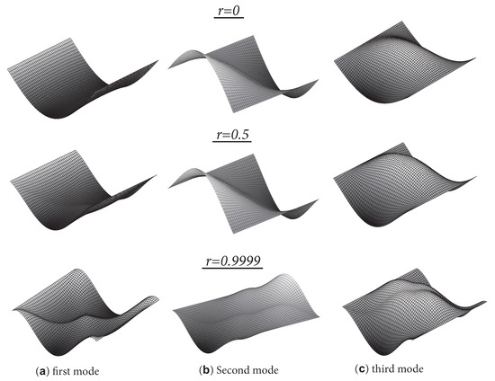
Figure 3. Mode shapes of a square orthotropic plate with different rotational restraints. (a) first mode; (b) second mode; (c) third mode.

4. Conclusions

In the present paper, an exact series solution for free vibration of a rectangular orthotropic plate with opposite rotationally restrained and free edges was obtained by using the finite integral transform method. A new alternative formulation was developed for the application of such a method to the transverse vibration of plates. In contrast to the formulation used for the flexural deformation of plates, a much easier eigenvalue solution can be obtained without solving a highly non-linear equation. Extensive numerical studies have been conducted to validate the present method for plates with different structural properties, rotational restraints and aspect ratios. Comparisons with existing results indicate excellent accuracy and efficiency of the present method. The mode shapes are found to be altered significantly by the rotational restraints. The merits of the present method are that the method is simple and straightforward and can be calculated with the desired accuracy.

References

- Leissa, A.W. Vibration of Plates; NASA SP-160; National Aeronautics and Space Administration: Washington, DC, USA, 1969. [Google Scholar]
- Soedel, W. Vibrations of Shells and Plates; CRC Press: Boca Raton, FL, USA, 2004. [Google Scholar]
- Szilard, R. Theories and Applications of Plate Analysis: Classical, Numerical and Engineering Methods; John Wiley & Sons: Hoboken, NJ, USA, 2004. [Google Scholar]
- Wang, C.Y.; Wang, C.M. Structural Vibration: Exact Solutions for Strings, Membranes, Beams, and Plates; CRC Press: Boca Raton, FL, USA, 2016. [Google Scholar]
- Hoppmann, W.H., II; Greenspon, J. Flexural Vibration of a Plate with Elastic Rotational Constraint on Boundary; Technical Report 8; Department of Mechanical Engineering, The Johns Hopkins University: Baltimore, MD, USA, 1953. [Google Scholar]
- Carmichael, T. The vibration of a rectangular plate with edges elastically restrained against rotation. Q. J. Mech. Appl. Math. 1959, 12, 29–42. [Google Scholar] [CrossRef]
- Laura, P.; Luisoni, L.; Filipich, C. A note on the determination of the fundamental frequency of vibration of thin, rectangular plates with edges possessing different rotational flexibility coefficients. J. Sound Vib. 1977, 55, 327–333. [Google Scholar] [CrossRef]
- Mukhopadhyay, M. Free vibration of rectangular plates with edges having different degrees of rotational restraint. J. Sound Vib. 1979, 67, 459–468. [Google Scholar] [CrossRef]
- Laura, P.; Grossi, R. Transverse vibrations of rectangular plates with edges elastically restrained against translation and rotation. J. Sound Vib. 1981, 75, 101–107. [Google Scholar] [CrossRef]
- Warburton, G.; Edney, S. Vibrations of rectangular plates with elastically restrained edges. J. Sound Vib. 1984, 95, 537–552. [Google Scholar] [CrossRef]
- Zhou, D. An approximate solution of eigen-frequencies of transverse vibration of rectangular plates with elastical restraints. Appl. Math. Mech. 1996, 17, 451–456. [Google Scholar]
- Laura, P.; Grossi, R. Transverse vibration of a rectangular plate elastically restrained against rotation along three edges and free on the fourth edge. J. Sound Vib. 1978, 59, 355–368. [Google Scholar] [CrossRef]
- Grossi, R.; Laura, P. Transverse vibrations of rectangular orthotropic plates with one or two free edges while the remaining are elastically restrained against rotation. Ocean Eng. 1979, 6, 527–539. [Google Scholar] [CrossRef]
- de Irassar, P.V.; Ficcadenti, G.; Laura, P. Transverse vibrations of rectangular orthotropic plates with the edges elastically restrained against rotation and a free, straight corner cut-out. Fibre Sci. Technol. 1982, 16, 247–259. [Google Scholar] [CrossRef]
- Grace, N.F.; Kennedy, J.B. Dynamic analysis of orthotropic plate structures. J. Eng. Mech. 1985, 111, 1027–1037. [Google Scholar] [CrossRef]
- Liu, W.; Huang, C.C. Free vibration of a rectangular plate with elastically restrained and free edges. J. Sound Vib. 1987, 119, 177–182. [Google Scholar] [CrossRef]
- Li, R.; Zhong, Y.; Tian, B.; Liu, Y. On the finite integral transform method for exact bending solutions of fully clamped orthotropic rectangular thin plates. Appl. Math. Lett. 2009, 22, 1821–1827. [Google Scholar] [CrossRef]
- Tian, B.; Zhong, Y.; Li, R. Analytic bending solutions of rectangular cantilever thin plates. Arch. Civ. Mech. Eng. 2011, 11, 1043–1052. [Google Scholar] [CrossRef]
- Li, R.; Tian, B.; Zhong, Y. Analytical bending solutions of free orthotropic rectangular thin plates under arbitrary loading. Meccanica 2013, 48, 2497–2510. [Google Scholar] [CrossRef]
- An, C.; Gu, J.; Su, J. Exact solution of bending problem of clamped orthotropic rectangular thin plates. J. Braz. Soc. Mech. Sci. Eng. 2016, 38, 601–607. [Google Scholar] [CrossRef]
- Zhang, S.; Xu, L. Bending of rectangular orthotropic thin plates with rotationally restrained edges: A finite integral transform solution. Appl. Math. Model. 2017, 46, 48–62. [Google Scholar] [CrossRef]
- Zhang, S.; Xu, L. Analytical solutions for flexure of rectangular orthotropic plates with opposite rotationally restrained and free edges. Arch. Civ. Mech. Eng. 2018, 18, 965–972. [Google Scholar] [CrossRef]
- Zhang, S. Vibration Serviceability of Cold-Formed Steel Floor Systems. Ph.D. Thesis, University of Waterloo, Waterloo, ON, Canada, 2017. [Google Scholar]
- Sneddon, I. The Use of Integral Transforms; McGraw-Hill, Inc.: New York, NY, USA, 1972. [Google Scholar]
- Khalili, M.R.; Malekzadeh, K.; Mittal, R. A new approach to static and dynamic analysis of composite plates with different boundary conditions. Compos. Struct. 2005, 69, 149–155. [Google Scholar] [CrossRef]
- Warburton, G.B. The vibration of rectangular plates. Proc. Inst. Mech. Eng. 1954, 168, 371–384. [Google Scholar] [CrossRef]
- Jankovic, V. The Solution of the Frequency Equation of Plates Using Digital Computers. Stavebnícky Čas. 1964, 12, 360–365. (In Czech) [Google Scholar]
- Leissa, A.W. The free vibration of rectangular plates. J. Sound Vib. 1973, 31, 257–293. [Google Scholar] [CrossRef]
- Jayaraman, G.; Chen, P.; Snyder, V. Free vibrations of rectangular orthotropic plates with a pair of parallel edges simply supported. Comput. Struct. 1990, 34, 203–214. [Google Scholar] [CrossRef]
- Bassily, S.F.; Dickinson, S.M. Comment on “Free Vibrations of Generally Orthotropic Plates”. J. Acoust. Soc. Am. 1972, 52, 1050–1053. [Google Scholar] [CrossRef]
© 2018 by the authors. Licensee MDPI, Basel, Switzerland. This article is an open access article distributed under the terms and conditions of the Creative Commons Attribution (CC BY) license (http://creativecommons.org/licenses/by/4.0/).