Article

Surface-Wave Extraction Based on Morphological Diversity of Seismic Events

1
School of Geophysics and Information Technology, China University of Geosciences (Beijing), Beijing 100083, China
2
The State Key Laboratory of Ore Deposit Geochemistry, Institute of Geochemistry, Chinese Academy of Sciences, Guiyang 550081, China
3
Key Laboratory of Marine Reservoir Evolution and Hydrocarbon Accumulation Mechanism, Ministry of Education, China University of Geosciences (Beijing), Beijing 100083, China
*
Author to whom correspondence should be addressed.
Appl. Sci. 2019, 9(1), 17; https://doi.org/10.3390/app9010017
Submission received: 14 October 2018 / Revised: 18 December 2018 / Accepted: 19 December 2018 / Published: 21 December 2018
(This article belongs to the Special Issue Seismic Metamaterials)

Abstract

:

Featured Application

The proposed method is applicable for surface-wave extraction on X component in multicomponent seismic exploration. This method has application potential for the separation of PS-waves and surface waves whose frequencies and velocities are close.

Abstract

It is essential to extract high-fidelity surface waves in surface-wave surveys. Because reflections usually interfere with surface waves on X components in multicomponent seismic exploration, it is difficult to extract dispersion curves of surface waves. To make matters worse, the frequencies and velocities of higher-mode surface waves are close to those of PS-waves. A method for surface-wave extraction is proposed based on the morphological differences between surface waves and reflections. Frequency-domain high-resolution linear Radon transform (LRT) and time-domain high-resolution hyperbolic Radon transform (HRT) are used to represent surface waves and reflections, respectively. Then, a sparse representation problem based on morphological component analysis (MCA) is built and optimally solved to obtain high-fidelity surface waves. An advantage of our method is its ability to extract surface waves when their frequencies and velocities are close to those of reflections. Furthermore, the results of synthetic and field examples confirm that the proposed method can attenuate the distortion of surface-wave dispersive energy caused by reflections, which contributes to extraction of accurate dispersion curves.

1. Introduction

Seismic surface waves are widely used in crustal and mantle structure studies as well as engineering prospecting. They are characterized by low attenuation with offset, a high signal-to-noise ratio, and dispersion [1,2]. The dispersion characteristics of surface waves reflect the near-surface S-wave velocity structure. Dispersion curves of fundamental-mode surface waves are inverted to obtain a near-surface S-wave velocity structure for PS-wave static corrections in seismic exploration [3,4]. Recently, some studies have found that fundamental- and higher-mode surface waves have different sensitivities to elastic properties and thicknesses of near-surface materials [5,6]. Thus, joint inversion of fundamental- and higher-mode surface waves is of widespread interest for less ambiguity and higher accuracy of S-wave velocities in engineering seismic prospecting, ambient seismic noise tomography, and microtremor surveys [7,8]. To obtain accurate S-wave velocities, extraction of accurate dispersion curves of multi-mode surface waves is essential.
Fundamental-mode surface waves are dominant in vertical-component seismic data, while higher-mode surface waves are generally more evident on horizontal components or X components in two-dimensional (2D) surveys [9]. Because they are disturbed by reflections, it is usually difficult to extract accurate dispersion curves of higher-mode surface waves from X-component seismic data, causing ambiguity in the inverted S-wave velocities. Luo et al. [10] propose high-resolution linear Radon transform (LRT) to image the surface-wave dispersive energy, which improves the resolution of phase velocities. However, when disturbed by body waves or strong noise, the dispersive energy may not be smooth, and, thus, it becomes hard to distinguish between different modes; this is known as “mode kissing” [11]. This phenomenon is vulnerable to mode misidentification [12], resulting in less reliable inversion or even wrong inverted S-wave velocities.
To extract dispersion curves, surface waves are extracted on the basis of different characteristics between surface waves and interference waves. Methods of surface-wave suppression are based on single-component processing or multicomponent processing. Methods of single-component processing include f-k filtering, curvelet transform, and other transform methods [13,14,15], while methods of multicomponent processing are polarization filtering and vector median filtering, which preserve the vector characteristics and the spectral bandwidth of reflections [16,17]. By a hybrid linear-hyperbolic Radon transform, Trad et al. [18] separate surface waves successfully in a signal model that consists of both surface waves with linear events and reflections with hyperbolic events. However, raw data are transformed into the conventional intercept-slowness (τ-p) domain, which is not sparse enough to separate surface waves according to their dispersion characteristics. Using high-resolution LRT, Hu et al. [19] transform raw data into the frequency-velocity (f-v) domain to implement surface-wave separation. However, dispersive energy of higher-mode surface waves may overlap with that of reflections in the f-v domain, because the frequencies and velocities of PS-waves are close to those of higher-mode surface waves [16]. So, it may be difficult to extract surface waves from X-component seismic data.
In this paper, we propose a method of surface-wave extraction to overcome the influence of reflections on surface-wave dispersive energy. The proposed method is based on the morphological differences between surface waves and reflections. We also exploit the advantages of wavefield separation by frequency-domain LRT and time-domain hyperbolic Radon transform (HRT). To implement surface-wave extraction, the sparse representation problem based on morphological component analysis (MCA) is optimally solved.
We first describe the sparse representation problem and the selection of dictionaries. Next, we demonstrate the distortion of surface-wave dispersive energy caused by reflections. Then, we demonstrate the results of surface-wave extraction and dispersion curves using tests with synthetic and field shot data.

2. Conventional Method: Extracting Surface Waves in the f-v Domain

High-resolution LRT is used to image surface-wave dispersive energy [10]. Using this, surface waves and reflections on Z components are present clearly in different locations of the f-v domain when their frequencies and velocities are significantly different. Hu et al. [19] extract surface waves from Z components by a 2D window of the f-v domain.
The frequency-domain inverse LRT in the matrix-vector form is [18]:
d ( f ) = L ( f ) m ( f )
where d ( f ) is a vector of size n x × 1 representing the Fourier coefficients of the seismic data at the given frequency f , while m ( f ) is a vector of size n p × 1 representing the Fourier coefficients of the Radon panel at the given frequency f . In Equation (1), L ( f ) is a complex matrix of size n x × n p :
L ( f ) = [ e i 2 π f x 1 v 1 e i 2 π f x 1 v 2 e i 2 π f x 1 v n p e i 2 π f x 2 v 1 e i 2 π f x 2 v 2 e i 2 π f x 2 v n p e i 2 π f x n x v 1 e i 2 π f x n x v 2 e i 2 π f x n x v n p ]
where v i ( i = 1 , 2 , , n p ) is the apparent velocity and x j ( j = 1 , 2 , , n x ) is the offset.
The frequency-domain high-resolution forward LRT [20,21] is inverted with a sparse constraint of a priori probability, known as:
( λ I + W m H L H W d H W d L W m 1 ) m ˜ = W m H L H W d H W d d
where m ˜ = W m m . W d is a matrix of data weights, specifically, a diagonal matrix showing the standard deviation, diag ( W d ) i = | ( d - L m ) i | 1 / 2 , while W m is a diagonal matrix of Radon coefficients indicating how sparse the coefficients are, diag ( W m ) i = | m i | 1 / 2 . I is the identity matrix, and the scalar λ is the tradeoff parameter that weights the relative levels of importance of the misfit and the sparsity [22].
However, it is difficult to extract surface waves correctly from X-component seismic data, because the frequencies and velocities of higher-mode surface waves and PS-waves are close and both of them are generally evident on X components. Disturbed by PS-waves, the dispersive energy is not true for surface waves. So, extracting surface waves in the f-v domain is not a perfect method. We propose a method of surface-wave extraction based on MCA to avoid the overlaps between surface waves and reflections in the f-v domain. High-resolution LRT is one of two transforms and is used to represent surface waves.

3. New Method: Sparse Representations of Wavefields Based on MCA

MCA is a method for signal separation based on sparse representations [23,24]. It is assumed that the original signal is a linear mixture of several different parts and for each of them, there exists a dictionary that enables its construction using a sparse representation. Additionally, the dictionary can only sparsely represent the corresponding part rather than the others. For seismic data consisting of surface waves and reflections, there is
y = y g + y r
where y is the seismic data set, y g is the surface-wave part, and y r is the reflection part. We choose D g and D r as the sparse representation dictionaries of surface waves and reflections, respectively, i.e., y g = D g z g , y r = D r z r . The separation of surface waves and reflections can be formulated as [25]:
argmin { z g , z r } 1 2 y D g z g D r z r 2 2 + μ ( z g 1 + z r 1 )
where z g and z r are the representation vectors for the surface waves and reflections, respectively, and μ is the regularization parameter.
Surface waves are generally modeled as broom-like events characterized by low frequency, low velocity, and dispersion. In addition, their dispersive energy is around theoretical dispersion curves in the f-v domain [19,20]. Therefore, frequency-domain high-resolution LRT can, in theory, sparsely represent surface waves. Reflections are approximated by hyperbolas, and time-domain high-resolution HRT can sparsely represent reflections with the assumptions that velocities change little horizontally and reflection interfaces are almost horizontal [26]. We choose frequency-domain high-resolution LRT and time-domain high-resolution HRT to represent surface waves and reflections, respectively. To match with the matrix definition of sparse representation dictionaries in our sparse representation problem, the inverse LRT and inverse HRT correspond to the matrix signs D g and D r , respectively, while the forward LRT and forward HRT are respectively the matrices D g + and D r + . The matrices D g + and D r + are the pseudo inverse of the representation dictionaries, i.e., z g = D g + y g , z r = D r + y r . By putting z g = D g + y g and z r = D r + y r into (5), we obtain
argmin { y g , y r } 1 2 y y g y r 2 2 + μ ( D g + y g 1 + D r + y r 1 )
which is solved by the generalized block coordinate relaxation algorithm [23].
Surface waves are extracted by solving Equation (6). Different dictionaries respectively represent surface waves and reflections so that the influence of reflections on surface-wave dispersive energy is reduced.

3.1. Frequency-Domain High-Resolution LRT

To sparsely represent surface waves, Equation (3) is solved to achieve high-resolution LRT in the spectral bandwidth of surface waves by the iteratively reweighted least squares (IRLS) algorithm [27]. The interval of apparent velocities should be small to avoid aliasing for reconstruction; moreover, the apparent-velocity range includes the phase velocities of surface waves.

3.2. Time-Domain High-Resolution HRT

Inverse and adjoint HRT in the discrete form can be expressed as [21]:
d ( t , x ) = v m ( τ = t 2 x 2 / v 2 , v )
and
m adj ( τ , v ) = x d ( t = τ 2 + x 2 / v 2 , x )
where d ( t , x ) are the seismic data in the time-offset domain, x is the offset, t is two-way time, m ( τ , v ) are the Radon coefficients, v is the root-mean-square velocity of a reflection, τ is the time intercept, and m adj ( τ , v ) are the low-resolution Radon coefficients. Equations (7) and (8) are represented in matrix-vector form as follows [28]:
d = L m
m adj = L T d
where d is a vector of size N × 1 , whose elements are taken trace-wise from the seismic data ( N = n x × n t ), and m is a vector of size M × 1 , whose elements are taken velocity-wise from the Radon coefficients ( M = n v × n τ ). n x , n t , n v , and n τ are the numbers of traces, samples, velocities, and time intercepts, respectively. In Equations (9) and (10), the operators L and L T are just represented for the summation algorithms shown in Equations (7) and (8), instead of matrices [28].
High-resolution forward HRT can be inverted from Equation (9) using a sparse constraint satisfying
( W m T W m ) 1 L T W d T W d L m = ( W m T W m ) 1 L T W d T W d d
which is solved by the algorithm of a left preconditioned version of conjugate gradient for the normal Equations [28].
The computational cost of applying operators L and L T is controlled by the size of the Radon domain [29]. To speed up the implementation, time-domain high-resolution forward HRT is solved in the restricted Radon space [29]
( W m A T W m A ) 1 L A T W d T W d L A m A = ( W m A T W m A ) 1 L A T W d T W d d
where d should be normalized to unity by dividing the maximum of the seismic data [30]. The restricted Radon space is defined as
A = { ( τ , p ) : 1 n x | m adj | > T }
where T is the threshold satisfying 0 < T < 1 .

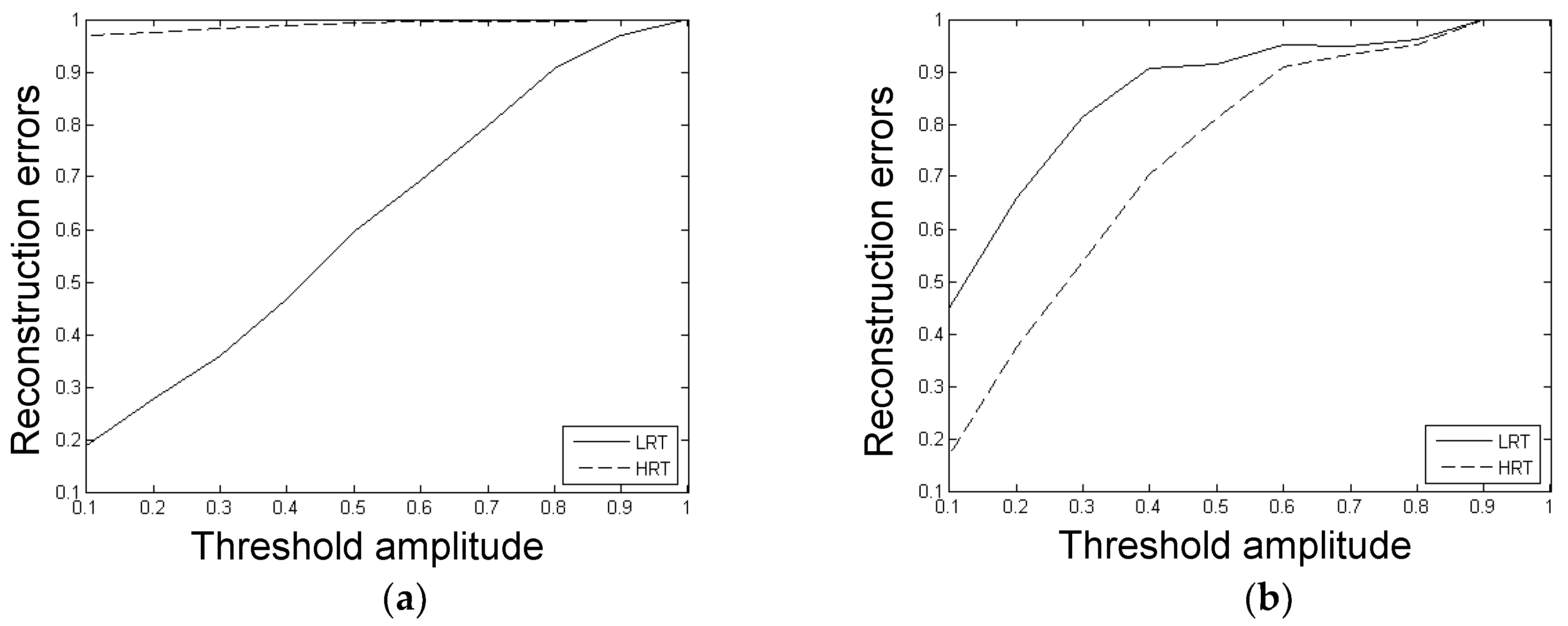
3.3. Performance of Sparse Representations Using LRT and HRT

We synthesize the surface waves (Figure 1) of the two-horizontal-layer model (Model 1) described by Table 1 using the staggered-grid finite-difference method [31]. Then, we synthesize reflections (Figure 2) of the three-horizontal-layer model (Model 2) described by Table 2 using ray tracing. Frequency-domain high-resolution forward LRT and time-domain high-resolution forward HRT are applied to the surface waves and reflections to obtain the four panels of the Radon coefficients. Next, we respectively normalize the Radon coefficients to unity divided by the maximum of each panel and apply hard thresholds to them. Finally, the seismic data were reconstructed by the inverse transforms. For a Radon panel, the higher threshold amplitude means that fewer Radon coefficients are used in the reconstruction.
To confirm the effectiveness of sparse representations for surface waves and reflections, the reconstruction error is calculated as follows:
e r r = x E x r / x E x 0
where E x r is the root-mean-square error between the reconstruction and the original data at the offset x , and E x 0 is the root-mean-square value of the original data at the offset x , and
E x r = 1 n t t ( d ( t , x ) d ˜ ( t , x ) ) 2
E x 0 = 1 n t t ( d ( t , x ) ) 2
where d ˜ ( t , x ) is the reconstruction data. The reconstruction errors against the threshold amplitude are illustrated in Figure 3. According to Figure 3a, fewer coefficients can be used to reconstruct the surface waves by frequency-domain high-resolution LRT compared with time-domain high-resolution HRT, which means the former can represent surface waves more sparsely. On the basis of Figure 3b, time-domain high-resolution HRT can represent reflections more sparsely than frequency-domain high-resolution LRT. Comparing the HRT-reconstruction errors shown by dashed lines between Figure 3a,b, time-domain high-resolution HRT leads to a non-sparse representation for surface waves. Similarly, frequency-domain high-resolution LRT leads to a non-sparse representation for reflections when comparing the LRT-reconstruction errors. Thus, the two transforms (dictionaries) are significantly different in the sparse representations for surface waves and reflections, which meets the assumptions of MCA, and it is theoretically feasible to extract the surface waves based on Equation (6).

4. Examples

4.1. Synthetic Examples

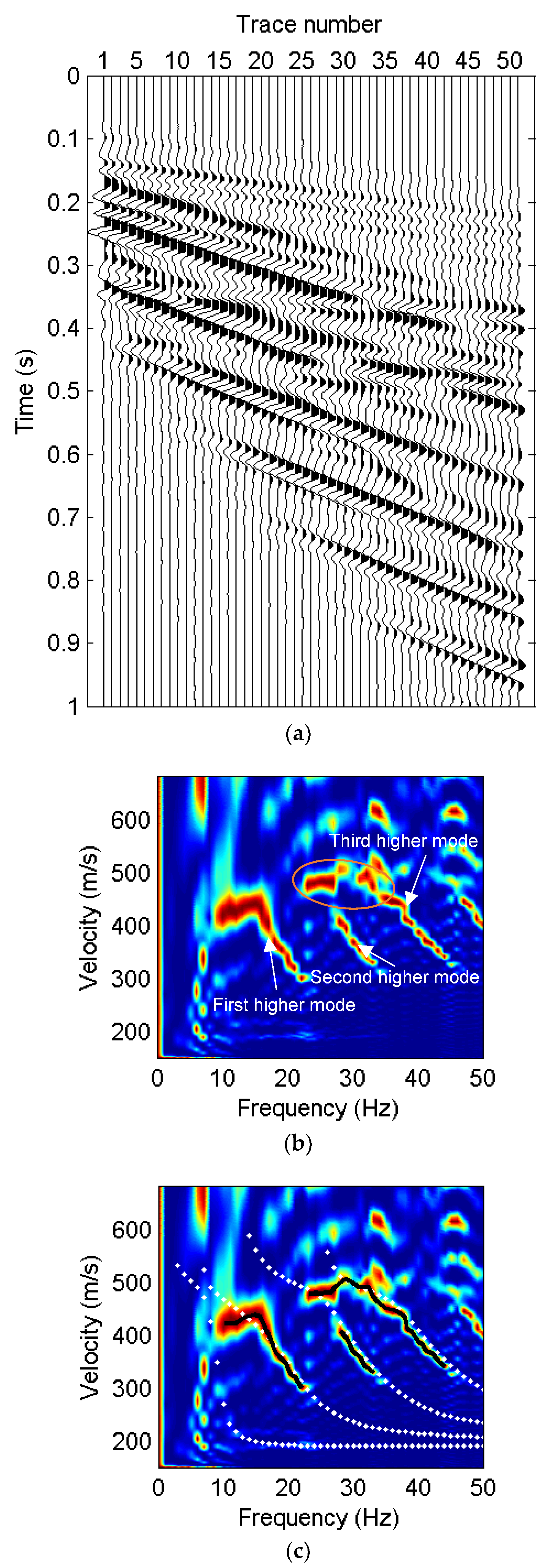
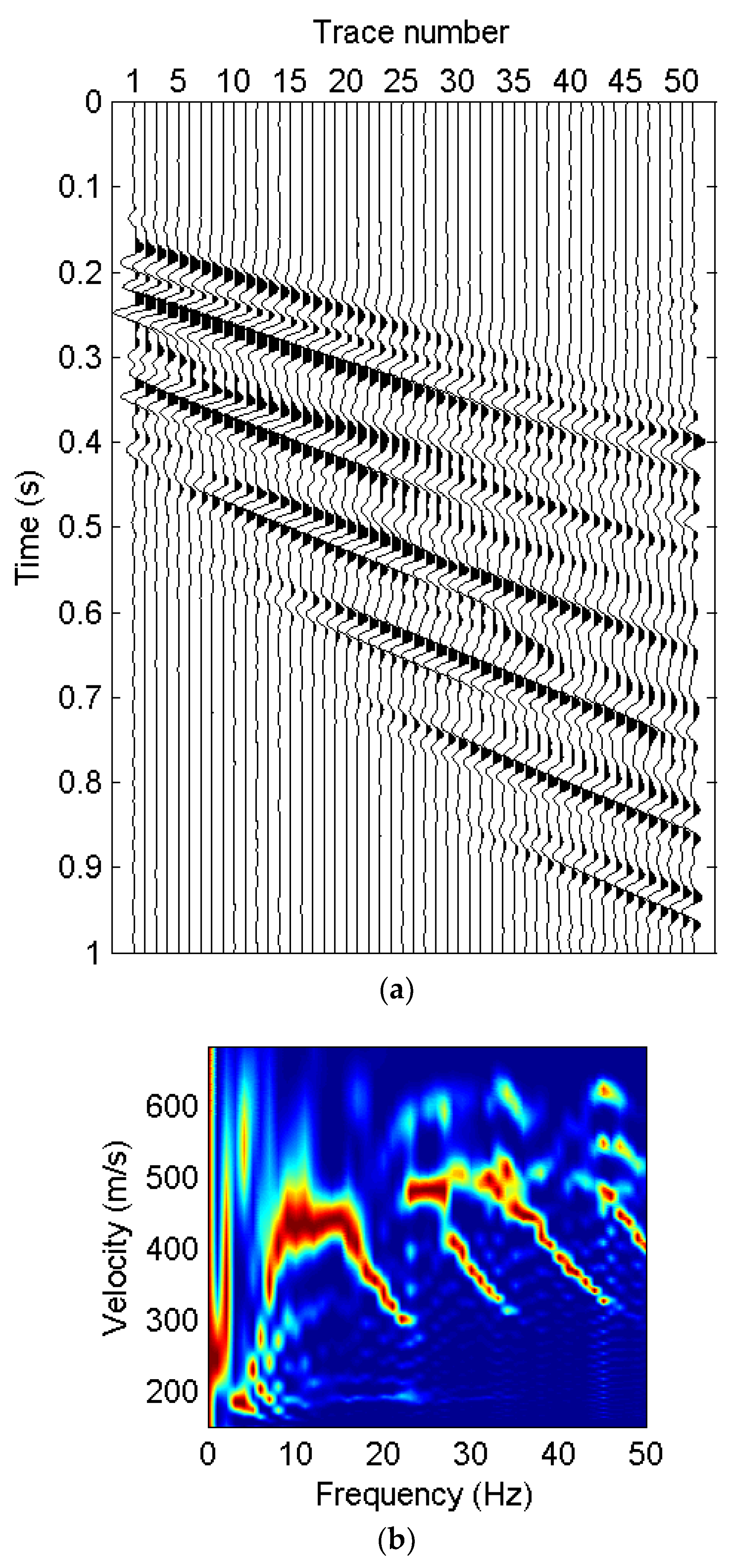
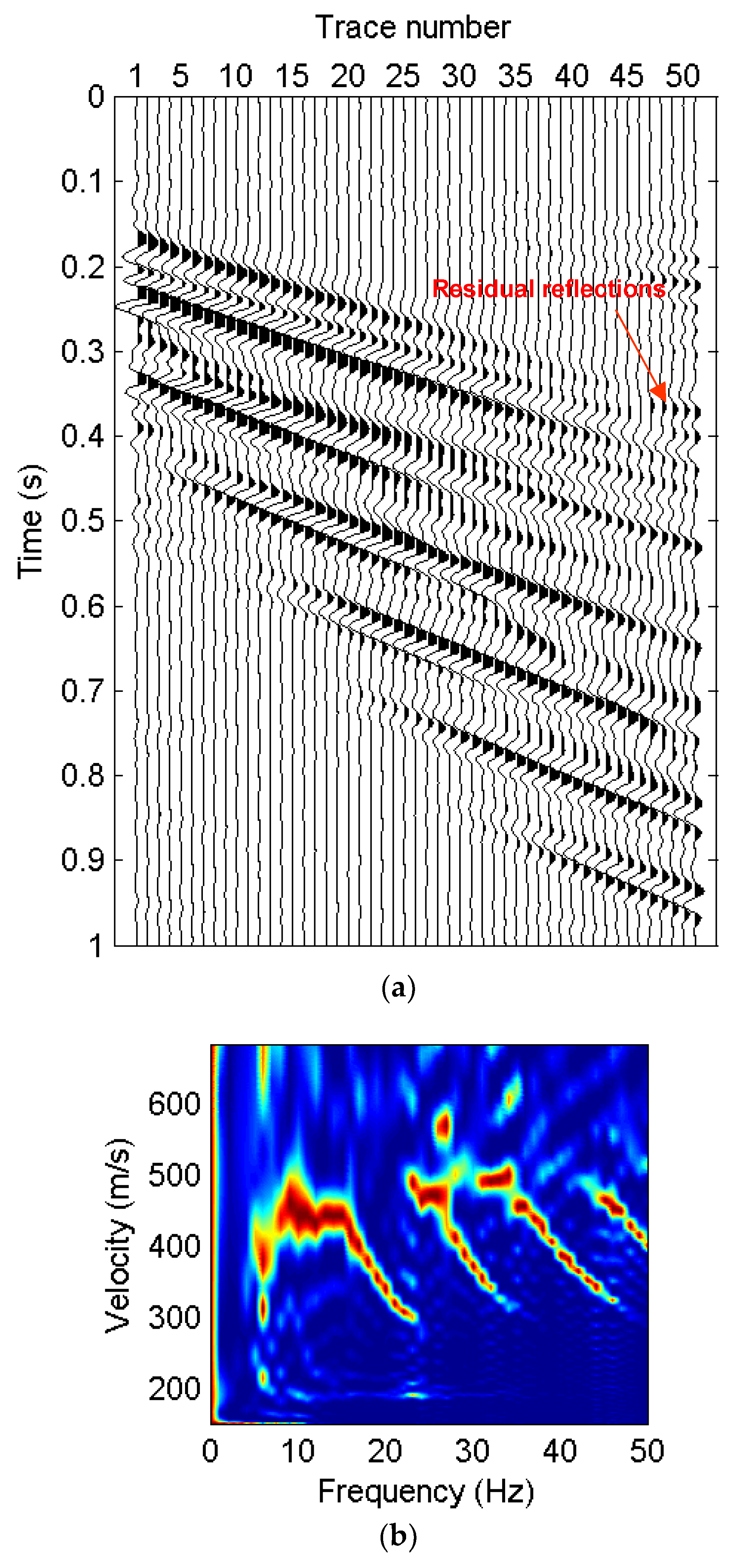
4.1.1. Distortion of Surface-Wave Dispersive Energy Caused by Reflections

The dispersive energy of surface waves can help us to pick dispersion curves. In addition, dispersion curves of surface waves can be inverted to obtain a near-surface S-wave velocity structure for PS-wave static corrections in seismic exploration [3,4]. However, the dispersive energy of higher-mode surface waves may be influenced by reflections in X-component seismic data.
Two layered earth models (Model 3 and Model 4) are given in Table 3 and Table 4 to display the distortion of surface-wave dispersive energy caused by reflections. The layers of Model 3 are the first two layers of Model 4. A synthetic X-component shot gather (Figure 4a) of Model 3 is simulated using a staggered-grid finite-difference method [31] with an explosive source located at a 3-m depth. Another synthetic X-component shot gather (Figure 5a) of Model 4 is simulated using the same method and the same forward-simulation parameters. We simulate the records with 51 receivers evenly spaced (2 m) in line on the surface and the nearest offset of 40 m. As shown in Figure 4b and Figure 5b, the two shot gathers are transformed into the f-v domain by high-resolution LRT.
According to the relationship between penetration depths of Rayleigh waves and wavelengths [32], the surface waves of Model 3 and Model 4 cannot penetrate to a depth of 100 m, so the dispersion characteristics of pure surface waves in Figure 5a should be similar to those in Figure 4a. The surface waves shown in Figure 4a are not disturbed by the reflections from the deep reflectors. The dispersive energy shown in Figure 4b is continuous, and the three branches of dispersion energy clearly correspond to the first, second, and third higher modes. However, the events of the higher-mode surface waves in Figure 5a discontinuously overlap with the reflections in the two-way time of 0.35 s and 0.45 s. In addition, it is difficult to discern whether the dispersive energy, at frequencies of 25–33 Hz and apparent velocities of 470–530 m/s (energy circled in Figure 5b), corresponds to the second higher mode or the third higher mode. A comparison of Figure 4b and Figure 5b demonstrates that reflections may disturb the dispersive energy of surface waves. What causes this phenomenon, “mode kissing”, is the non-negligible effect of the reflections within this range of frequencies and velocities. The picked dispersion curves based on the amplitude and the continuity of dispersive energy are shown in Figure 5c, where the second higher mode of frequencies of 25–27 Hz is misidentified as the third higher mode. However, the surface-wave dispersive energy on Z-component seismic data is not severely influenced by the reflections from the deep reflectors according to Hu et al. [19].

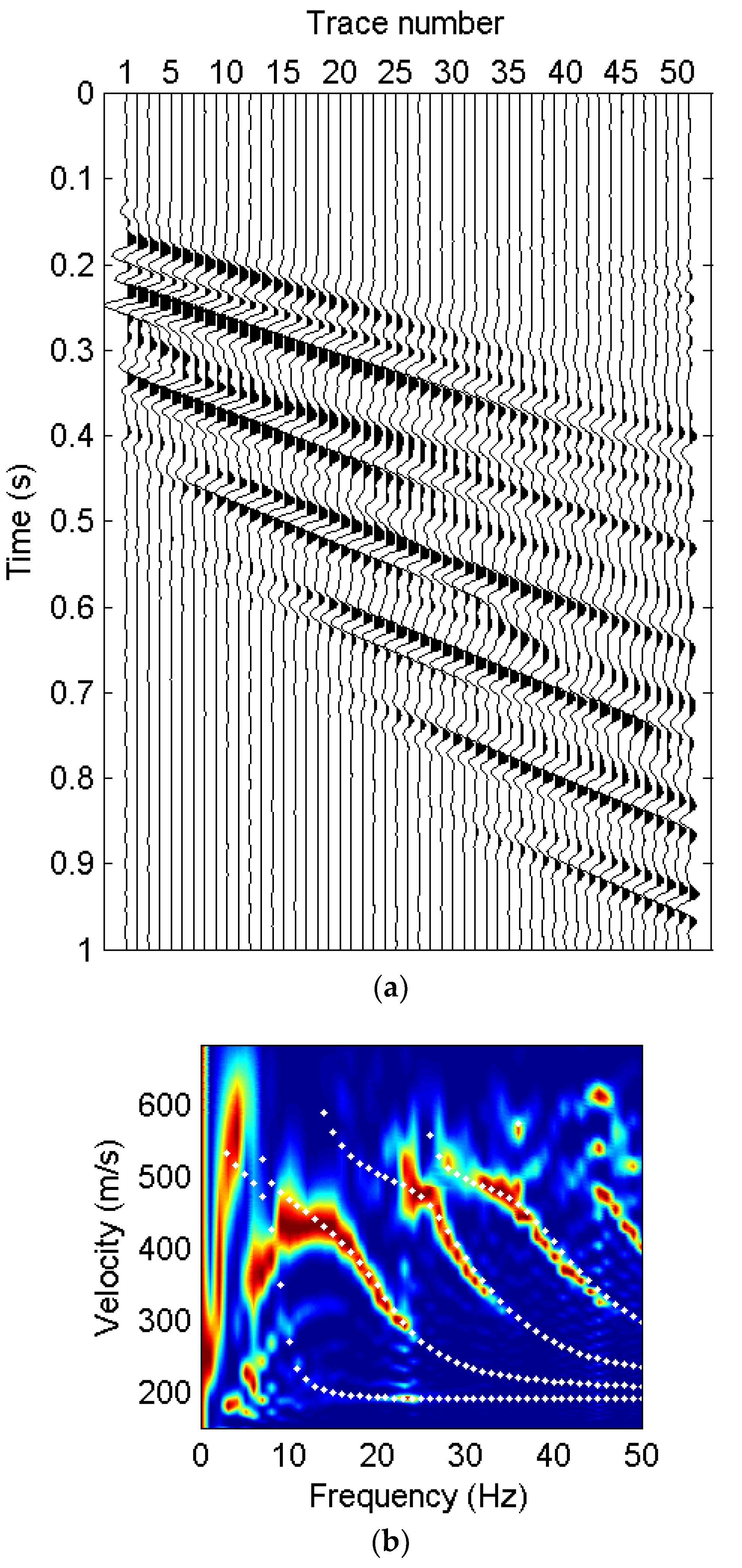
4.1.2. Recovery of the Surface-Wave Dispersive Energy
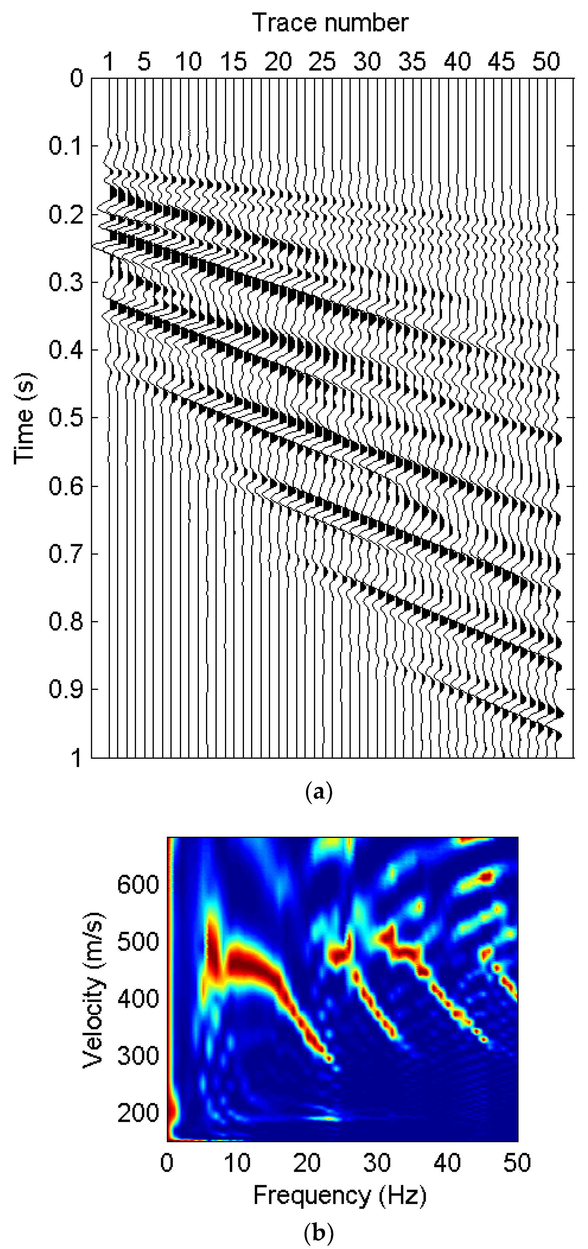
The proposed method is applied to the synthetic seismic data shown in Figure 5a to display the results of surface-wave extraction and the improvement of the surface-wave dispersive energy. Compared with the dispersive energy of the original seismic data shown in Figure 5b, the dispersive energy of the surface waves extracted from the data is more continuous in Figure 6. The energy at frequencies of 25–27 Hz and 28–33 Hz is separated into two parts corresponding to the second higher mode and the third higher mode, respectively, which means that “mode kissing” disappears. Additionally, the dispersive energy is close to the theoretical dispersion curves, which implies that surface waves can be effectively extracted using the proposed method.
Furthermore, we compare the proposed method with other methods of surface-wave extraction to test the superiority of the proposed method. High-resolution LRT is applied to the original data and a 2D window is used to select and extract surface waves in the f-v domain. Figure 7 shows that the surface waves are mainly extracted but “mode kissing” is not changed. The f-k filtering method is also used to extract surface waves. The result of the surface-wave extraction consists of residual reflections in Figure 8a and “mode kissing” is reduced in Figure 8b. However, there is also a risk of mode misidentification owing to the discontinuous dispersive energy shown in Figure 8b.

4.2. Field Example

The X-component field data of 2D3C seismic data shown in Figure 9 were acquired in Wangjiatun District, Daqing Oilfield, China with a sample interval of 4 ms, a geophone interval of 25 m, and a nearest offset of 400 m. It can be seen that several events of higher-mode surface waves overlap with the reflections. The surface waves are mainly at the range of low frequencies and low velocities, while reflections are in the whole f-v domain (Figure 10). Several branches of dispersive energy at frequencies of ~5 Hz and velocities of 800–1000 m/s, circled in Figure 10, are very close to each other, resulting in inaccurate phase velocities at those frequencies. The extracted surface waves extracted by the proposed method are shown in Figure 11a, where most of surface waves are extracted, and the rest of the field data are reflections and other noises, except for a small number of surface waves (circled in Figure 11b). This is because the morphologies of the surface waves and reflections are slightly distorted by diffraction waves and other noises. These noises are caused by small-size geological subjects (pinch-outs or fractures) [33].
To display the effectiveness of surface-wave extraction further, the details of waveforms are compared in Figure 12, where the original field data (Figure 9) and the results of surface-wave extraction (Figure 11a) in section A and section B are magnified. For section A, the original data (Figure 12a) are dominated by reflections, while the events of surface waves can be clearly identified in the results of surface-wave extraction (Figure 12b). For section B, the events of surface waves (Figure 12d) are clearer and more continuous than those before surface-wave extraction (Figure 12c). The image of dispersive energy of the extracted surface waves using the proposed method is shown in Figure 13a. After surface-wave extraction, the dispersive energy of different modes is separated, and the ambiguity of the phase velocities in Figure 10 is eliminated. As shown in Figure 13b, we can easily pick dispersion curves from Figure 13a. For comparison, the dispersive energy of surface waves separated by the f-k filtering method is displayed in Figure 14, where it is difficult to identify the modes of dispersive energy at frequencies of 4.5–7 Hz and velocities of 850–1100 m/s. The results of the synthetic example and the field example demonstrate that surface-wave extraction by the proposed method attenuates the distortion of the surface-wave dispersive energy caused by reflections, which contributes to extraction of accurate dispersion curves.

5. Discussion

The advantage of our method over other methods of surface-wave extraction is clear for X-component seismic data, while it is not obvious for Z components. The surface-wave dispersive energy on Z components is not severely influenced by the reflections because surface waves and reflections are clearly in different locations of the f-v domain [19]. In addition, fundamental-mode surface waves are dominant in Z components.
Satisfactory results can be obtained by the proposed method when velocities change slowly along the horizontal direction and reflection interfaces are almost horizontal. However, the method is not applicable for seismic data with strong diffractions, which affect the sparse representations of surface waves and reflections.
To broaden the method for wavefields with diffractions, we can add another dictionary or transform that can only sparsely represent diffractions. The apex-shifted hyperbolic Radon transform has been used to separate the diffractions from reflections [33]. So, we will use this Radon transform to represent diffractions in future research.

6. Conclusions

We have proposed a method to extract surface waves by exploiting the morphological differences between surface waves and reflections on the basis of MCA. The advantage of this method over the previous techniques is that it can extract surface waves in cases where dispersive energy of higher-mode surface waves overlaps with that of reflections in the f-v domain. This can implement the separation of PS-waves and surface waves whose frequencies and velocities are close. Synthetic and field examples demonstrate that: (1) Frequency-domain high-resolution LRT and time-domain high-resolution HRT are significantly different in the sparse representations for surface waves and reflections, which is suitable for wavefield separation; (2) reflections may disturb the dispersive energy of surface waves, which makes it difficult to extract dispersion curves of surface waves; (3) surface waves are effectively extracted by the proposed method and the dispersive energy becomes more continuous and less distorted. Additionally, dispersion curves picked from the dispersive energy are much more accurate in view of the reliable image of surface-wave dispersive energy.

Author Contributions

X.Q. conceived the idea of this research. J.L. designed the codes. X.Q. programmed the codes. C.W. simulated the synthetic data and tested the proposed method. Y.W. applied the proposed method to the field data. The paper was written by all the authors.

Funding

This research is financially supported by the National Natural Science Foundation of China (Grant Nos. 41425017, 41504107, 41874166).

Acknowledgments

We thank Jianjun Gao and Chunying Yang for their suggestions on the Radon transform and its application to extraction of dispersion curves. We also appreciate the anonymous reviewers for their constructive comments and suggestions.

Conflicts of Interest

The authors declare no conflict of interest.

References

  1. Eker, A.M.; Akgün, H.; Koçkar, M.K. Local Site Characterization and Seismic Zonation Study by Utilizing Active and Passive Surface Wave Methods: A Case Study for the Northern Side of Ankara, Turkey. Eng. Geol. 2012, 151, 64–81. [Google Scholar] [CrossRef]
  2. Kästle, E.D.; El-Sharkawy, A.; Boschi, L.; Meier, T.; Rosenberg, C.; Bellahsen, N.; Cristiano, L.; Weidle, C. Surface Wave Tomography of the Alps Using Ambient-Noise and Earthquake Phase Velocity Measurements. J. Geophys. Res. Solid Earth 2018, 123, 1770–1792. [Google Scholar] [CrossRef]
  3. Yang, C.Y.; Wang, Y.; Lu, J. Application of Rayleigh Waves on PS-Wave Static Corrections. J. Geophys. Eng. 2012, 9, 90–97. [Google Scholar] [CrossRef]
  4. Muyzert, E. Scholte Wave Velocity Inversion for a near Surface S-Velocity Model and PS-Statics. In Proceedings of the 70th Annual International Meeting, SEG, Expanded Abstracts, Calgary, AB, Canada, 6–11 August 2000; pp. 1197–1200. [Google Scholar] [CrossRef]
  5. Song, X.H.; Gu, H.M.; Liu, J.P.; Zhang, X.Q. Estimation of Shallow Subsurface Shear-Wave Velocity by Inverting Fundamental and Higher-Mode Rayleigh Waves. Soil Dyn. Earthq. Eng. 2007, 27, 599–607. [Google Scholar] [CrossRef]
  6. Xia, J.H.; Miller, R.D.; Park, C.B.; Tian, G. Inversion of High Frequency Surface Waves with Fundamental and Higher Modes. J. Appl. Geophys. 2003, 52, 45–57. [Google Scholar] [CrossRef]
  7. Poggi, V.; Fäh, D. Estimating Rayleigh Wave Particle Motion from Three-Component Array Analysis of Ambient Vibrations. Geophys. J. Int. 2010, 180, 251–267. [Google Scholar] [CrossRef]
  8. Kimman, W.P.; Campman, X.; Trampert, J. Characteristics of Seismic Noise: Fundamental and Higher Mode Energy Observed in the Northeast of the Netherlands. Bull. Seismol. Soc. Am. 2012, 102, 1388–1399. [Google Scholar] [CrossRef]
  9. Savage, M.K.; Lin, F.C.; Townend, J. Ambient Noise Cross-Correlation Observations of Fundamental and Higher-Mode Rayleigh Wave Propagation Governed by Basement Resonance. Geophys. Res. Lett. 2013, 40, 3556–3561. [Google Scholar] [CrossRef]
  10. Luo, Y.H.; Xia, J.H.; Miller, R.D.; Xu, Y.X.; Liu, J.P.; Liu, Q.S. Rayleigh-Wave Dispersive Energy Imaging Using a High-Resolution Linear Radon Transform. Pure Appl. Geophys. 2008, 165, 903–922. [Google Scholar] [CrossRef]
  11. Xia, J.H.; Xu, Y.X.; Luo, Y.H.; Miller, R.D.; Cakir, R.; Zeng, C. Advantages of Using Multichannel Analysis of Love Waves (Malw) to Estimate near-Surface Shear-Wave Velocity. Surv. Geophys. 2012, 33, 841–860. [Google Scholar] [CrossRef]
  12. Zhang, S.X.; Chan, L.S. Possible Effects of Misidentified Mode Number on Rayleigh Wave Inversion. J. Appl. Geophys. 2003, 53, 17–29. [Google Scholar] [CrossRef]
  13. Liu, Z.; Chen, Y.; Ma, J. Ground Roll Attenuation by Synchrosqueezed Curvelet Transform. J. Appl. Geophys. 2018, 151, 246–262. [Google Scholar] [CrossRef]
  14. Naghizadeh, M.; Sacchi, M. Ground-Roll Attenuation Using Curvelet Downscaling. Geophysics 2018, 83, V185–V195. [Google Scholar] [CrossRef]
  15. Hosseini, S.A.; Javaherian, A.; Hassani, H.; Torabi, S.; Sadri, M. Adaptive Attenuation of Aliased Ground Roll Using the Shearlet Transform. J. Appl. Geophys. 2015, 112, 190–205. [Google Scholar] [CrossRef]
  16. Lu, J.; Yun, W.; Yang, C.Y. Instantaneous Polarization Filtering Focused on Suppression of Surface Waves. Appl. Geophys. 2010, 7, 88–97. [Google Scholar] [CrossRef]
  17. Lu, J.; Wang, Y.; Chen, J.Y. Noise Attenuation Based on Wave Vector Characteristics. Appl. Sci. 2018, 8, 672. [Google Scholar] [CrossRef]
  18. Trad, D.; Sacchi, M.D.; Ulrych, T.J. A Hybrid Linear-Hyperbolic Radon Transform. J. Seism. Explor. 2001, 9, 303–318. [Google Scholar]
  19. Hu, Y.; Wang, L.M.; Cheng, F.; Luo, Y.H.; Shen, C.; Mi, B.B. Ground-Roll Noise Extraction and Suppression Using High-Resolution Linear Radon Transform. J. Appl. Geophys. 2016, 128, 8–17. [Google Scholar] [CrossRef]
  20. Luo, Y.H.; Xia, J.H.; Miller, R.D.; Xu, Y.; Liu, J.P.; Liu, Q.S. Rayleigh-Wave Mode Separation by High-Resolution Linear Radon Transform. Geophys. J. Int. 2009, 179, 254–264. [Google Scholar] [CrossRef]
  21. Ibrahim, A.; Sacchi, M.D. Simultaneous Source Separation Using a Robust Radon Transform. Geophysics 2014, 79, V1–V11. [Google Scholar] [CrossRef]
  22. Trad, D.; Ulrych, T.J.; Sacchi, M.D. Latest Views of the Sparse Radon Transform. Geophysics 2003, 68, 386–399. [Google Scholar] [CrossRef]
  23. Starck, J.L.; Elad, M.; Donoho, D.L. Redundant Multiscale Transforms and Their Application for Morphological Component Separation. Adv. Imaging Electron Phys. 2004, 132, 287–348. [Google Scholar] [CrossRef] [Green Version]
  24. Starck, J.L.; Elad, M.; Donoho, D.L. Image Decomposition Via the Combination of Sparse Representations and a Variational Approach. IEEE Trans. Image Process. 2005, 14, 1570–1582. [Google Scholar] [CrossRef] [PubMed]
  25. Wang, W.; Gao, J.H.; Chen, W.C.; Xu, J. Data Adaptive Ground-Roll Attenuation Via Sparsity Promotion. J. Appl. Geophys. 2012, 83, 19–28. [Google Scholar] [CrossRef]
  26. Jiang, X.X.; Zheng, F.; Jia, H.Q.; Lin, J.; Yang, H.Y. Time-Domain Hyperbolic Radon Transform for Separation of P-P and P-Sv Wavefields. Stud. Geophys. Geod. 2016, 60, 91–111. [Google Scholar] [CrossRef]
  27. Gholami, A.; Aghamiry, H.S. Iteratively Re-Weighted and Refined Least Squares Algorithm for Robust Inversion of Geophysical Data. Geophys. Prospect. 2017, 65, 201–215. [Google Scholar] [CrossRef]
  28. Trad, D.; Ulrych, T.J.; Sacchi, M.D. Accurate Interpolation with High-Resolution Time-Variant Radon Transforms. Geophysics 2002, 67, 25–26. [Google Scholar] [CrossRef]
  29. Sabbione, J.I.; Sacchi, M.D. Restricted Model Domain Time Radon Transforms. Geophysics 2016, 81, A17–A21. [Google Scholar] [CrossRef]
  30. Sabbione, J.I.; Velis, D.R.; Sacchi, M.D. Microseismic Data Denoising Via an Apex-Shifted Hyperbolic Radon Transform. In Proceedings of the 83rd Annual International Meeting, SEG, Expanded Abstracts, Houston, TX, USA, 22–27 September 2013; pp. 2155–2161. [Google Scholar] [CrossRef]
  31. Xu, Y.X.; Xia, J.H.; Miller, R.D. Numerical Investigation of Implementation of Air-Earth Boundary by Acoustic-Elastic Boundary Approach. Geophysics 2007, 72, SM147–SM153. [Google Scholar] [CrossRef]
  32. Sun, J.Z.; Chen, X.; Tian, X.F. Engineering Infrastructure Nondestructive Testing with Rayleigh Waves: Case Studies in Transportation and Archaeology. J. Geophys. Eng. 2007, 4, 268. [Google Scholar] [CrossRef]
  33. Gong, X.B.; Yu, C.X.; Wang, Z.H. Separation of Prestack Seismic Diffractions Using an Improved Sparse Apex-Shifted Hyperbolic Radon Transform. Explor. Geophys. 2016, 48, 476–484. [Google Scholar] [CrossRef]
Figure 1. Synthetic seismic data (mainly surface waves) of Model 1.
Applsci 09 00017 g001
Figure 2. Synthetic reflections of Model 2.
Applsci 09 00017 g002
Figure 3. The curves of the reconstruction errors of (a) surface waves and (b) reflections against the threshold amplitude. LRT: linear Radon transform; HRT: hyperbolic Radon transform.
Applsci 09 00017 g003
Figure 4. (a) A synthetic X-component shot gather of Model 3 and (b) its image of dispersive energy in the f-v domain.
Applsci 09 00017 g004
Figure 5. (a) A synthetic X-component shot gather of Model 4, (b) its image of dispersive energy in the f-v domain, and (c) dispersion curves picked from the dispersive energy, where the white dotted lines represent the theoretical dispersion curves.
Applsci 09 00017 g005
Figure 6. (a) The result of surface-wave extraction by the proposed method and (b) its image of dispersive energy in the f-v domain, where the white dotted lines represent the theoretical dispersion curves.
Applsci 09 00017 g006
Figure 7. (a) The result of surface-wave separation by a two-dimensional (2D) window of the f-v domain and (b) its image of dispersive energy in the f-v domain.
Applsci 09 00017 g007
Figure 8. (a) The result of surface-wave separation by the f-k filtering method and (b) its image of dispersive energy in the f-v domain.
Applsci 09 00017 g008
Figure 9. The X-component field data of 2D3C seismic data acquired in the Wangjiatun District, Daqing Oilfield, China.
Applsci 09 00017 g009
Figure 10. An image of dispersive energy of the field data in the f-v domain.
Applsci 09 00017 g010
Figure 11. (a) The extracted surface waves by the proposed method and (b) the rest of the field data.
Applsci 09 00017 g011aApplsci 09 00017 g011b
Figure 12. Details of waveforms of (a) section A in Figure 9, (b) section A in Figure 11a, (c) section B in Figure 9, and (d) section B in Figure 11a.
Applsci 09 00017 g012aApplsci 09 00017 g012b
Figure 13. (a) An image of dispersive energy of the extracted surface waves using the proposed method and (b) dispersion curves picked from Figure 13a.
Applsci 09 00017 g013
Figure 14. An image of dispersive energy of the extracted surface waves by the f-k filtering method.
Applsci 09 00017 g014
Table 1. The parameters of Model 1.
Thickness (m)Vp (m/s)Vs (m/s)Density (kg/m3)
108002002000
-12004002000
Table 2. The parameters of Model 2.
Thickness (m)Vp (m/s)Vs (m/s)Density (kg/m3)
10012004002000
150220013202250
-330020452400
Table 3. The parameters of Model 3.
Thickness (m)Vp (m/s)Vs (m/s)Density (kg/m3)
108002002000
9012006002000
Table 4. The parameters of Model 4.
Thickness (m)Vp (m/s)Vs (m/s)Density (kg/m3)
108002002000
9012006002000
600220013202250
-330020452400

