Featured Application
The optimization framework using a computational process modeling and a multi-objective optimization technique presented here will help to determine process parameters to produce high-quality additively manufactured parts while minimizing printing time. This framework can also be applied to other additive manufacturing techniques.
Abstract
Although additive manufacturing (AM) offers great potential to revolutionize modern manufacturing, its layer-by-layer process results in a staircase-like rough surface profile of the printed part, which degrades dimensional accuracy and often leads to a significant reduction in mechanical performance. In this paper, we present a systematic approach to improve the surface profile of AM parts using a computational model and a multi-objective optimization technique. A photopolymerization model for a micro 3D printing process, projection micro-stereolithography (PμSL), is implemented by using a commercial finite element solver (COMSOL Multiphysics software). First, the effect of various process parameters on the surface roughness of the printed part is analyzed using Taguchi’s method. Second, a metaheuristic optimization algorithm, called multi-objective particle swarm optimization, is employed to suggest the optimal PμSL process parameters (photo-initiator and photo-absorber concentrations, layer thickness, and curing time) that minimize two objectives; printing time and surface roughness. The result shows that the proposed optimization framework increases 18% of surface quality of the angled strut even at the fastest printing speed, and also reduces 50% of printing time while keeping the surface quality equal for the vertical strut, compared to the samples produced with non-optimized parameters. The systematic approach developed in this study significantly increase the efficiency of optimizing the printing parameters compared to the heuristic approach. It also helps to achieve 3D printed parts with high surface quality in various printing angles while minimizing printing time.
1. Introduction
Additive manufacturing (AM) is a set of manufacturing processes that produce three-dimensional (3D) physical objects by adding materials in a layer-by-layer fashion. The use of AM has been gradually changing from prototyping to manufacturing of end products, replacing traditional manufacturing processes [1,2,3]. Furthermore, AM enables manufacturing of complex geometries that are impossible to produce with traditional subtractive manufacturing techniques [4,5,6,7]. In addition, there exists a distinctive advantage in manufacturing time as well. The manufacturing time of a subtractive process is highly dependent on the geometrical complexity of parts, while process time and cost in AM are relatively less dependent of part geometry. Given these advantages, AM has been creating new opportunities in various areas; personalized healthcare products [8], reducing environmental impact for sustainability by saving raw materials, simplification of supply chain and responsiveness in demand fulfillment [9]. However, achieving dimensional accuracy in AM parts is still challenging due to surface roughness caused by the inherent layer-wise process of AM.
Surface roughness is one of the universal defects that AM products have due to a staircase effect caused by the inherent nature of layer-by-layer AM processes. Not only does rough surface profile induce dimensional inaccuracy, it also results in a significant reduction in mechanical performance of AM parts [10]. Various approaches have been proposed to address the surface roughness issue in AM parts. A predictive model for surface roughness of AM parts using an interpolation equation was introduced by Ahn et al. [11]. An interesting study done by Sager et al. [12] used a parameter estimation (PE) method to improve surface quality in stereolithography. Recently, it is also found that the stiffness variations of AM parts is induced by the geometrical differences between computer-aided design (CAD) models and the printed parts [13]. The effect of build direction that controls the directional surface roughness on tensile strength and stiffness of additively manufactured parts was also researched by Quintana et al. [14]. The numerical method was also used to optimize printing orientation in order to minimize the effect of surface roughness on mechanical properties [15]. Chockalingam et al. reported the close correlation between the mechanical properties of stereolithography components and the layer thickness and surface roughness [16]. However, a systematic approach to understand and control surface profiles of a 3D printed part while accounting for process throughput has not been reported.
This study presents a systematic approach to identify optimal printing process parameters using a computational model for projection micro-stereolithography (PμSL), a digital light processing (DLP) based AM technique shown in Figure 1 [17]. Figure 1a shows a schematic diagram of PμSL and a 3D printed part with surface roughness. CAD file is sliced in the printing software and the UV light corresponding to each cross-sectional image is projected on top of the resin vat using DMD. The liner stage moves vertically to successively build polymerized layers. Figure 1b shows microscope images of 3D printed struts with surface roughness. The polymer used is HDDA and the strut diameter is 200 μm. The three printing angles studied are 90° (vertical) and 60°. The thickness of each layer is 80 μm and a curing time per layer of 3 s was used. The surface profile of printed struts clearly demonstrates the geometrical deviations between CAD and the actual printed shape. In addition, the strut with an inclined printing angle have different level of surface roughness on each side, which will be further discussed in detail later. In our systematic approach, a mathematical model is developed based on the photopolymerization process [18,19]. Then, a computational model is implemented by commercial finite element software and validated using experimental data obtained from a custom-built PμSL apparatus. Taguchi method is used to understand the effect of printing parameters on surface roughness. A meta-heuristic optimization algorithm, called multi-objective particle swarm optimization (MOPSO), is performed to find optimal printing parameters that minimize surface roughness as well as printing time. The optimized printing parameters for micro-struts in different printing angles are also suggested. Definitions of all the acronyms used in this study are listed in Appendix E.
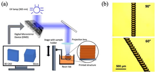
Figure 1.
(a) Schematic diagram of PμSL and resulting surface roughness on a printed part. (b) Microscope images of 3D printed struts in different printing angles (90° and 60°). The polymer used is HDDA and curing time per 80 μm thick layer is 3 s. These side profiles clearly display the surface roughness caused by the layer-wise process.
2. Materials and Methods
2.1. Projection Micro-Stereolithograph (PμSL)
2.1.1. Materials for 3D Printing
In this work, the monomer was 1,6-Hexanediol diacrylate (HDDA), technical grade 80% (Sigma-Aldrich, St. Louis, MO, USA). Phenylbis (2,4,6-trimethylbenzoyl) phosphine oxide (Sigma-Aldrich, St. Louis, MO, USA), also known as its commercial name Irgacure 819, was used as a photoinitiator (PI), and 1-Phenylazo-2-napththol, also called SUDAN-1 (Sigma-Aldrich, St. Louis, MO, USA) was used as a photo-absorber (PA). Ethanol was used to wash away the excess resin after 3D printing.
2.1.2. Projection Micro-Stereolithography (PμSL) Experimental Set-Up
The AM system used in this work is a custom-built PμSL system capable of manufacturing micro-scale features. It consists of a linear stage (Thorlabs), on which the sample holder is attached. A projection lens (Thorlabs) is used to achieve a lateral resolution of 12 μm. A digital micromirror device (DMD) (Texas Instruments, Dallas, TX, USA) is used for generating projection patterns according to cross-sectional digital images of a 3D model. UV LED (365 nm, Hamamatsu, Hamamatsu City, Japan) is used as a UV illumination source. The UV light reflected from the DMD is projected on the surface of the resin inside the vat. Once a layer is formed, the sample holder is lowered by the layer thickness, and the next image is projected to cure a new layer on top of the previous one. This process repeats until all layers are completed. The actual system used in this study is shown in Figure 2. The setup is kept in a printing chamber where environmental factors such as external light and oxygen concentration are controlled.
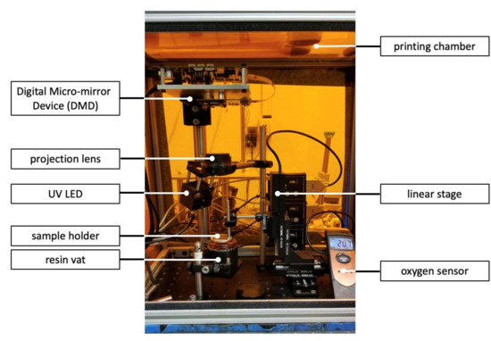
Figure 2.
PμSL experimental setup.
2.2. Computational Model for Photopolymerization Process
2.2.1. Photopolymerization Model
Photopolymerization plays a central role in stereolithography AM processes including PμSL. Photopolymerization occurs in three steps; initiation, propagation, and termination [20]. When UV light is projected on a photocurable resin, free radicals are generated from photoinitiator (initiation). Free radicals readily react with monomer molecules, connecting monomers to form long polymer chains (propagation). Propagation continues until two large chains of polymer cross-link with each other (termination). The liquid resin is converted into a solid when cross-linked polymer network is formed. Environmental conditions are also an important factor that influences the reaction kinetics. Oxygen acts as an inhibitive agent because free radicals react not only with monomer molecules, but also with oxygen molecules when present, forming peroxides. These peroxides do not take part in the polymerization process, thereby inhibiting the overall conversion of liquid resin to solid. This photopolymerization process can be modeled as follows.
Light irradiation intensity (I) which decays as light travels through the resin can be modeled as
where [PI] and [PA] represent photoinitiator and photo absorber concentrations, α is molar absorptivity of photoinitiator, and αa is the molar absorptivity of photo-absorber [21]. The term represents overall absorption coefficient of the resin which follows the Beer–Lambert law [22].
The light intensity of the projected beam is modeled as a convolution of unit light intensity profile which is modeled as a Gaussian function [17]. In Equation (2), w is the beam width of the Gaussian function, I0 is the peak light intensity, and r is the radial position. For n number of activated pixels on DMD, the light intensity distribution on the surface of resin is therefore given by Equation (3).
As descripted in the photopolymerization principle, initiation process consumes photoinitiator molecules which split into free radicals upon irradiation. Accounting for diffusion flux, photoinitiator concentration can be written as [21]
where DPI is diffusivity of photoinitiator, φ is quantum yield of free radicals, and β = 1/3.27 × 105 mol/J is the amount of energy contained in one photon [23].
Upon UV exposure, photoinitiator molecules split to generate free radicals which react with monomers and activate their functional groups. These active monomers react with other monomers and begin a propagation reaction [24], given by
where [M] is monomer concentration, kp is propagation rate constant and [R] is radical concentration. A negative sign indicates that monomer concentration decreases as they are converted into polymer. The radical concentration is given by [25]
where the first term represents radical diffusion with diffusion coefficient Dr, and Rg and Rc account for generation and consumption of free radicals, respectively.
[O] is oxygen concentration, kt is termination rate constant, and ko is oxygen rate constant. The consumption term Rc has two parts: (1) reaction between radicals and (2) reaction with oxygen (oxygen inhibition).
The oxygen concentration is given by [26]
where Do is oxygen diffusion constant.
The conversion ratio C can be determined from monomer concentration [21].
2.2.2. Modeling of Photopolymerization in COMSOL Multiphysics
The photopolymerization model is solved by commercial finite element analysis (FEA) software, COMSOL Multiphysics. We created a 2D axisymmetric domain representing a cross-section of cylindrical volume of resin in the vat of the PμSL system, as shown in Figure 3a.
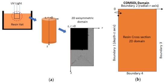
Figure 3.
(a) 2D axisymmetric computational domain representation of UV exposed resin region in the vat. 2D axisymmetric domain consists of two domains that have different mesh sizes due to computational efficiency. (b) Computational domain with boundary conditions.
Here z represents the depth direction along which UV light travels and r is the radial coordinate. The domain is selected in such a way that the light incident on the surface will allow enough area for resin components to diffuse, i.e., the equations for parameter concentrations will be able to converge within the refined mesh area of the domain. The computational domain is divided into two sub regions (higher and lower mesh densities) for computational efficiency. Adaptive time step is used for stability and consistency of the algorithm.
Figure 3b represents the 2D axisymmetric domain and boundary conditions. As the partial differential equations (PDEs) of the photopolymerization process are strongly coupled, COMSOL Multiphysics solves the PDEs iteratively to obtain converged solutions in each time-step. Table 1 lists the initial and boundary conditions.

Table 1.
Initial and boundary conditions.
Following assumptions are made while setting up the simulation.
- Thermal properties are considered to be constant during polymerization reactions. This assumption is made based on the fact that when polymerization on micro scale is limited on a small area, surrounding resin acts a heat sink.
- The rate constants kt and kp are kept constant for simplification of system. Tryson et al. [24] explained more detailed information regarding the change of kt and kp with respect to monomer conversion C.
- Optical effects such as refraction or reflection are not considered.
Table 2 lists constants and their values. When computation is complete, it gives a continuous field of conversion ratio, defined as Equation (10). Interface between cured solid and remaining uncured liquid resin is determined by a cut-off conversion ratio contour, from which curing depth, curing width, and surface profile can be extracted. Detailed method is given in Appendix C and Appendix D.

Table 2.
List of PμSL process parameters. * is from experiments.
2.3. Meta-Heuristic Optimization Technique for Multiple Objectives: Multi-Objective Particle Swarm Optimization (MOPSO)
Improving surface roughness of additively manufactured parts while keeping printing time as small as possible is considered as finding sub-optimal solutions in a parameter search space that satisfies multiple objectives. Because the photopolymerization process involves many parameters and printing variables and a system of PDEs, this problem has highly nonlinear and multivariate response surface. In addition, it is often under various complex constraints. Traditional gradient-based optimization algorithms often fail to find an optimizer of this kind of problems or may be computationally too expensive to calculate derivatives. Recently, various population-based optimization algorithms such as genetic algorithm [30] and ant colony optimization [31] have gained attention because of their derivative-free characteristics and efficiency.
Particle swarm optimization (PSO) is a meta-heuristic optimization algorithm that mimics the social behavior of birds or fish [32]. Each agent evolves and iteratively searches the global optimizer based on its path as well as its neighbors’ paths. Each agent represents a solution of the problem and it will converge to the global optimizer when the iteration ends. PSO has become a useful tool for multiple reasons [33]: (1) since it is not problem specific, it offers a general framework that can be applied to all optimization problems; (2) the algorithm is straightforward and relatively simple to be implemented; (3) it is computationally efficient to find the global optimizer.
Multi-objective particle swarm optimization (MOPSO) is a PSO for multiple objective functions [34]. In MOPSO, the result is a set of different solutions instead of a single global optimizer. It is called a Pareto optimal set. There are three main issues that need to be addressed when PSO extends to MOPSO.
- Selecting a leader for evolving agents
- Retaining the non-dominant solutions in each iteration
- Maintaining diversity of agents during iterations
These issues are addressed in detail when the pseudo-code for MOPSO in Figure 4 is explained.
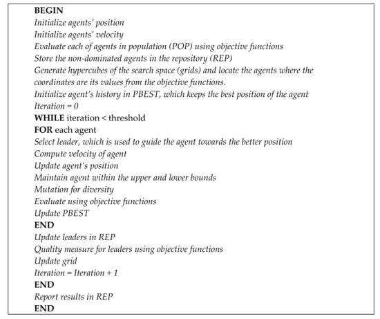
Figure 4.
Pseudo-code for MOPSO.
First, the algorithm initializes agents’ position and velocity. Population (POP) is the memory where all agents’ information in certain iteration is stored. For the initial set, all agents are evaluated based on its randomly distributed positions. Repository (REP) is the external repository where the non-dominated agents in POP are stored. The dominance of each agent is determined by the objective functions. The MOPSO algorithm generates grids that cover all the search space and locate all agents in the grids where the coordinates are its objection function. This controls the density of local agents by determining the local optimizer (leader) that leads neighboring agents. Personal (agent) best position, called PBEST, in the search space keeps the best local optimizer that each agent experiences when it travels through the search space.
When iteration starts, the algorithm updates the velocity of each agent based on Equation (11) [35].
where k is inertia weight, and denote velocity and position of an agent i, at time t, respectively. The underscore indicates that the velocity and position are n-dimensional vectors where n is the number of optimizing parameters. r1 and r2 are random values, . C1 and C2 are constants, called cognitive and social learning factors, respectively. These constants define the amount of attraction toward the agent’s own best experience or that of its neighbors. is the best position that the agent i experienced and is the best position that its neighbor experienced. Each grid has its own in it, so that it helps to explore the entire search space. REP is taken from repository which attracts the agent to the global optimizer in each iteration. By balancing the terms related to C1 and C2, the algorithm enhances the ability to search for the global optimum in the search space. Then, each agent location is updated by Equation (12) [35]
If the position of the agent is located out of the region between the lower and upper bounds that are given by the user, it is forced to be moved inside the valid search space. Then, each agent in POP is evaluated and updated the contents of REP by placing the non-dominated agents within the hypercube. Any dominated agents in REP are removed in this step. When the current status of agent is better than its PBEST, PBEST is updated by the current status. The mutation step is also included to give the diversity of searching ability and increase the opportunity to search the global optimizer. In this study, we used the source code available in the public domain [36] and modify it to match our purpose. The parameters in the algorithm are followed by the basic settings in the source, but the number of agents is reduced to 40 for computational efficiency. The detailed guideline for deciding parameters in PSO and MOPSO algorithm is explained in [33,34].
2.4. MOPSO with COMSOL Multiphysics-MATLAB LiveLink
In order to use the powerful optimization toolboxes and rich built-in libraries in MATLAB, we connected COMSOL Multiphysics with MATLAB via MATLAB LiveLink for COMSOL. Figure 5 shows a schematic description and data flow between MATLAB and COMSOL Multiphysics during our optimization process. The whole process consists of two sub-steps: (1) model calibration and (2) process parameter optimization. First, printing parameters to be calibrated are sampled from the upper and lower bounds of each parameter. Selected printing parameters are sent to the photopolymerization model in COMSOL Multiphysics. COSMOL performs photopolymerization process simulation with given parameters and passes the result (curing depth, in this case) back to MATLAB. This process iteratively finds the calibrated parameters that minimize the deviation between curing depth in experiment and simulation. The calibrated parameters are updated in photopolymerization model in COMSOL Multiphysics.
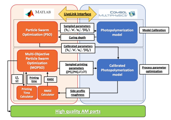
Figure 5.
Flow chart of MATLAB LiveLink interface with COMSOL Multiphysics. Proposed modeling framework consists of two sub-steps: model calibration and process parameter optimization. The flow of data is shown as arrows and labels.
Second, MOPSO samples printing parameters in the parameter search space and passes it to the updated model in COMSOL Multiphysics to obtain surface profile of AM part of given inputs. The surface profile is extracted from photopolymerization simulation and returned to MATLAB. The custom-built MATLAB script calculates root mean squared error (RMSE) value of the given surface profile and uses it as an objective function in the optimization process. The method to calculate RMS for a given surface profile is explained in detail in Appendix D. Another objective function is printing time, which can be calculated by using a custom-built MATLAB script. The detailed method for obtaining printing time is in Section 3.3. This loop continues until it reaches the iteration limit.
3. Results and Discussions
3.1. Model Validation
When a UV light is projected on the surface of a photocurable resin, the liquid resin is converted into solid from the surface to a certain depth. This depth is called curing depth or Cd. The curing depth can be expressed as [20]
where Dp is penetration depth, E is given light energy, and Ec is critical light energy. It is seen that curing depth is proportional to natural logarithm of given light energy. This is known as a working curve for a given resin. Dp and Ec are resin specific characteristic parameters. In this study, we use a set of working curves obtained from experiment to validate our simulation model. The details for obtaining a working curve experimentally is given in Appendix B. In simulation, the conversion ratio C given in Equation (10) is obtained as a continuous field from the initial monomer concentration ([M]0) and the monomer concentration ([M]) remaining after the applied energy dose. The value of C varies between 0 and 1 with 0 being uncured liquid and 1 being fully cured solid. Since a conversion ratio corresponding to the gel point is not readily available from experimental measurement, the conversion ratio value that defines the interface between liquid and cured solid polymer, or ‘cut-off’ conversion ratio, should be chosen to obtain curing depth from simulation. A various range of cut-off conversion ratios have been reported in literature [21], and we used 5% as a conversion cut-off ratio in this study.
In order to validate our computational model, we first experimentally obtained working curves of resins having different PI and PA concentrations. The details regarding sample preparation and post-processing procedure are described in Appendix A. PSO was performed on several simulation constants of ‘ko’, ‘α’, ‘αa’, ‘[O]0’, and ‘C’ to calibrate the computational model. The values of these parameters are reported at a varied range in literature as listed in Table 3. Using RMSE as an objective function, optimization algorithm POS was performed. Table 3 also lists calibrated parameter values after performing PSO. With the calibrated parameters, we performed numerical simulations to obtain working curves for the same resins used in the experiment. Working curves from simulation and experiment are shown in Figure 6 and they show a good agreement. Based on this result, we confirm the validity of our photopolymerization computational model.

Table 3.
List of calibrating parameters.
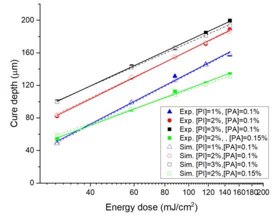
Figure 6.
Comparison of curing depth between experiment and simulation. x-axis represents energy dosage in log scale and y-axis is curing depth in linear scale.
3.2. Effect of Process Parameters on Curing Depth and Width
Since each PμSL process parameter has critical effect on the printing quality, i.e., curing depth and width, evaluation of the effect of each parameter is necessary. Through multiple simulations using the computational model we developed, we studied the impact of each parameter on printing quality of AM parts. Table 4 lists the range of values for each parameter we used for this study. Note that the largest oxygen concentration used in our simulation was 21% as shown in the bold in Table 4 because it is the actual oxygen concentration in the air. Therefore, the corresponding normalized parameter value for this data point is 2.1.

Table 4.
Printing parameter evaluation using normalized value concept.
First, reference curing depth and width were determined from the results produced with the set of parameters in column B. Then, simulations were performed while one parameter was varied with all other parameters being kept constant. Resulting curing depth and width were normalized by the reference value to evaluate the effect of the parameter studied.
Figure 7a shows the effect of the parameters on curing depth. Curing depth increases as (PI) increases because PI increases reactivity of the resin. When (PA) concentration increases, the cure depth reduces because light penetration depth decreases with PA. Cure depth is relatively insensitive to environmental (O). When light intensity and exposure time increase, cure depth increases because light energy is product of light intensity and exposure time. It is observed that (PA) influences cure depth the most, which is also found from results in Figure 6 where Dp and Cd both decrease as (PA) increases.
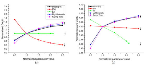
Figure 7.
Effect of printing parameters on (a) curing depth and (b) curing width.
Similar analysis was performed to study the effect of the parameters on curing width. As shown in Figure 7b, it is interesting that environmental oxygen concentration has the highest effect on curing width. As environmental oxygen concentration increases, oxygen inhibition becomes more prominent at the surface of the resin, which results in decrease in curing width. As expected, when (PI), light intensity, and exposure time increase, curing width increases due to increased light energy or reactivity of resin. In contrast to curing depth case, (PA) has least effect on curing width because its role is primarily to control the penetration of light in depth direction.
3.3. Parameter Sensitivity Analysis for Surface Roughness Using Taguchi Orthogonal Array
In PμSL process, a 3D part is built in a layer-by-layer fashion. Since each layer has its own characteristic side profile as a result of photopolymerization reaction, when they are stacked together repeatedly, a distinctive surface roughness arises. This is called the staircase effect. We performed a systematic analysis to study effect of PμSL process parameters on the surface roughness of a 3D printed structure. Since there are many parameters involved, we employed design of experiment (DOE) method proposed by Taguchi to reduce the number of experiments to be performed. This method is known as Taguchi method of orthogonal arrays (OA) [37,38,39]. Figure 8 shows the steps involved in DOE for this study.
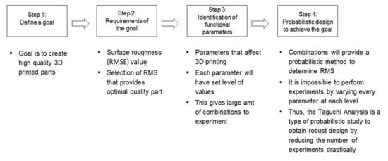
Figure 8.
Steps for developing a robust DOE.
Based on the result obtained in the previous section, we selected (PI), (PA), (O), layer thickness (LT), and curing time (CT) to control surface roughness. We set three levels for each parameter, or ‘factor’. Therefore, the total number of possible combinations of parameters obtainable is 35 = 243. From standard Taguchi OA tables, L27(313) meets the criteria of our analysis where there are five factors with three levels. This dramatically reduces the number of experiment necessary to only 27. Following this, we performed 27 simulations and numerically extracted surface roughness from each simulation. Detailed method to extract surface profile from photopolymerization simulation is described in Appendix D. The factors and their levels, along with surface roughness as response, are shown in Table 5. Surface roughness is measured by RMSE. After obtaining RMSE from each simulation, sensitivity analysis was performed to find the optimal levels for each factor. Signal-to-noise (SN) ratios measure how the response (RMSE value in this study) varies relative to a target value (the expectation set to find optimal factor levels). Since minimum surface roughness would give high quality AM parts, ‘smaller the better’ criterion was chosen to evaluate the factor levels. The formula to calculate SN ratio for ‘smaller the better’ criterion is given by,
where Y is the response of given factor level combination—i.e., RMSE for this case—and n is the number of responses in given factor level combination. Using equation (14), SN ratios for each experiment were obtained and listed in Table 5.

Table 5.
Factor and levels for Taguchi OA.
Based on this result, main effects plots for SN ratios in Figure 9 were generated. Also, a response table (Table 6) was generated, from which the parameters that have the largest effect on the response can be identified. In Figure 9, the average SN ratio of the response is presented by the dotted line. Since the goal here is to find values for each parameter that maximize the SN ratio, the optimal values for each parameter can be determined to achieve the minimum surface roughness. The rank represents which factor affects surface roughness the most. Rank is based on the delta value, which is the difference between the highest and the lowest average SN ratio value for each factor. From the response table, the parameter that affects surface roughness the most is PA concentration, and oxygen concentration has the least impact on surface roughness.
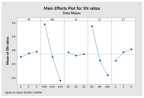
Figure 9.
SN ratio analysis based on RMSE response. The level corresponding to the maximum value of mean of SN ratios is selected for each factor.

Table 6.
Response table for signal-to-noise ratio: smaller the better.
3.4. Optimizing Printing Parameters with MOPSO
Based on the rank from the sensitivity analysis, we selected four highly sensitive parameters that affect surface roughness the most: PI and PA concentrations, layer thickness (LT), curing time (CT). These parameters are used as control parameters in MOPSO algorithm. Since our goal is to determine process parameters to produce high surface quality part as fast as possible, the objectives for MOPSO are RMSE of surface profile of a printed part and printing time. Time required to print a structure (ttotal) is given by
where tlayer is the time required to complete one cycle for a layer and texposure is the curing time that the UV light is exposed on resin surface. tstage is the time required for the linear stage to move sample holder in each process cycle for a layer (measured to be 5 s in experiment). The number of layers is determined by the overall height of structure divided by the layer thickness. In this study, the height that we want to print was set to be 1 mm.
3.4.1. Optimized Printing Parameters for a Vertical Strut
In this section, we apply MOPSO to determine optimal printing parameters that minimizes two objective functions: surface roughness of a printed strut and printing time when the angle of the strut is 90° from the horizontal plane (vertical strut). Table 7 shows the upper and lower bounds of the parameters considered.

Table 7.
List of optimizing parameters.
After performing MOPSO, the graphical representation of Pareto set shown in Figure 10 was generated. x- and y-axis are surface roughness and printing time, respectively. All the agents produce Pareto front, but the shape of Pareto front consists of two major groups, as listed in Table 7. The corresponding objective values are (RMSE = 1.45 μm, printing time = 54.79 s), (RMSE = 1.5 μm, printing time = 48.33 s) for group A and B, respectively. For a vertical strut, higher PI and lower PA improve surface roughness, so that it reduces the surface profile RMSE while giving the small effect on the printing time. In addition, since CT does not change the roughness significantly, it stays at the lower bound to minimize the total printing time, as expected. Table 8 shows the comparison between the several printing times and surface roughness of non-optimized printing examples and optimized examples of Group A and B, shown in the bold in Table 8. The parameter sets for non-optimized printing conditions 1, 2, and 3 are [PI = 65.44 mol/m3, PA = 4.74 mol/m3, LT = 53 μm, CT = 1.00 s, PI = 64.12 mol/m3, PA = 3.04 mol/m3, LT = 80 μm, CT = 2.00 s, PI = 54.09 mol/m3, PA = 2.66 mol/m3, LT = 120 μm, CT = 4.00 s], respectively. When the Group A and the result from non-optimized parameter 1 are compared to each other, it is realized that the proposed optimization framework can reduce the printing time 50% while keeping the surface quality. In addition, the comparison between the Group B and the result from non-optimized parameter 3 shows that the proposed optimization framework reduces 38% of surface roughness when the printing process is at the minimum printing time. Lastly, the result from non-optimized parameters 2 shows the higher printing time and the surface roughness, which often happens when the printing parameters are not optimized. Based on this result, it is clearly seen that the optimized parameters provide better or at least similar surface roughness while significantly reducing printing time.
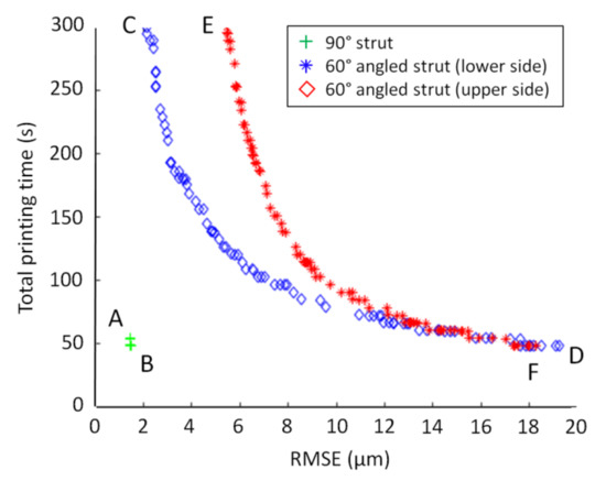
Figure 10.
Pareto optimal sets for a vertical strut (green), optimizing upper side of 60° angled strut (red) in Figure 11, and optimizing lower side of 60° angled strut (blue) in Figure 11. Point C and D are two extremes of optimizing lower side of the 60°angled strut. Point E and F are two extremes of optimizing upper side of the 60° angled strut.

Table 8.
Objectives comparison between optimized and non-optimized printing conditions.
3.4.2. Optimized Printing Parameters for an Angled Strut
To extend our study, we apply the same approach to a 60° angled strut. The objective functions and the considering printing parameters (including the upper and lower bounds) are the same as the vertical strut, but the difference is that surface roughness is different in upper and lower sides. When the angle of the strut is 60° as shown in Figure 11, the result from the upper side of the strut is expected to have no major difference from the vertical strut. However, on the lower side, there exists an additional effect on surface roughness since the light penetration from the upper layer may polymerize resin deeper to the layer below. To visualize this difference, we performed two MOPSO considering surface roughness of the lower and the upper side of a strut and compared the result in Figure 10. The Pareto optimal sets in the figure clearly display the trade-off between surface roughness and printing time; minimizing total printing time increases RMSE, and vice versa. Point C and D are two extremes of optimizing lower side of the 60° angled strut. The optimized parameters of point C and D are (PI = 53.89 mol/m3, PA = 6.10 mol/m3, LT = 20.00 μm, CT = 1.00 s, RMSE = 2.13 μm, printing time = 300.00 s) and (PI = 72.4 mol/m3, PA = 2.03 mol/m3, LT = 120.00 μm, CT = 4.00 s, RMSE = 19.25 μm, printing time = 48.33 s), respectively. It is interesting to see that when the printing time is maximized and RMSE is minimized, PA is the maximum value at the upper bound and LT is minimum value at the lower bound. On the contrary, when the printing time is minimized, LT is maximized and PA is minimized. When the upper side of surface profile is considered, the two extremes E and F are (PI = 60.56 mol/m3, PA = 6.10 mol/m3, LT = 20.00 μm, CT = 1.00 s, RMSE = 5.48 μm, Printing time = 300.00 s) and (PI = 64.30 mol/m3, PA = 3.91 mol/m3, LT = 120.00 μm, CT = 1.00 s, RMSE = 18.28 μm, Printing time = 48.33 s), respectively. The details of all four extremes are displayed in Table 9. This result also supports the high correlation between the RMSE and (PA) and LT as discussed in Section 3.2.
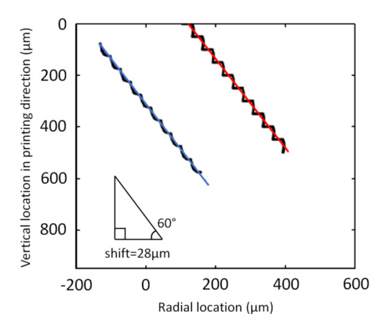
Figure 11.
60° angled strut and its mean profiles for upper (red) and lower (blue) surface profile.

Table 9.
List of optimizing parameters.
The Pareto optimal set clearly visualizes the difference produced by the light penetration. Since the printing time is dominated by LT, the extreme in the printing times between both cases remain the same. However, the surface profile RMSE in Figure 10 shows a clear difference because it is very likely that the light penetrated from the upper layer changes the surface profile. As in the previous section, we compared the optimized examples selected from the Pareto optimal set with the non-optimized examples obtained from the validation set up, as shown in Table 10. The clear difference from the optimization is displayed in the bold in Table 10. The printing parameters for the non-optimized examples are (PI = 54.18 mol/m3, PA = 4.62 mol/m3, LT = 20.00 μm, CT = 1.00 s), (PI = 50.12 mol/m3, PA = 6.08 mol/m3, LT = 28.00 μm, CT = 2.00 s), and (PI = 56.77 mol/m3, PA = 3.13 mol/m3, LT = 120.00 μm, CT = 1.00 s) for example 1, 2, and 3, respectively. The comparison between Point C and the non-optimized point 1 shows the 16% surface quality increase by the proposed optimization framework. In addition, Point D shows 18% surface quality increase even in the fastest printing speed. Therefore, like the previous vertical strut, the comparison between the optimized points and the non-optimized cases, it is clearly seen that the proposed optimization framework significantly increases the efficiency of the printing process.

Table 10.
Objectives comparison between optimized and non-optimized printing conditions.
The clear difference between the Pareto sets of the upper and lower side profiles, shown in Figure 10, is expected for other angled struts. The degree of effect from the light penetration from the upper layer on the surface roughness of the lower layer will be different because the area affected by the light penetration is different, depending on the printing angle. The optimization method presented here can be easily applied to other 3D printed geometries that may have different side slopes.
It is very important to know the configuration of the Pareto optimal set between these two extremes. Different points on this set allow us to have different printing set-up and corresponding printing time and RMSE, but its printing time and roughness are limited by these two extremes. Therefore, this Pareto optimal set can be a guideline to make better printing conditions depending on the need. The usability of MOPSO is even more obvious when the result from MOPSO is compared with the non-optimized printing case. The approach described in this section can be extended to other printing angles or complex surface profile. It can also be possible to use different objective functions, such as the mechanical strength, total mass, or other properties of AM parts. Based on these results, we conclude that the MOPSO for PµSL helps to optimize the cost functions of interest. In addition, it offers a design guideline for the performance measure for AM parts.
4. Conclusions
We present a systematic approach that provides the optimal printing process parameters for high quality AM parts using a computational model and the particle swarm optimization algorithm. A computational model representing the photopolymerization kinetics involved in PµSL process was implemented and process constants were carefully calibrated by using experimental data obtained from a custom-built PµSL system. Taguchi’s Orthogonal Array (OA) method was used to select the parameters that affect the surface quality of AM parts significantly. Four process parameters (PI and PA concentrations, layer thickness, and curing time) selected from Taguchi’s OA were used as controlling parameters for optimization algorithm. A meta-heuristic population-based optimization algorithm, particle swarm algorithm for multiple objectives, called multi-objective particle swarm optimization (MOPSO), was used to determine optimal printing process parameters with given geometry of AM parts. Two struts with different printing angles (vertical and 60°) were considered and the optimized printing process parameters were determined for each case. The Pareto optimal set in each printing angle was obtained so that it can be used as a guideline when the printing process parameters need to be set. The result showed that the proposed optimization framework reduces 50% of printing time while keeping the surface quality equal for the vertical strut, and increases 18% of surface quality of the angled strut even in the fastest printing speed, compared to the samples produced by using non-optimized parameters. This framework consisting of the computational model for photopolymerization, process parameter selection by Taguchi’s method, and MOPSO for optimization printing process parameters resulted in significant improvement in the quality of AM parts while keeping the printing time minimum. By changing the objective functions of MOPSO, presented approach can also be used for optimizing various quality measures, such as minimizing printing cost and maximizing mechanical strength. Our proposed optimization technique can be easily applied to other photocurable polymers by incorporating material-specific photocuring kinetics parameters for a given polymer in the photopolymerization process modeling. In addition, increasing dimensionality of search space in MOPSO is straightforward without modification of the algorithm, so multiple printing parameters as well as external inputs can be easily increased by adding an additional dimension in the search space. We believe that the process optimization method presented in this study helps to achieve high-quality 3D printed structures and that it can be easily extended to other AM techniques where trial-and-error approaches are used to determine process parameters.
Author Contributions
Conceptualization, H.L.; Data curation, N.K., I.M.B., and D.H.; Formal analysis, N.K., I.M.B., D.H., and H.L.; Funding acquisition, H.L.; Investigation, N.K., I.M.B., and H.L.; Methodology, N.K., I.M.B., D.H., C.Y., and H.L.; Project administration, H.L.; Resources, C.Y. and H.L.; Software, N.K. and I.M.B.; Supervision, H.L.; Validation, N.K. and I.M.B.; Visualization, N.K. and I.M.B.; Writing—original draft, N.K. and I.M.B.; Writing—review and editing, N.K., I.M.B., and H.L.
Funding
This research was funded by Rutgers University through the School of Engineering and the Department of Mechanical and Aerospace Engineering.
Conflicts of Interest
The authors declare no conflict of interest.
Appendix A. Sample Preparation for Curing Depth Study
The cure depth study was performed by printing the bridge structures shown in Figure A1. A single layer in a rectangular shape supported at its both ends was printed. Since there is no supporting layer underneath, thickness of each bridge is the curing depth of the layer. A single structure was designed in which five bridges could be printed for each different energy dose. Each structure has two columns of bridges and each structure was printed twice, thus giving four bridge samples for each set of parameters. These protruding notches were added at the center of the bridge supports to help to bring the structure to a focal plane of a microscope during thickness measurement. After each structure was printed, it was placed in ethanol for 3 s and then let dry in the air. The measurements were done as described in Appendix B. Table A1 lists the printing parameters varied.

Figure A1.
Bridge structure illustration for cure depth measurement.

Table A1.
Printing parameters for HDDA.
Table A1.
Printing parameters for HDDA.
| Concentration Level | Photoinitiator (PI) | Photo-Absorber (PA) | Environmental O2 (O) | |||
|---|---|---|---|---|---|---|
| (mol/m3) | % | (mol/m3) | % | (mol/m3) | % | |
| Low | 24.14 | 1 | 4.06 | 0.1 | 8.69 | 21 |
| Medium | 48.27 | 2 | 6.1 | 0.15 | - | - |
| High | 72.4 | 3 | - | - | - | - |
Appendix B. Curing Depth Measurement in Experiment
A printed sample was first placed under an optical microscope with a digital camera attached. A 5× lens was selected for measurement. The stage of the microscope was adjusted until the bridge layers came into focus. Digital images of the bridges were captured. The thickness of each bridge was measured using image analysis software, ImageJ. Each cure depth was measured at the center of the bridge as shown in Figure A2. The value obtained from this measurement was in pixels and the pixel to microns conversion was done based on the image size and conversion factor which was obtained from calibration.
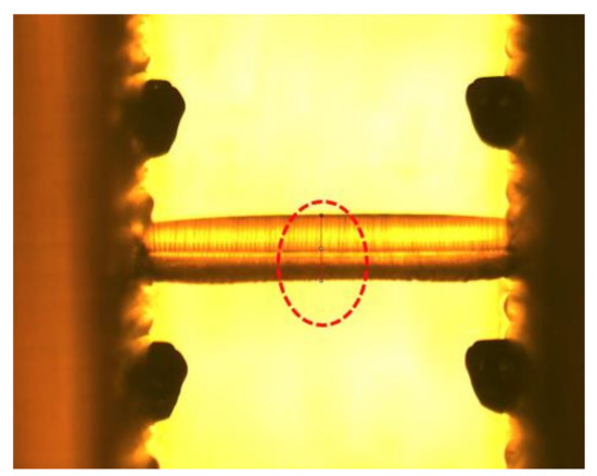
Figure A2.
Use of ImageJ line tool to measure curing depth. The optical lens is focused on the notches to find optimal depth. Pixel length of line drawn at the center of the layer. Conversion is done to microns based on conversion factor.
Appendix C. Constructing Cured Profile in Simulation
Figure A3a shows a conversion ratio contour plot generated from COMSOL Multiphysics simulation. A contour line corresponding to 5% cut-off conversion ratio was extracted and mirrored to construct a full cross-section as shown in Figure A3b. Light attenuation along z-direction results in a trapezoidal shaped curing pattern. This plot was used obtain curing width and curing depth of the layer.
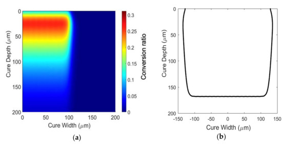
Figure A3.
Conversion contour layer profile extraction: (a) Conversion contour for layer profile; (b) Extracted shape of the cured profile based on the 4% (0.04) cutoff conversion ratio contour.
Appendix D. Calculating Surface Roughness as RMSE
The RMSE was used to quantify surface roughness of AM parts. Once a layer thickness to be used in PµSL process is specified, the bottom portion of the cross-section in Figure A3b below the layer thickness was trimmed away, leaving a cross-section profile of each layer. The layer-wise PµSL process was emulated by stacking this cross-section. A 2D representation of vertically stacked layers is shown in Figure A4. The mean line of the surface profile was first obtained, from which profile deviations were calculated. Subsequently, RMSE of the surface profile was calculated. A similar approach was used for angled struts.
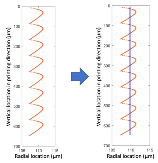
Figure A4.
Mean line (blue) on top of surface profile extracted from the simulation data.
Appendix E. Table for Acronyms

Table A2.
Table for acronyms.
Table A2.
Table for acronyms.
| Acronym | Definition |
|---|---|
| AM | Additive Manufacturing |
| PμSL | Projection Micro Stereolithograpy |
| CAD | Computer-Aided Design |
| HDDA | Hexanediol Diacrylate |
| PI | Photoinitiator |
| PA | Photo-absorber |
| DMD | Digital Micromirror Device |
| PDE | Partial Differential Equation |
| PSO | Particle Swarm Optimization |
| MOPSO | Multi-Objective Particle Swarm Optimization |
| RMSE | Root Mean Squared Error |
| DOA | Design of Experiment |
| OA | Orthogonal Array |
| LT | Layer Thickness |
| CT | Curing Time |
| DOF | Degree of Freedom |
References
- Melchels, F.P.; Feijen, J.; Grijpma, D.W. A review on stereolithography and its applications in biomedical engineering. Biomaterials 2010, 31, 6121–6130. [Google Scholar] [CrossRef]
- Alapan, Y.; Hasan, M.N.; Shen, R.; Gurkan, U.A. Three-dimensional printing based hybrid manufacturing of microfluidic devices. J. Nanotechnol. Eng. Med. 2015, 6, 021007. [Google Scholar] [CrossRef] [PubMed]
- Vaezi, M.; Seitz, H.; Yang, S. A review on 3D micro-additive manufacturing technologies. Int. J. Adv. Manuf. Technol. 2013, 67, 1721–1754. [Google Scholar] [CrossRef]
- Frenzel, T.; Findeisen, C.; Kadic, M.; Gumbsch, P.; Wegener, M. Tailored Buckling Microlattices as Reusable Light-Weight Shock Absorbers. Adv. Mater. 2016, 28, 5865–5870. [Google Scholar] [CrossRef] [PubMed]
- Maloney, K.J.; Fink, K.D.; Schaedler, T.A.; Kolodziejska, J.A.; Jacobsen, A.J.; Roper, C.S. Multifunctional heat exchangers derived from three-dimensional micro-lattice structures. Int. J. Heat Mass Transf. 2012, 55, 2486–2493. [Google Scholar] [CrossRef]
- Warnke, P.H.; Douglas, T.; Wollny, P.; Sherry, E.; Steiner, M.; Galonska, S.; Becker, S.T.; Springer, I.N.; Wiltfang, J.; Sivananthan, S. Rapid prototyping: porous titanium alloy scaffolds produced by selective laser melting for bone tissue engineering. Tissue Eng. Part C: Methods 2008, 15, 115–124. [Google Scholar] [CrossRef] [PubMed]
- Han, D.; Farino, C.; Yang, C.; Scott, T.; Browe, D.; Choi, W.; Freeman, J.W.; Lee, H. Soft Robotic Manipulation and Locomotion with a 3D Printed Electroactive Hydrogel. ACS Appl. Mater. Interfaces 2018, 10, 17512–17518. [Google Scholar] [CrossRef] [PubMed]
- Hornick, J. 3D printing in Healthcare. J. 3D Printing Med. 2017, 1, 13–17. [Google Scholar] [CrossRef]
- Campbell, T.; Williams, C.; Ivanova, O.; Garrett, B. Could 3D Printing Change the World. Technologies, Potential, and Implications of Additive Manufacturing; Atlantic Council: Washington, DC, USA, 2011. [Google Scholar]
- Meza, L.R.; Greer, J.R. Mechanical characterization of hollow ceramic nanolattices. J. Mater. Sci. 2014, 49, 2496–2508. [Google Scholar] [CrossRef]
- Ahn, D.; Kim, H.; Lee, S. Surface roughness prediction using measured data and interpolation in layered manufacturing. J. Mater. Process. Technol. 2009, 209, 664–671. [Google Scholar] [CrossRef]
- Sager, B.; Rosen, D.W. Use of parameter estimation for stereolithography surface finish improvement. Rapid Prototyp. J. 2008, 14, 213–220. [Google Scholar] [CrossRef]
- Hasan, R. Progressive Collapse of Titanium Alloy Micro-Lattice Structures Manufactured Using Selective Laser Melting. Ph.D. Thesis, University of Liverpool, Liverpool, UK, 2013. [Google Scholar]
- Quintana, R.; Choi, J.-W.; Puebla, K.; Wicker, R. Effects of build orientation on tensile strength for stereolithography-manufactured ASTM D-638 type I specimens. Int. J. Adv. Manuf. Technol. 2010, 46, 201–215. [Google Scholar] [CrossRef]
- Ancau, M.; Caizar, C. The optimization of surface quality in rapid prototyping. In Proceedings of the WSEAS International Conference on Engineering Mechanics, Structures, Engineering Geology (EMESEG ‘08), Crete Island, Greece, 22–24 July 2008. [Google Scholar]
- Chockalingam, K.; Jawahar, N.; Chandrasekhar, U. Influence of layer thickness on mechanical properties in stereolithography. Rapid Prototyp. J. 2006, 12, 106–113. [Google Scholar] [CrossRef]
- Sun, C.; Fang, N.; Wu, D.; Zhang, X. Projection micro-stereolithography using digital micro-mirror dynamic mask. Sens. Actuators A: Phys. 2005, 121, 113–120. [Google Scholar] [CrossRef]
- Decker, C.; Jenkins, A.D. Kinetic approach of oxygen inhibition in ultraviolet-and laser-induced polymerizations. Macromolecules 1985, 18, 1241–1244. [Google Scholar] [CrossRef]
- Jariwala, A.S.; Ding, F.; Boddapati, A.; Breedveld, V.; Grover, M.A.; Henderson, C.L.; Rosen, D.W. Modeling effects of oxygen inhibition in mask-based stereolithography. Rapid Prototyp. J. 2011, 17, 168–175. [Google Scholar] [CrossRef]
- Odian, G. Principles of Polymerization; John Wiley & Sons: Hoboken, NJ, USA, 2004. [Google Scholar]
- Fang, N.; Sun, C.; Zhang, X. Diffusion-limited photopolymerization in scanning micro-stereolithography. Appl. Phys. A 2004, 79, 1839–1842. [Google Scholar] [CrossRef]
- Ingle, J.D., Jr.; Crouch, S.R. Spectrochemical Analysis; Prentice-Hall: Inglewood Cliffs, NJ, USA, 1988. [Google Scholar]
- Rohatgi-Mukherjee, K. Fundamentals of Photochemistry; Wiley Eastern Ltd.: New Delhi, India, 1978. [Google Scholar]
- Tryson, G.; Shultz, A. A calorimetric study of acrylate photopolymerization. J. Polym. Sci.: Polym. Phys. Ed. 1979, 17, 2059–2075. [Google Scholar] [CrossRef]
- Zhao, Z.; Mu, X.; Wu, J.; Qi, H.J.; Fang, D. Effects of oxygen on interfacial strength of incremental forming of materials by photopolymerization. Extreme Mech. Lett. 2016, 9, 108–118. [Google Scholar] [CrossRef]
- Dendukuri, D.; Panda, P.; Haghgooie, R.; Kim, J.M.; Hatton, T.A.; Doyle, P.S. Modeling of oxygen-inhibited free radical photopolymerization in a PDMS microfluidic device. Macromolecules 2008, 41, 8547–8556. [Google Scholar] [CrossRef]
- Florio, J.J.; Miller, D.J. Handbook of Coating Additives; CRC Press: Boca Raton, FL, USA, 2004. [Google Scholar]
- Brandrup, J.; Immergut, E.H.; Grulke, E.A.; Abe, A.; Bloch, D.R. Polymer Handbook; Wiley: New York, NY, USA, 1989; Volume 7. [Google Scholar]
- Flach, L.; Chartoff, R.P. A process model for nonisothermal photopolymerization with a laser light source. I: Basic model development. Polym. Eng. Sci. 1995, 35, 483–492. [Google Scholar]
- Deb, K.; Pratap, A.; Agarwal, S.; Meyarivan, T. A fast and elitist multiobjective genetic algorithm: NSGA-II. IEEE Trans. Evol. Comput. 2002, 6, 182–197. [Google Scholar] [CrossRef]
- Dorigo, M.; Birattari, M. Ant colony optimization. In Encyclopedia of Machine Learning; Springer: Berlin, Germany, 2011; pp. 36–39. [Google Scholar]
- Eberhart, R.; Kennedy, J. A new optimizer using particle swarm theory. In Proceedings of the Sixth International Symposium on Micro Machine and Human Science, MHS’95, Nagoya, Japan, 4–6 October 1995; pp. 39–43. [Google Scholar]
- Reyes-Sierra, M.; Coello, C.C. Multi-objective particle swarm optimizers: A survey of the state-of-the-art. Int. J. Comput. Intell. Res. 2006, 2, 287–308. [Google Scholar]
- Coello, C.A.C.; Pulido, G.T.; Lechuga, M.S. Handling multiple objectives with particle swarm optimization. IEEE Trans. Evol. Comput. 2004, 8, 256–279. [Google Scholar] [CrossRef]
- Kennedy, J. Particle swarm optimization. In Encyclopedia of Machine Learning; Springer: Berlin, Germany, 2011; pp. 760–766. [Google Scholar]
- Yarpiz. Multi-Objective Particle Swarm Optimization (MOPSO). Available online: www.yarpiz.com (accessed on 3 November 2018).
- Taguchi, G. Introduction to Quality Engineering: Designing Quality into Products and Processes; Asian Productivity Organization: Tokyo, Japan, 1986. [Google Scholar]
- Ross, P.J. Taguchi Techniques for Quality Engineering: Loss Function, Orthogonal Experiments, Parameter and Tolerance Design; McGraw-Hill: New York, NY, USA, 1988. [Google Scholar]
- Peace, G.S. Taguchi Methods: A Hands-On Approach; Addison-Wesley: Reading, MA, USA, 1993. [Google Scholar]
© 2019 by the authors. Licensee MDPI, Basel, Switzerland. This article is an open access article distributed under the terms and conditions of the Creative Commons Attribution (CC BY) license (http://creativecommons.org/licenses/by/4.0/).